Abstract
The coconut is a perennial, evergreen tree in the palm family that belongs to the monocotyledonous group. The coconut plant holds significant economic value due to the diverse functions served by each of its components. Any ailment that impacts the productivity of the coconut plantation will ultimately have repercussions on the associated industries and the sustenance of the families reliant on the coconut economy. Deep learning has the potential to significantly alter the landscape of plant disease detection. Convolutional neural networks are trained using extensive datasets that include annotated images of plant diseases. This training enables the models to develop high-level proficiency in identifying complex patterns and extracting disease-specific features with exceptional accuracy. To address the need for a large dataset for training, an Enhanced Visual Geometry Group (EVGG16) model utilizing transfer learning was developed for detecting disease infections in coconut trees. The EVGG16 model achieves effective training with a limited quantity of data, utilizing the weight parameters of the convolution layer and pooling layer from the pre-training model to perform transfer Visual Geometry Group (VGG16) network model. Through hyperparameter tuning and optimized training batch configurations, we achieved enhanced recognition accuracy, facilitating the development of more robust and stable predictive models. Experimental results demonstrate that the EVGG16 model achieved a 97.70% accuracy rate, highlighting its strong performance and suitability for practical applications in disease detection for plantations.
1. Introduction
Precise diagnosis and categorization of plant diseases are crucial for the advancement of precision agriculture and organic farming. For plant disease identification, relying on human observation of disease symptoms on plant leaves and diagnosing plant diseases based on experience is highly subjective, inefficient, and prone to misjudgment. Biotechnological methods, on the other hand, are complex to operate, require specialized knowledge and skills, and are time-consuming, making them unsuitable for rapid monitoring. These approaches, clearly, cannot meet the development needs of modern agricultural informatization and intelligence. Although manual observation and biotechnological methods have been employed to detect diseases, image-based methods have become popular due to their non-intrusive nature and relative ease of capturing plant images. Conventional methods may encounter problems in extracting meaningful features or accurate segmentation in the presence of complex backgrounds, lighting conditions, or shadows in the images. With the advent and advances of deep learning, image-based approaches using deep learning have been widely used in agricultural plant disease detection research [1]. These approaches have surmounted the limitations of traditional methods and yielded superior outcomes.
The integration of deep learning into plant disease detection brings multiple benefits. First and foremost, it relieves the burden of tedious manual feature selection and preprocessing that traditionally characterize image recognition methods. Deep learning models autonomously learn to extract meaningful and relevant features, eliminating the need for human intervention [2].
In addition, deep learning enables the development of more robust and adaptive plant disease detection systems. These models can be fine-tuned and continuously updated with new data, enabling continuous improvement in their performance and accuracy, a critical feature in the dynamic agricultural field where disease prevalence can vary with seasons and geographic regions [3]. In summary, the integration of deep learning into plant disease detection opens new vistas for research and development in precision agriculture. Its potential to revolutionize disease detection and management promises to make a significant contribution to sustainable progress and increase efficiency in crop production.
The introduction of advanced image processors and the widespread use of Convolutional Neural Networks (CNNs) in deep learning have established a strong hardware foundation and a wealth of technological advancements to facilitate the progress of artificial intelligence [4]. Deep learning models have a remarkable capacity to independently extract informative characteristics by progressing through layers, starting from raw pixel-level input and advancing toward abstract semantic notions. Their intrinsic advantage allows them to extract global information from photos, offering innovative methods for detecting plant diseases [5].
Transfer learning addresses the issue of requiring a large amount of data for training deep learning models [6]. Transfer learning in deep learning involves utilizing pre-trained model parameters in new models to enhance the training process, transfer annotated data or knowledge structures from related domains, and enhance the learning performance in target recognition domains. Not only does it significantly minimize the model’s training cycle, but it also decreases the training loss rate and enhances testing accuracy [7].
Advanced methods have been applied to detect diseases in oil palm plantations. However, not much has been done for coconut palm plantations, even though both plants are from the same palm family. Piyush Singh et al. [8] trained the custom-designed deep 2D Convolutional Neural Network (CNN) to predict diseases and pest infections. Additionally, the state-of-the-art Keras pre-trained CNN models VGG16, VGG19, and InceptionV3 were fine-tuned using transfer learning to accurately classify images as either infected or healthy. Furthermore, Inception-ResNetV2 and MobileNet obtained a classification accuracy of 81.48% and 82.10%, respectively. Krishnamoorthy et al. [2] integrated the pre-trained deep convolutional neural network Inception-ResNetv2 with transfer learning methods for rice leaf disease recognition and optimized the model’s parameters for the recognition task, resulting in a recognition accuracy of 95.67%. Yue et al. [3] improved the VGG network by integrating high-order residual and parameter-shared feedback sub-networks. The high-order residual sub-network provided higher accuracy in disease recognition by capturing the apparent features of the crop disease.
The application of deep learning techniques to plant disease detection has indeed led to remarkable success in terms of classification accuracy. However, certain challenges and complexities remain, such as the inadequacy of the data samples, the suboptimal robustness of the models, the large variability of disease symptoms, and the complicated backgrounds of the images. Therefore, when dealing specifically with coconut diseases, it is imperative to conduct a thorough comparative analysis of existing models and refine them to determine the most appropriate model. The focus of this research is enhancing the existing VGG16 model by adding Batch Normalization (BN) and Global Average Pooling (GAP) layers. In addition, the proposed enhanced VGG16 model utilizes transfer learning, adjusting hyperparameters and training batches to achieve more accurate recognition and obtain a more stable and accurate prediction model. The model proposed in this study aims to help farmers identify pests and diseases in coconut trees at an early stage, thereby ensuring the smooth production of coconuts.
2. Methodology
This section presents the phases for developing the proposed model.
2.1. Proposed Model
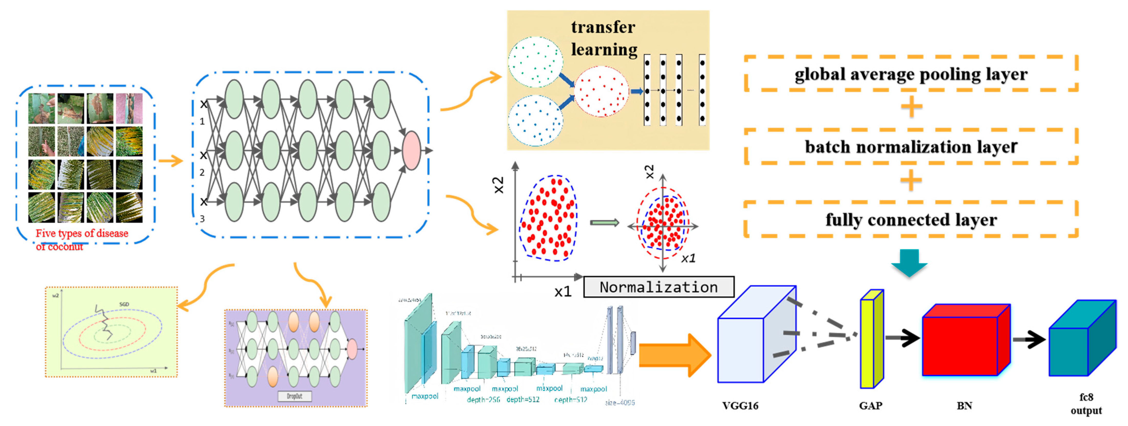
Figure 1 illustrates the proposed EVGG16 for transfer learning. The EVGG16 model retains pre-trained convolutional layers and replaces the three fully connected layers with GAP layers, BN layers, and fully connected layers. For hyperparameters optimization, the Stochastic Gradient Descent (SGD) algorithm is used to process a training sample in each iteration and then update the parameters, so that the training speed is fast. In addition, SGD possesses an exceptional ability to converge swiftly to a local optimal solution. Therefore, the model adopts SGD, specifies the initial value and decay rate of the learning rate, and then induces the exponential decay of the rate.

Figure 1.
Components of the EVGG16 model for disease infection classification in coconut trees.
2.2. Data
The dataset for this research was obtained from Kaggle. It is a publicly accessible dataset and comprises images of five distinct coconut leaf diseases, all in JPEG format. Detailed dataset characteristics are provided in Table 1, with sample images displayed in Figure 2. The dataset includes images representing five specific coconut leaf diseases: leaflets, caterpillars, yellowing, drying, and flaccidity. For effective model training and evaluation, the dataset was divided into a training set (80%) and a testing set (20%). The dataset was primarily acquired in the field. The coconut tree in the picture is from India. The number of images for five specific coconut leaf diseases is relatively balanced. To further ensure data balance, preprocessing methods such as image scaling, rotation, and cropping should be implemented in the testing and training datasets.

Table 1.
Types of coconut leaf diseases in the dataset.
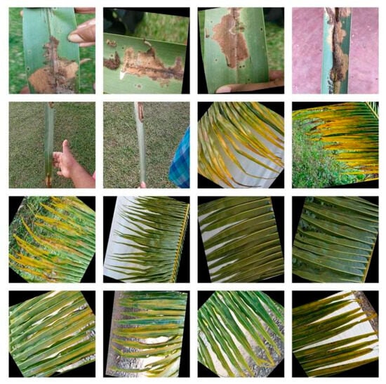
Figure 2.
Examples of coconut tree disease.
2.3. Convolutional Neural Network Architecture
A CNN is a type of deep neural network that was initially developed to analyze images. Recent discoveries have revealed that CNNs possess exceptional proficiency in analyzing sequence data, including natural language processing. A CNN comprises two fundamental operations: convolution and pooling. By employing numerous filters in the convolution operation, we may extract distinctive characteristics from the input signals while preserving their respective spatial information [8].
2.3.1. Input Layer
Convolutional Neural Networks (CNNs) are designed to process high-dimensional data efficiently. Lower-dimensional convolutions are applied to low-dimensional arrays, while higher-dimensional convolutions handle more complex, high-dimensional data. For example, 1D convolutions are commonly used for sequential data like speech signals, whereas 2D and 3D convolutions are primarily used for processing images and videos, capturing both spatial and temporal patterns across dimensions. Black-and-white images are represented as two-dimensional arrays, with pixel values on a plane, while color images incorporate RGB channels, forming a three-dimensional array for input processing. This research specifically utilizes color images, leveraging the additional dimensionality of RGB channels for enhanced feature extraction and analysis.
2.3.2. Convolution Layer
The convolution layer serves as the central component of the convolution neural network, with its primary purpose being the extraction of features from the input image. Multiple convolution kernels are contained within the convolution layer. The feature map of this layer is obtained by integrating the convolution kernel and the output of the image from the previous layer. In the convolution layer, the output consists of numerous feature maps. Three parameters comprise the convolution kernel: the size of the kernel, the stride, and the padding. In a convolution neural network, the range of the local perceptual domain is determined by the convolution kernel size.
2.3.3. Pooling Layer
The pooling layer generally abstracts and reduces the dimension of the input feature map between consecutive convolution layers by taking part of the continuous area of the image as the pooled area and then letting the sliding window matrix of the preset pooling function translate within the area. Finally, it replaces the feature map of the adjacent area with the results of a single point in the matrix. The pooled size and step size control the sliding window size and translation rules.
2.3.4. Activation Layer
In the neural network, every neuron node receives the output value of the preceding layer as its input value. It then proceeds to transmit the input value to the subsequent layer. The input attribute value is transmitted directly from the neuron node in the input layer to the subsequent layer, which may be the hidden or output layers. The activation function denotes the functional relationship between the input of the lower node and the output of the upper node in a multi-layer neural network. After convolution operations, the image uses activation functions [9,10] to assist in expressing complex features. The activation functions introduce nonlinear factors to the neurons of the artificial neural network. Therefore, neural networks can infinitely approximate arbitrary nonlinear functions, effectively improving the network’s feature extraction and expression capabilities.
2.3.5. Output Layer
Consecutively, the output layer concludes the convolutional neural network. It operates on a principle similar to that of the conventional feedforward neural network. The output layer generates classification labels by utilizing logic functions that are referenced from the final full connection layer. The sigmoid function is frequently employed to transform the score result into a classification probability for binary classification problems. In general, image recognition is a multi-classification problem for which a SoftMax normalized exponential function is typically employed.
2.4. VGG16 and Transfer Learning
2.4.1. VGG16
VGGNet is predicated on the repetitive stacking of smaller convolutional kernels to increase the network’s depth. Two fundamental varieties exist: VGGNet-16 and VGGNet-19. In consequence, convolutional neural networks have initiated a vertical deepening development with the appearance of deep network models including GoogleNet and ResNet. As illustrated in Figure 3, the VGG16 comprises thirteen convolutional layers, three completely connected layers, and a SoftMax output layer. For each activation unit in the concealed layers, the ReLU function is utilized. To increase the number of channels, more intricate and expressive features should be extracted and a convolution kernel with a capacity of 3 × 3 should be implemented. Between layers, sampling to capture finer information employs the maximum pooling approach with a 2 × 2 size configuration. As the number of convolution layers increases, so does the number of convolution kernels; the convolution layer depth is as follows: 64 → 128 → 256 → 512 → 512.
2.4.2. Transfer Learning
A substantial annotated image dataset is generally necessary for CNNs to attain a notable level of predictive accuracy. However, such data are difficult to obtain and expensive to label in numerous regions. Given the difficulties, numerous prior investigations have implemented the notion of transfer learning to address cross-domain image classification issues; this approach has proven to be highly advantageous [11,12,13,14]. Transfer learning reapplies the trained model to a different classification task, this time for image recognition, and reclassifies the previously learned features as characteristics of new data. The process consists of the following steps: initialize the basic model and load the pre-trained weights into it; freeze all the layers comprising the basic layer; construct a new fully connected layer or classifier layer atop the output of one or more basic layers; and, finally, train the newly constructed model using the new dataset. In their study, Yang et al. [15] applied the migrated pre-training model of Inception V3 in GoogleNet to a dataset containing ten different types of fruits. The accuracy achieved for both training and testing was greater than 94%. Feature transfer is a prevalent approach in transfer learning, wherein the final layer of the pre-trained network is eliminated and its previous activation values, which can be conceptualized as feature vectors, are transmitted to classifiers for training [16,17,18].
2.5. Improved CNNs Based on VGG16
This model enhances the VGG16 model by substituting the three fully connected layers in the original model with a fully connected layer, a batch normalization layer, and a global average pooling layer. While a batch normalization layer can accelerate convergence, a global average pooling layer can reduce the number of parameters. The ImageNet-trained VGG16 should be employed for transfer learning as shown in Figure 3.
2.5.1. Batch Normalization (BN)
While neural networks exhibit greater sensitivity to data near zero, as the number of network layers increases, the characteristic data begin to diverge from the mean value of zero. Standardization can conform the data to a mean value of zero and a standard deviation distribution of one, thereby restoring the offset characteristic data to an approximate value of zero. Batch normalization transforms the input of every layer in the neural network so that it conforms to the standard normal distribution, which has a mean of zero and a standard deviation of one. Its objective is to address the gradient disappearance issue in neural networks [19].
2.5.2. Global Average Pooling Layer (GAP)
Widely employed CNN network models at this juncture employ the complete connection layer of each algorithm model to classify and output the processed data after the execution of corresponding operations, including convolution feature extraction and aggregation of the initial input image. When the original input image pixels are large or the number of full connection layers in the network model is excessive, a considerable number of parameters is appended between the full connection layers following convolution, pooling, and the final full connection output. This results in the CNN network model calculating a substantial number of parameters during both training and prediction, ultimately diminishing the model’s efficiency. A significant increase in the quantity of parameters during the training process also results in the development of overfitting. The introduction of global average pooling significantly mitigates the issues. A one-dimensional vectorized average aggregated window of the same size as the graph is connected to the SoftMax classifier to generate a classification output. Global average pooling also serves the crucial function of regularizing the structure of the entire convolutional neural network, thereby mitigating the overfitting phenomenon that can arise from an excessive number of full connection layer parameters [20].
2.5.3. Optimizer
The optimization algorithm updates the parameters of the filter in the process of backpropagation to reduce the error. Due to the parameter values of the randomly initialized filter, losses will occur in the forward propagation phase. It needs to be adjusted to reduce losses. The optimization algorithms often used in convolutional neural networks include the Stochastic Gradient Descent (SGD) and the Adaptive Moment Estimation (Adam). The selection of the optimization function needs to be based on specific classification tasks. Different algorithms have different optimization effects. The SGD algorithm processes a training sample in each iteration and then updates the parameters; therefore, the training speed is fast. One potential drawback of the SGD algorithm is that it may be challenging to initialize an appropriate learning rate during the training phase of the network model. Additionally, SGD can readily converge to the local optimal solution. The Adam algorithm modifies the learning rate of each parameter dynamically by employing gradient moment estimations of the first and second orders [21]. Following offset correction, the learning rate varies within a specific range, resulting in increased parameter stability. It integrates the benefits of adaptive gradient and of the root mean square. The adaptive gradient excels at handling sparse gradients, while the root mean square excels at handling non-stationary targets. It is well-suited for large datasets and high-dimensional spaces. Nevertheless, Adam has the potential to disrupt the learning rate during the final stages of training, a phenomenon which could prevent the model from converging. We implement gradient descent, specify the initial value and decay rate of the learning rate, and subsequently induce an exponential decay of the rate [22].
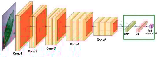
Figure 3.
CNN based on VGG16 [23].
Figure 3.
CNN based on VGG16 [23].

2.5.4. ReLU
ReLU represents a significant advancement in neural network research over the past few years. To begin with, backpropagation operations effectively address the issue of gradient disappearance by always setting the gradient to 1 for inputs greater than 0. Conversely, inputs less than 0 result in a constant output of zero, thereby enhancing the network’s generalization capability and sparsity. Furthermore, it is worth noting that ReLU, being a linear operation, substantially diminishes the computational complexity of the system. In comparison to the sigmoid and tanh functions, this reduction is of an order of magnitude. Consequently, the network convergence speed is greatly enhanced, and the training time expenditure for deep neural networks is diminished.
Compared to traditional sigmoid and tanh activation functions, the implementation of ReLU only involves threshold judgment and does not involve any exponential operations, making it very computationally efficient. In the training process of neural networks, computing resources are extremely valuable, and the simplicity of ReLU can significantly reduce training time and computational costs. In practical applications, neural networks using ReLU activation functions tend to converge faster than networks using sigmoid or tanh functions. This is because the gradient of ReLU in the positive interval is always 1, which is beneficial for the gradient descent method to move quickly in the parameter space without being affected by the disappearance of gradients, thereby accelerating the learning process. The ReLU function directly outputs 0 when the input is less than 0, something which can cause only a portion of the hidden neurons in the network to be activated, resulting in a sparse activation phenomenon. Sparsity can improve the expressive power of a network and reduce the risk of overfitting, as the model only needs to adjust those neurons that contribute to the output, making the model more robust.
2.5.5. Hyperparameter Setting
The training was set for 10,000 steps with a batch size of 64. The initial learning rate was set to 0.002, and the learning rate was dynamically adjusted using exponential decay, with a decay rate of 0.8. They were all experimented with to get more accuracy. Compared with other optimization algorithms, the Stochastic Gradient Descent (SGD) optimizer is easy to implement, requires less memory, converges faster, and is more likely to jump out of local optima and find global optima. Therefore, the Stochastic Gradient Descent (SGD) optimizer was used to train the convolutional neural networks in the deep learning backpropagation algorithm.
2.5.6. Experimental Setup
To achieve the objective of image recognition, a convolutional neural network model was constructed and evaluated to determine which learning parameters were optimal in terms of processing time and recognition precision. The identification procedure consisted of the subsequent stages:
- Obtaining the images.
- Splitting test and training images from the input images.
- Applying preprocessing methods such as image scaling, rotation, and cropping to the datasets.
- To evaluate and validate the performance of a model, the dataset is typically divided into a training set and a testing set.
- Applying labeled data to train the CNN model and its variants.
- Classifying data using a model that has been trained.
- Evaluating the processing time and accuracy of recognition for each variant.
All experiments were conducted on an individual computer based on Windows 10, developed by Microsoft Corporation (Redmond, WA, USA), with an Intel Core i7-9700 processor manufactured by Intel Corporation (Santa Clara, CA, USA), operating at 3.0 GHz, with 16.00 GB of memory (manufacturer details unavailable), and an NVIDIA GeForce RTX 2060 Super graphics card produced by NVIDIA Corporation (Santa Clara, CA, USA).
3. Results
Figure 4 shows the confusion matrix used by the model for disease identification. In the confusion matrix, the horizontal axis represents the true labels, while the vertical axis represents the predicted labels. The diagonal of the confusion matrix indicates the number of correctly classified instances, while the values above and below the diagonal represent the number of misclassified instances. By observing the experimental dataset, we found that the characteristics of leaflets, caterpillars, and flaccidity were quite similar, a finding which can explain the reason for this phenomenon.
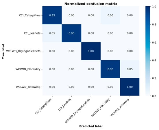
Figure 4.
Confusion matrix of the prediction results.
To solve the problem of overfitting, the image was preprocessed, including operations such as image scaling, rotation, and cropping. Batch normalization layers and a dropout were added to the network. The batch normalization layer normalizes the data to make the network more robust to changes in the distribution of the input data, thereby improving the model’s generalization ability.
3.1. Comparison of Model Performance
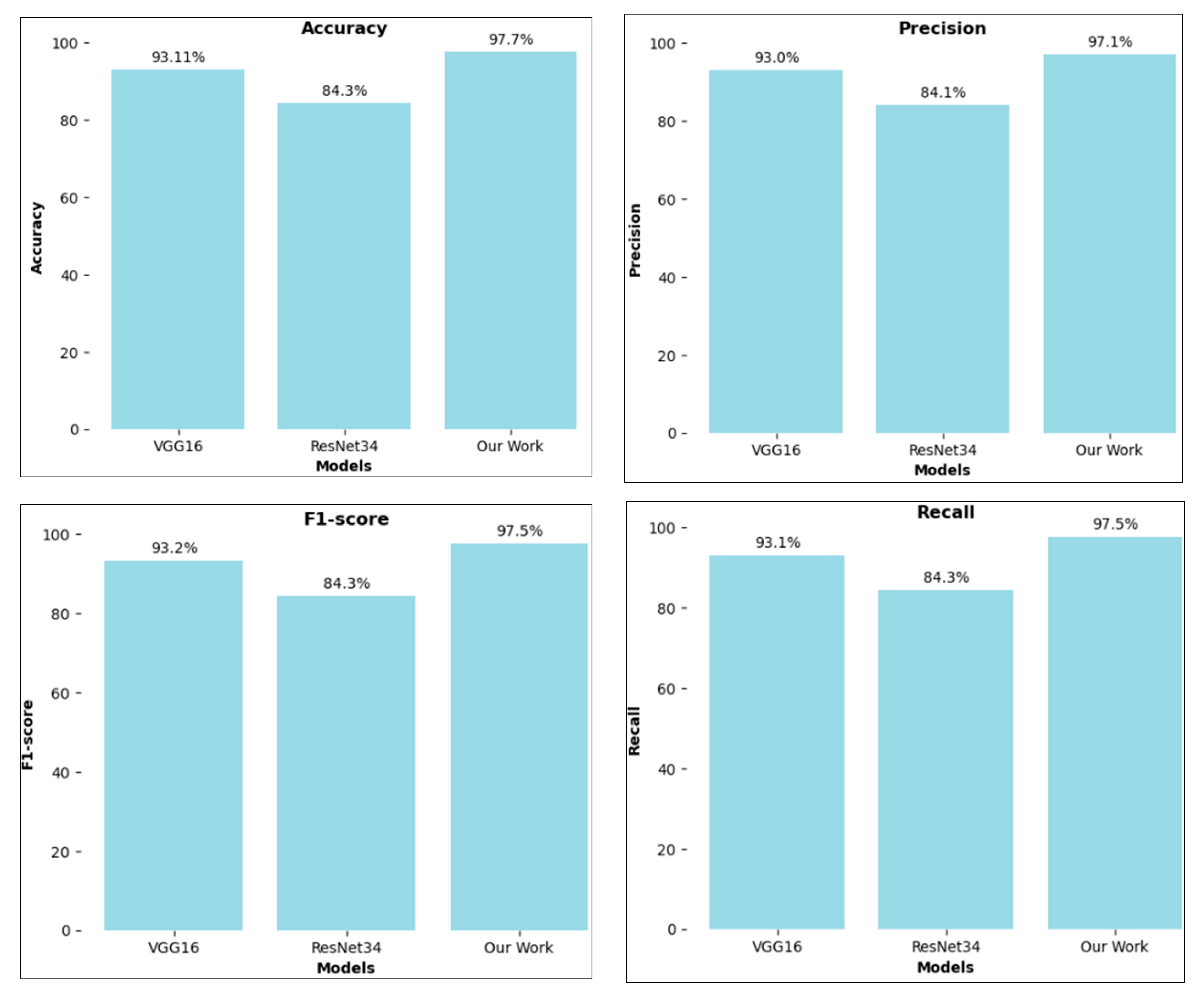
For comparison, we also used two models, ResNet-34 and vgg16. When contrasting ResNet-34 and vgg16, we observed that vgg16 achieved an accuracy of 93.11%, ResNet-34 achieved an accuracy of 84.30%, and the proposed model achieved an accuracy of 97.70%, as shown in Figure 5, Table 2 and Table 3. For comparison, we also used two models, ResNet-34 and vgg16.
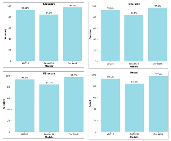
Figure 5.
Recognition accuracy, precision, f1-score, and recall of different models.
Table 2.
Classification performance comparison among different models.
Table 3.
Comparison of the training parameters and time.
3.2. Convergence Rate Analysis
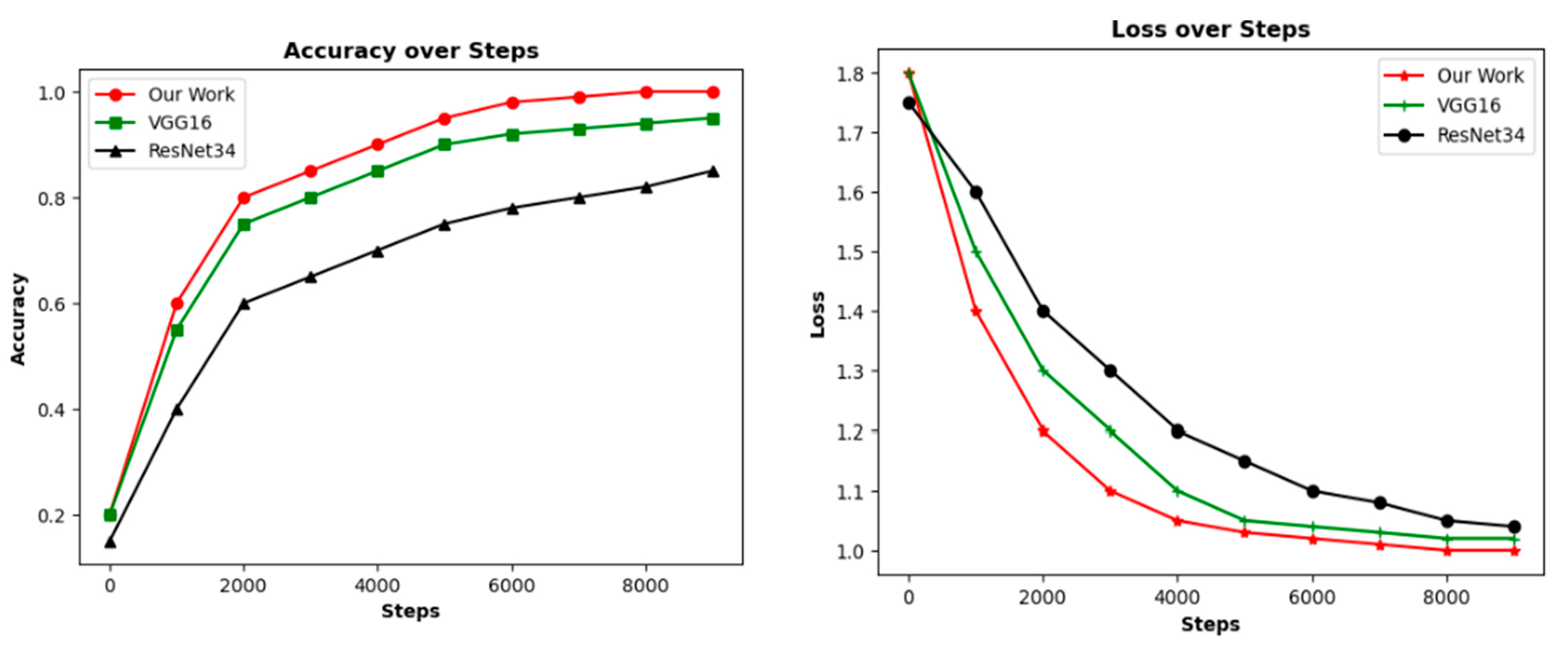
In this study, the loss value was computed using cross-entropy. The accuracy and loss values of the three models obtained during training are displayed in Figure 6. The experimental findings indicate that ResNet-34 converged at a quicker rate than VGG16. The convergence time necessary for training our model was comparable to that of ResNet-34, which is superior to VGG16.
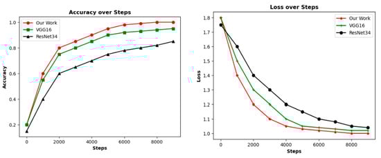
Figure 6.
Convergence comparison.
3.3. Training Time and Training Parameters
The number of parameters for each model and the training time necessary for the model to reach a stable state are presented in Table 3. The classical VGG16 model had the greatest number of parameters and the most time-consuming training process, while ResNet-34 had the shortest training time. The enhanced model exhibited a reduction of 120,864,099 training parameters when compared to the initial VGG16 model. The comprehensive performance of the convolutional neural network proposed in this paper is superior to that of all other models, as determined by its training parameters and training duration.
4. Conclusions
This paper presents a novel convolution neural network model that is an enhanced version of the VGG16 architecture. To reduce training parameters and accelerate convergence, the classifier of the traditional VGG16 network is modified by incorporating a batch normalization layer, a global average pooling layer, and a completely connected layer. The experimental outcomes demonstrate that the model assessment accuracy can attain a value of 97.70% following 103,832 s of training. The improvement in accuracy can help farmers detect plant diseases on time and take appropriate measures. In contrast to the traditional VGG16 network, the proposed approach results in a 120,864,099 parameter reduction and a 4.92 percent improvement in accuracy. While the training period for our model is more extensive in comparison to that of ResNet, it yields greater accuracy and has fewer parameters. The convolutional neural network that is efficiently and precisely designed to classify various categories of diseases in coconuts provides a workable method for disease identification. Further enhancements to our work are as follows: (1) expanding the collection of images, augmenting the quality of the datasets, and refining the training of the models; (2) the integration of Convolutional Neural Networks (CNNs) and autoencoders can improve recognition accuracy. Therefore, experimentation with advanced architectures like vision transformers to augment the recognition speed and accuracy is recommended.
Author Contributions
Conceptualization, X.H.; Methodology, X.H., M.M.A. and Y.F.; Software, X.H. and M.M.A.; Validation, X.H. and M.M.A.; Formal analysis, X.H. and M.M.A.; Investigation, M.M.A.; Resources, Y.F.; Writing—original draft, X.H. and Y.F.; Writing—review & editing, M.M.A., S.B.G. and Z.D.; Project administration, M.M.A., S.B.G. and Z.D. All authors have read and agreed to the published version of the manuscript.
Funding
This research received no external funding.
Data Availability Statement
The original contributions presented in this study are included in the article. Further inquiries can be directed to the corresponding authors.
Conflicts of Interest
The authors declare no conflict of interest.
References
- Divyanth, L.; Ahmad, A.; Saraswat, D. A two-stage deep-learning based segmentation model for crop disease quantification based on corn field imagery. Smart Agric. Technol. 2023, 3, 100108. [Google Scholar] [CrossRef]
- Li, J.; Yin, Z.; Li, D.; Zhao, Y. Negative contrast: A simple and efficient image augmentation method in crop disease classification. Agriculture 2023, 13, 1461. [Google Scholar] [CrossRef]
- Kurmi, Y.; Gangwar, S. A leaf image localization-based algorithm for different crops disease classification. Inform. Process. Agric. 2022, 9, 456–474. [Google Scholar] [CrossRef]
- Kundu, N.; Rani, G.; Dhaka, V.S.; Gupta, K.; Nayaka, S.C.; Vocaturo, E.; Zumpano, E. Disease detection, severity prediction, and crop loss estimation in MaizeCrop using deep learning. Artif. Intell. Agric. 2022, 6, 276–291. [Google Scholar] [CrossRef]
- Gogoi, M.; Kumar, V.; Begum, S.A.; Sharma, N.; Kant, S. Classification and detection of rice diseases using a 3-stage CNN architecture with transfer learning approach. Agriculture 2023, 13, 1505. [Google Scholar] [CrossRef]
- Zhang, L.; Ding, G.; Li, C.; Li, D. DCF-Yolov8: An improved algorithm for aggregating low-level features to detect agricultural pests and diseases. Agronomy 2023, 13, 2012. [Google Scholar] [CrossRef]
- Li, W.; Chen, P.; Wang, B.; Xie, C. Automatic localization and count of agricultural crop pests based on an improved deep learning pipeline. Sci. Rep. 2019, 9, 7024. [Google Scholar] [CrossRef] [PubMed]
- Ramachandran, P.; Zoph, B.; Le, Q.V. Searching for Activation Functions. arXiv 2017, arXiv:1710.05941. [Google Scholar] [CrossRef]
- Agarap, A. Deep learning using rectified linear units (relu). arXiv 2018, arXiv:1803.08375. [Google Scholar] [CrossRef]
- Krizhevsky, A.; Sutskever, I.; Hinton, G.E. ImageNet classification with deep convolutional neural networks. In Proceedings of the International Conference on Neural Information Processing System, Lake Tahoe, NV, USA, 3–6 December 2012; pp. 1097–1105. [Google Scholar]
- Szegedy, C.; Liu, W.; Jia, Y.; Sermanet, P.; Reed, S.; Anguelov, D.; Erhan, D.; Vanhoucke, V.; Rabinovich, A. Going deeper with convolutions. In Proceedings of the IEEE Conference on Computer Vision and Pattern Recognition, Boston, MA, USA, 7–12 June 2015; pp. 1–9. [Google Scholar]
- He, K.; Zhang, X.; Ren, S.; Sun, J. Deep residual learning for image recognition. In Proceedings of the IEEE Conference on Computer Vision and Pattern Recognition, Las Vegas, NV, USA, 27–30 June 2016; pp. 770–778. [Google Scholar]
- Zhu, J.Y.; Park, T.; Isola, P.; Efros, A.A. Unpaired image-to-image translation using cycle-consistent adversarial networks. In Proceedings of the IEEE International Conference on Computer Vision, Venice, Italy, 22–29 October 2017; pp. 2223–2232. [Google Scholar]
- Yang, G.; Tang, B.; Cao, S. Research on small sample image recognition based on transfer learning. J. Phys. Conf. Ser. 2019, 1302, 032039. [Google Scholar] [CrossRef]
- Yu, Y.; Lin, H.; Meng, J.; Wei, X.; Guo, H.; Zhao, Z. Deep transfer learning for modality classification of medical images. Information 2017, 8, 91. [Google Scholar] [CrossRef]
- Taylor, M.E.; Stone, P. Transfer learning for reinforcement learning domains: A survey. J. Mach. Learn. Res. 2009, 10, 1633–1685. [Google Scholar]
- Zhuang, F.Z.; Luo, P.; He, Q.; Shi, Z.Z. Survey on Transfer Learning Research. J. Softw. 2015, 26, 26–39. [Google Scholar] [CrossRef]
- Mnih, V.; Badia, A.P.; Mirza, M.; Graves, A.; Lillicrap, T.P.; Harley, T.; Silver, D.; Kavukcuoglu, K. Asynchronous Methods for Deep Reinforcement Learning. arXiv 2016, arXiv:1602.01783. [Google Scholar] [CrossRef]
- Simonyan, K.; Zisserman, A. Very deep convolutional networks for large-scale image recognition. arXiv 2014, arXiv:1409.1556. [Google Scholar] [CrossRef]
- Guo, R.; Shi, X.P.; Jia, D.K. Learning a deep convolutional network for image super-resolution reconstruction. J. Eng. Heilongjiang Univ. 2018, 9, 52–59. [Google Scholar] [CrossRef]
- Ruder, S. An overview of gradient descent optimization algorithms. arXiv 2016, arXiv:1609.04747. [Google Scholar] [CrossRef]
- Yan, Q.; Yang, B.; Wang, W.; Wang, B.; Chen, P.; Zhang, J. Apple leaf diseases recognition based on an improved convolutional neural network. Sensors 2020, 20, 3535. [Google Scholar] [CrossRef] [PubMed]
- Megalingam, R.K.; Aryan, K.; Gopika, A.; Jogesh, G.; Kunnambath, A.R.; Kota, A.H. Deep Learning Approach to Identify Pests in Coconut Trees. In Proceedings of the 2024 3rd International Conference for Innovation in Technology (INOCON), Bangalore, India, 1–3 March 2024. [Google Scholar] [CrossRef]


Disclaimer/Publisher’s Note: The statements, opinions and data contained in all publications are solely those of the individual author(s) and contributor(s) and not of MDPI and/or the editor(s). MDPI and/or the editor(s) disclaim responsibility for any injury to people or property resulting from any ideas, methods, instructions or products referred to in the content. |
© 2025 by the authors. Licensee MDPI, Basel, Switzerland. This article is an open access article distributed under the terms and conditions of the Creative Commons Attribution (CC BY) license (https://creativecommons.org/licenses/by/4.0/).