SPH Simulation of Gear Meshing with Lubricating Fluid–Solid Coupling and Heat-Transfer Process

Abstract

This study employs the meshfree Smoothed Particle Hydrodynamics (SPH) method to simulate the fluid–solid coupling process of gear meshing rotation with lubricating oil or oil jet lubrication fluids, considering the heat-transfer process under preset initial temperature conditions. While traditional grid methods face challenges in simulating the dynamic interaction between gear-meshing rotation and lubricating fluids, such as time-dependent contact in fluid–solid coupling and heat transfer, difficulties in handling meshing gaps, and the complexity of dynamic mesh setup, our approach leverages the unique advantages of meshless methods. In the established fluid–solid–heat coupling model, gears are considered as rigid bodies, and both fluids and gears are discretized into SPH particles, achieving fluid–solid coupling through the interaction between fluid particles and solid SPH particles. The model considers three cooling scenarios: oil pool cooling, oil jet cooling, and combined cooling. Simulation results show that oil pool cooling is more effective than oil jet cooling, but oil jet cooling can achieve localized spot cooling. The model exhibits good computational stability and efficiency in simulating the fluid–solid coupling and heat-transfer processes of gear rotation, oil jetting, and oil pool fluids. This study provides an effective numerical simulation method for gear lubrication cooling and has significant application potential for simulating complex scenarios such as gear operation and oil pool sloshing in coal mining machine arms. Compared to previous SPH work, this study couples a thermodynamic model in the simulation, thus enabling the modeling of fluid–thermal–solid coupled processes.

1. Introduction

Gear-meshing rotation is typically accompanied by interactions with lubricating oil or oil jet lubrication fluids, and simulating such problems using conventional grid methods poses significant challenges [1,2,3]. Firstly, gear meshing is a dynamic process involving time-dependent contact and load variations, which requires simulations to handle a large amount of transient data, challenging computational resources, and algorithm efficiency [4]. Secondly, the issue of fluid–solid coupling and heat transfer across large time scales also needs to be addressed, meaning that heat exchange between fluids and solids must be simulated on different time scales, increasing computational complexity [5]. For conventional CFD simulation methods, grid refinement can improve simulation accuracy but also increases computational load. In the simulation of gear meshing and lubricating oil fluid–solid coupling, it is necessary to ensure computational efficiency while capturing key physical phenomena accurately with the grid [6]. The treatment of meshing clearance is also a critical issue; due to the extremely small clearance between gears, it poses significant difficulties for fluid domain grid division, and too small a clearance can cause severe distortion during mesh reconstruction in the meshing area, leading to non-convergence in calculations [7,8]. Finally, the setup of moving grids is also a challenge because the rotational motion of gears requires the use of moving grid technology for simulation, which demands higher accuracy in grid reconstruction and computational stability [9].

Meshless methods show unique advantages in dealing with such problems, such as Moving Least Squares (MLS) method [10,11], Smoothed Particle Hydrodynamics (SPH) method [12,13,14,15], and Material Point Method (MPM) [16,17]. Compared to traditional grid methods, meshless methods only require the solution domain to be discretized with a set of nodes without the need for connection information between nodes, thus avoiding the difficulty of generating complex three-dimensional structure grids, facilitating the analysis of complex three-dimensional structures. The grid dependency of meshless approximation functions is very weak, and they do not deform or require re-meshing when analyzing problems with large deformations, moving interfaces, and discontinuities [18]. Meshless methods, such as the SPH method, use a finite number of particles with position and velocity characteristics to represent the fluid, and simulate the fluid as a whole through the particle method [19]. It is a Lagrangian form of meshless computation method, which eliminates the complex pre-processing and grid reconstruction and updating processes during computation and has the advantage of easily tracking and capturing large deformations and strongly nonlinear free surfaces [20]. Therefore, meshless methods provide an effective alternative in simulating gear meshing rotation fluid–solid coupling, especially for complex problems that are difficult to solve with grid methods [21]. Ji et al. [22] conducted numerical simulations of oil flow in a gearbox using the SPH method, comparing the results with experimental PIV data and analyzing the flow field behavior, capturing flow structures, splashing, and recirculation areas with good agreement. Keller et al. [23] examines oil-jet impingement on a rotating spur gear using the SPH method, demonstrating the efficiency of single-phase SPH for computational speed and accurately predicting flow phenomena, including the impact of jet inclination angles on oil spreading and splashing. Groenenboom et al. [24] introduces a coupled SPH–FE software tool (VPS, Virtual Performance Solution) for dynamic fluid flow and fluid–structure interaction simulations, highlighting its suitability for violent flow phenomena and validating its accuracy through applications including gear box simulation. The above studies indicate that SPH, as a mesh-free method, is well-suited for simulating fluid–structure interaction problems involving gears.

These SPH models have demonstrated advantages and are well-suited for problems involving free surface flows [25,26] and complex structural fluid-structure interactions [27]. Additionally, they have potential applications in complex multi-physics coupling problems that consider phenomena such as heat transfer [28,29]. Therefore, this paper takes into account the actual working scenario of gears, incorporating heat transfer into the modeling process to simulate the complex behavior of fluid–structure interaction and heat transfer during gear meshing and rotation with lubricating oil. This study uses the meshless SPH method to simulate the fluid–solid coupling process of gear meshing rotation and oil pool and oil jet lubrication fluids, while considering the heat transfer process under preset initial temperature conditions, and constructs a fluid–solid–heat coupling calculation model based on the SPH method. In the content of this chapter, Section 2 introduces the coupling model and its equations, Section 3 introduces the numerical solution process of the coupling model, and Section 4 introduces the simulation results and corresponding analysis.

2. Numerical Modeling Based on SPH

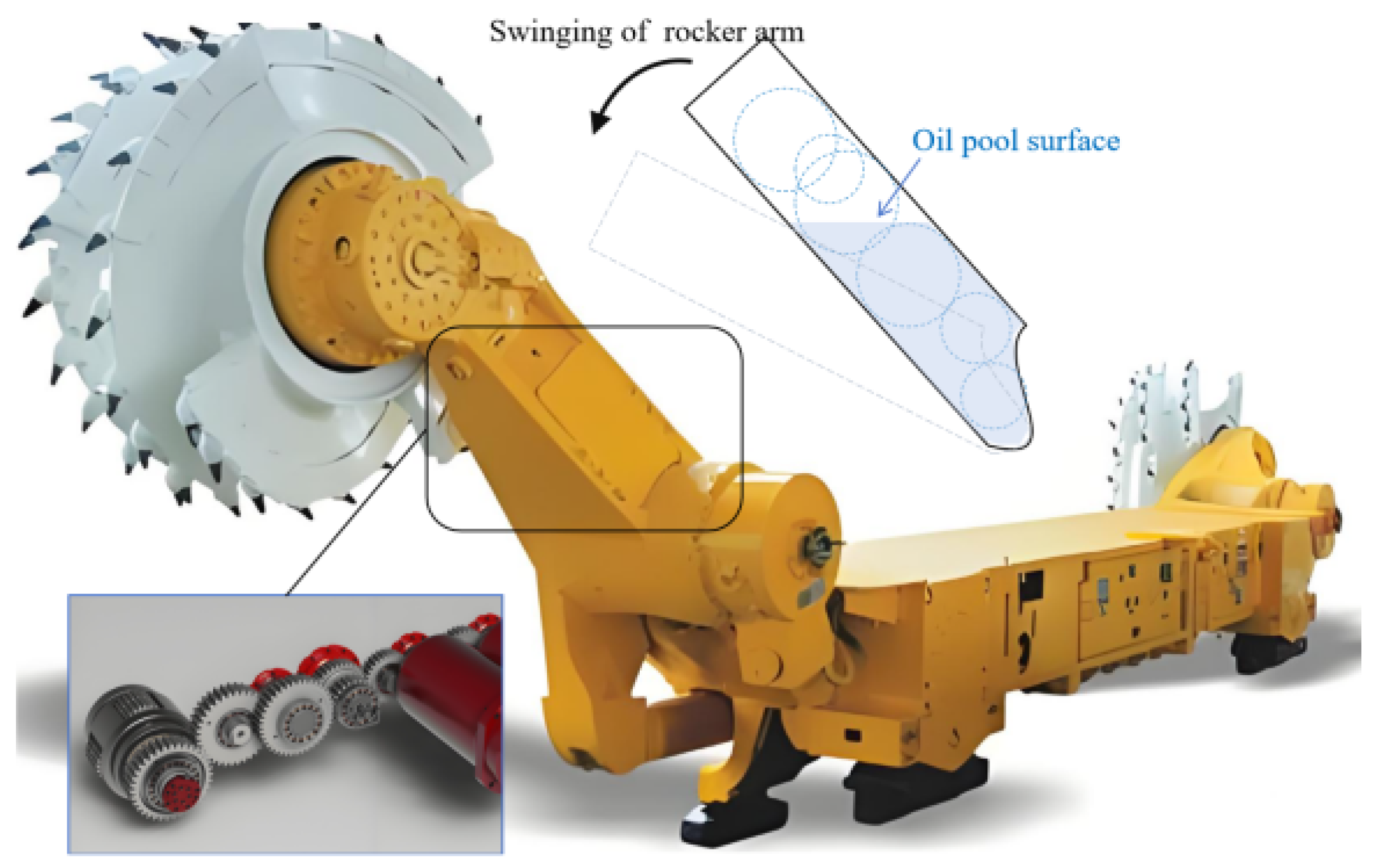
2.1. Model Description

As shown in Figure 1, this study establishes a Smoothed Particle Hydrodynamics (SPH) model for the coupling of gear meshing rotation, lubricant flow, and heat transfer. In Figure 1a, the different colors represent the boundary conditions (e.g., gears, lubricating oil). In Figure 1b, the different colors represent the gradient of the initial pressure distribution in the model. In the model, the large gear has 60 teeth, and the small gear has 45 teeth, with a corresponding transmission ratio of 0.75. The width of the oil pool is set to 0.8 m, and the height is set to 0.25 m. The immersion depth of the gears depends on the height of the liquid level in the oil pool. In the simulation of this paper, both the jet fluid and the oil pool fluid are discretized into uniformly distributed SPH particles with the same initial particle spacing, which is set to 1.5 mm. In this model, two types of lubricant cooling methods are considered: oil pool cooling and jet cooling, as well as a combined cooling method of both. For jet cooling, the lubricating oil is modeled as a jet, with an initial jet velocity given, under which the oil column impacts the moving gear surface at this initial velocity.

As shown in Figure 1, an inlet boundary condition is set at the top of the jet oil nozzle, which includes six rows of SPH particles with a given jet velocity. These particles update their positions according to the given velocity; when the movement of the top row of particles exceeds one particle spacing, a new row of SPH particles is injected at the fixed position at the top to simulate the continuous jet process. The lubricating oil for jet and oil pool cooling has the same properties, with a density set to 800 kg/m³ and a dynamic viscosity set to 10.0 mPa·s, both modeled using the weakly compressible fluid equation. Additionally, the two meshing gears are considered as rigid bodies, with their rotation speeds set according to the meshing speed of the gears. The gears are also discretized into SPH particles, and the positions and velocities of these particles are updated according to the rigid body motion, from which the linear velocity of any SPH particle constituting the gear can be obtained based on the gear’s rotational speed and the center of rotation. Furthermore, to consider the heat exchange process between the gears and the lubricating oil, both the fluid and the solid are modeled using thermodynamic equations to calculate heat transfer, simulating the heat-transfer behavior within the lubricating oil, within the gears, and between the lubricating oil and the gears.

2.2. Governing Equations of Fluid Dynamics

The fluid part includes both jet fluid and oil pool fluid, both of which are set as oils with the same properties. The oil density is set to 800 kg/m³, and the dynamic viscosity is set to 0.01 Pas. A weakly compressible SPH equation is used to establish the fluid dynamics model. In the weakly compressible SPH model, the fluid is assumed to be a medium with certain compressibility [30]. By controlling the value of the artificial speed of sound, the compressibility of the fluid is kept at a low level (the relative change in density does not exceed 1.0%), ensuring that the fluid’s motion behavior is similar to that of an incompressible fluid.

In the fluid model, the fluid is subject to free surface boundary conditions, without considering the effect of the gas phase. The governing equations for the fluid include the continuity equation and the momentum equation, expressed as follows:

$${\displaystyle \frac{d{\rho }_i}{dt}}={\sum }_{j=1}^{N_i}{m}_j\left({\mathit{v}}_i-{\mathit{v}}_j\right)·{\nabla }_{i}W\left({\mathit{x}}_i-{\mathit{x}}_j,h\right),$$

(1)

$${\displaystyle \frac{d{\mathit{v}}_i}{dt}}=-{\sum }_{j=1}^{N_i}{m}_j\left({\displaystyle \frac{p_i}{{\rho }_i^2}}+{\displaystyle \frac{p_j}{{\rho }_j^2}}\right){\nabla }_{i}W\left({\mathit{x}}_{ij},h\right)+{\sum }_{j=1}^{N_i}{\displaystyle \frac{{4m}_j\left({\mu }_i+{\mu }_j\right)}{{({\rho }_i+{\rho }_j)}^2}} {\displaystyle \frac{{\mathit{x}}_{ij}·{\nabla }_{i}W\left({\mathit{x}}_i-{\mathit{x}}_j,h\right)}{{\left|{\mathit{x}}_{ij}\right|}^2+{\left(0.01h\right)}^2}}{\mathit{v}}_{ij}+{\mathit{f}}_{\mathit{i}},$$

(2)

where t represents time, ρ is the fluid density, $\mathit{v}$ is the velocity vector, $\mathit{f}$ represents external forces or body forces, $p$ denotes fluid pressure, $\upsilon$ represents the kinematic viscosity of the fluid, i is the index for fluid particles, and j is the index for neighboring particles. ${\nabla }_{i}W\left({\mathit{x}}_{ij},h\right)$ is the value of the kernel gradient between particles i and j, where ${\mathit{x}}_{ij}$ is short for ${\mathit{x}}_i-{\mathit{x}}_j$; h is the smoothing length. In this paper, the smoothing length is a fixed value, taken as 1.2 times the particle spacing.

It should be noted that the fluid equations composed of Equations (11) and (12) are not closed and require the introduction of an equation of state to make these equations closed. The equation of state expresses the fluid pressure as a function of fluid density. This paper adopts the following form of the equation of state [31]:

$$p={\displaystyle \frac{{\mathrm{c}}^2{\rho }_0}{\gamma }}\left({\left({\displaystyle \frac{\rho }{{\rho }_0}}\right)}^{\gamma }-1\right),$$

(3)

where the coefficient = 7.0, c is the artificial speed of sound, taken as 10 times the maximum fluid velocity, $c=10V_{max}$. ${\rho }_0$ represents the initial density of the fluid phase (or reference density). Equation (3) provides an equation of state that ensures the weak compressibility of the fluid, meaning that small changes in density can lead to changes in pressure, thereby controlling further compression of the local fluid.

In the simulations, the impact of the jet on the gears is involved, and there are also complex interactions between the gears and the fluid in the oil pool. To ensure the numerical stability of the fluid simulation, it is necessary to introduce an artificial viscosity term into the momentum equation to suppress the numerical noise generated by the impact. This type of numerical noise is mainly manifested as noise in fluid pressure. The expression for the artificial viscosity term is [32]:

$${\Pi }_i^{art}=-{\sum }_{j=1}^{N_i}{m}_j{\pi }_{ij}^{art}{\nabla }_{i}W\left({\mathit{x}}_i-{\mathit{x}}_j,h\right),$$

(4)

$${\pi }_{ij}^{art}=\left\{\begin{array}{c}-\alpha {\displaystyle \frac{c{\phi }_{ij}}{{\overline{\rho }}_{ij}}} {\mathit{v}}_{ij}·{\mathit{x}}_{ij}<0\\ 0 {\mathit{v}}_{ij}·{\mathit{x}}_{ij}\ge 0\end{array}\right.,$$

(5)

where ${\overline{\rho }}_{ij}={\displaystyle \frac{{\overline{\rho }}_i+{\overline{\rho }}_j}{2}}$, ${\phi }_{ij}=h_{ij}{\displaystyle \frac{{\mathit{v}}_{ij}·{\mathit{x}}_{ij}}{{\left|{\mathit{x}}_{ij}\right|}^2+0.01h^2}}$, $\alpha =0.01$. From the above equation, it can be seen that the artificial viscosity force is not a true viscous force; it only acts when two particles are moving towards each other. Simulation results indicate that the introduction of this term can effectively suppress non-physical numerical noise effects.

After incorporating the artificial viscosity force, the fluid momentum equation is transformed into the following form:

$${\displaystyle \frac{d{\mathit{v}}_i}{dt}}=-{\sum }_{j=1}^{N_i}{m}_j\left({\displaystyle \frac{p_i}{{\rho }_i^2}}+{\displaystyle \frac{p_j}{{\rho }_j^2}}\right){\nabla }_{i}W\left({\mathit{x}}_{ij},h\right)+{\sum }_{j=1}^{N_i}{\displaystyle \frac{{4m}_j\left({\mu }_i+{\mu }_j\right)}{{\left({\rho }_i+{\rho }_j\right)}^2}} {\displaystyle \frac{{\mathit{x}}_{ij}·{\nabla }_{i}W\left({\mathit{x}}_i-{\mathit{x}}_j,h\right)}{{\left|{\mathit{x}}_{ij}\right|}^2+{\left(0.01h\right)}^2}}{\mathit{v}}_{ij}+{\Pi }_i^{art}+{\mathit{f}}_{\mathit{i}}.$$

(6)

2.3. Rigid Body Motion Equations

In the simulations, the motion of the gears is primarily rotational, described by the given meshing speed. Based on the overall rotational speed of the gears, the velocities and positions of the particles constituting the gears are updated using the motion relationship between the gear rigid body and the gear particles. The gears are discretized using two types of particles: boundary particles and internal particles. Boundary particles generate repulsive forces to prevent fluid particles from penetrating the rigid surface. Internal particles possess SPH particle properties, and through the interaction of internal particles with surrounding fluid particles, fluid–rigid body coupling is achieved.

Considering a more general case, the motion of a rigid body can be decomposed into translation of the center of mass and rotation about the center of mass, which can be described by Newton’s second law. The linear and angular accelerations of the rigid body are expressed as follows:

$${\displaystyle \frac{d{\mathit{V}}_I}{dt}}={\displaystyle \frac{{\mathit{F}}_I}{M_I}},$$

(7)

$${\displaystyle \frac{d{\mathbf{\Omega }}_I}{dt}}={\displaystyle \frac{{\mathit{T}}_I}{I_I}},$$

(8)

where ${\mathit{V}}_I$,${\mathbf{\Omega }}_I$ represent the linear velocity and angular velocity vectors of the I-th rigid body, respectively. ${\mathit{F}}_I$,${\mathit{T}}_I$ represent the external forces and torques acting on the rigid body. $M_I$,$I_I$ represent the mass and moment of inertia of the rigid body, respectively. If the internal space of the rigid body has been discretized into SPH particles, then the internal SPH particles can be treated as mass points to calculate the mass and moment of inertia of the rigid body, as shown in the following equations:

$$M_I={\sum }_i{m}_i,$$

(9)

$$I_I={\sum }_i{m}_i{\left({\mathit{r}}_i-{\mathit{R}}_I\right)}^2,$$

(10)

where i represents the i-th SPH particle within the rigid body, ${\mathit{r}}_i$ represents the position vector of particle i, and ${\mathit{R}}_I$ represents the position vector of the center of mass of rigid body. The position vector of the center of mass of rigid body I can be determined based on the positional information of the discrete SPH particles as follows:

$${\mathit{R}}_I={\displaystyle \frac{{\sum }_i{m}_i{\mathit{r}}_{\mathit{i}}}{{\sum }_i{m}_i}}.$$

(11)

The forces acting on a rigid body mainly consist of three types: forces generated by the fluid acting on the surface of the rigid body (including pressure and viscous forces), volume forces acting on the center of mass of the rigid body (including gravity), and forces resulting from collisions between rigid bodies. By summing the forces on the internal and boundary particles, the expressions for the total force and torque acting on the rigid body can be obtained as follows:

$$\left\{\begin{array}{c}{F}_{\mathrm{I}}={\sum }_{i=1}^{N_{I,interior}}{m}_i{\displaystyle \frac{d{v}_i}{dt}}+{\sum }_{i=1}^{N_{I,boundary}}{m}_i{\displaystyle \frac{d{v}_i}{dt}}\\ T_I={\sum }_{i=1}^{N_{I,interior}}{m}_i\left(x_i-X_I\right)\times {\displaystyle \frac{d{v}_i}{dt}}+{\sum }_{i=1}^{N_{I,boundary}}{m}_i\left(x_i-X_I\right)\times {\displaystyle \frac{d{v}_i}{dt}}\end{array}\right.,$$

(12)

where the subscript i represents the discrete particles that make up rigid body I, $N_I$ represents the number of discrete particles constituting rigid body; $m_i$ represents the mass of particle i, $x_i$ represents the position vector of particle, and $X_I$ represents the position vector of the center of mass of rigid body.

In the simulations of this paper, the motion of the gears under the influence of the fluid is not considered; the gears always move according to the given initial conditions and rotational speed. Therefore, based on the motion relationship between the gears and the particles that constitute the gears, the velocity of the gear particles at any moment can be determined by the following equation:

$$\left\{\begin{array}{c}{v}_{1i}=-{\mathbf{\Omega }}_{I1}\times \left(x_{1i}-X_{I1}\right)\\ v_{2i}=-{\mathbf{\Omega }}_{I2}\times \left(x_{2i}-X_{I2}\right)\end{array}\right..$$

(13)

where $v_{1i}$ and $v_{2i}$ represent the velocity vectors of particle on gears 1 and 2, respectively. ${\mathbf{\Omega }}_{I1}$ and ${\mathbf{\Omega }}_{I2}$ represent the angular velocity vectors of gears 1 and 2, respectively, and $X_{I1}$ and $X_{I2}$ represent the position vectors of particle on gears 1 and 2, respectively.

2.4. Governing Equations of Thermal Dynamics

This paper considers the heat-transfer processes within the gears, within the fluid, and between the fluid and gears, with the main form of heat transfer being conduction. Since the SPH method is a Lagrangian approach, each SPH particle carries physical quantities related to the fluid and thermodynamics, which naturally enables the convective heat transfer method. Therefore, the thermodynamic equation used in this paper is expressed as the derivative of the particle temperature with respect to time [14,33]:

$$c_{p,i}{\displaystyle \frac{d{T}_i}{dt}}={\sum }_{j=1}^{N_i}{\displaystyle \frac{{4m}_j}{{{\rho }_i\rho }_j}}{\displaystyle \frac{k_i{k}_j}{k_i+k_j}}\left(T_i-T_j\right){\displaystyle \frac{1}{\left|{\mathit{x}}_{ij}\right|}}{\displaystyle \frac{\partial W\left({\mathit{x}}_i-{\mathit{x}}_j,h\right)}{\partial \left|{\mathit{x}}_i-{\mathit{x}}_j\right|}},$$

(14)

where ${\mathit{x}}_{ij}$=${\mathit{x}}_i-{\mathit{x}}_j$, $k_i$ and $k_j$ are the thermal conductivity coefficients of the materials represented by particles i and j (particles i and j may represent fluid and solid particles, respectively); $T_i$ and $T_j$ are the temperatures of particles i and j.

3. Model Implementation and Numerical Solution

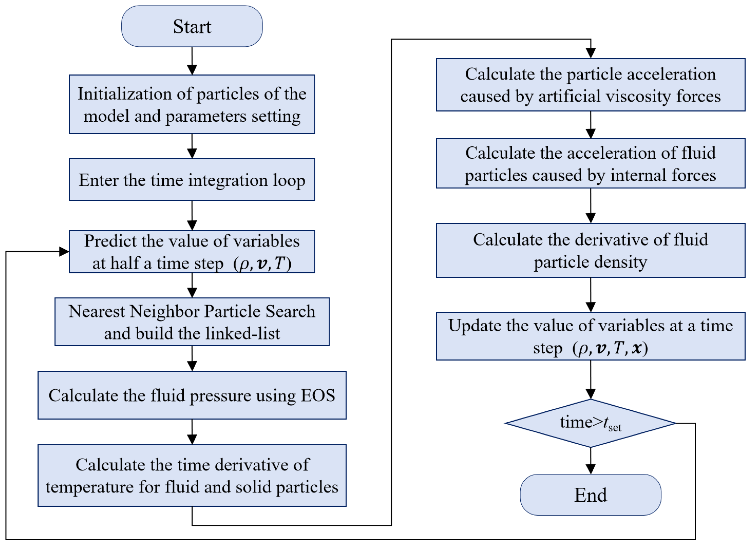
3.1. Numerical Solution Strategy

The fluid–solid–thermal coupling model established in this paper makes the following assumptions:

(1)

The gears are considered as rigid bodies, and their positions are updated according to the equations of rigid body rotation.

(2)

The gears are also discretized into SPH particles, which are used to discretize the thermodynamic equations. These particles possess physical properties such as temperature, mass, and density.

(3)

The fluid–solid coupling is achieved through the interaction between fluid particles and adjacent solid SPH particles (i.e., gear particles). The motion of the gears is according to the given rotational speed.

(4)

The thermal expansion characteristics of the oil and the variation of oil viscosity with temperature are not considered.

(5)

The heat dissipation of the gears to the air is not considered; only the heat exchange between the gears and the lubricating oil is considered, which is completed through the interaction between fluid particles and gear particles that support each other’s domains.

It should be noted that ignoring heat transfer through gears and air reduces the heat-dissipation effect of the gears. Moreover, the viscosity of lubricating oil generally decreases with increasing oil temperature, which is not conducive to the formation of oil films. However, since the main purpose of this study is to establish a numerical simulation framework for fluid–structure–thermal interactions, the related assumptions can be gradually improved on the basis of this framework in the future.

In our model, fluid and solid particles are treated as a continuous medium, and their interactions are governed by the same set of governing equations, such as the Navier_Stokes equations for fluid dynamics and the equations of motion for solid mechanics. The coupling is achieved by defining interaction forces between fluid and solid particles. These forces account for the pressure and viscous forces exerted by the fluid on the solid, as well as the reaction forces from the solid to the fluid. The SPH method allows for a straightforward evaluation of these forces by using a smoothing kernel to approximate the field quantities at the fluid–solid interface. This approach ensures that the fluid and solid particles can exchange momentum and energy effectively, leading to accurate simulations of fluid–solid interactions. Furthermore, the Lagrangian nature of SPH enables the model to track the motion of both fluid and solid particles without the need for a fixed grid, which simplifies the handling of complex geometries and dynamic interfaces. This capability is crucial for accurately simulating the dynamic behavior of fluid and solid systems, such as the interaction between lubricating fluids and rotating gears in our study.

Based on the fluid–solid–thermal coupling model established in Section 2, which includes fluid model, rigid body model, and thermodynamic model, the integrated set of governing equations is as follows:

$$\left\{\begin{array}{c}{\displaystyle \frac{d{\rho }_i}{dt}}={\sum }_{j=1}^{N_i}{m}_j\left({\mathit{v}}_i-{\mathit{v}}_j\right)·{\nabla }_{i}W\left({\mathit{x}}_i-{\mathit{x}}_j,h\right)+D_{ij}\\ \begin{array}{c}{\displaystyle \frac{d{\mathit{v}}_i}{dt}}=-{\sum }_{j=1}^{N_i}{m}_j\left({\displaystyle \frac{p_i}{{\rho }_i^2}}+{\displaystyle \frac{p_j}{{\rho }_j^2}}\right){\nabla }_{i}W\left({\mathit{x}}_{ij},h\right)+{\sum }_{j=1}^{N_i}{\displaystyle \frac{{4m}_j\left({\mu }_i+{\mu }_j\right)}{{({\rho }_i+{\rho }_j)}^2}} {\displaystyle \frac{{\mathit{x}}_{ij}·{\nabla }_{i}W\left({\mathit{x}}_i-{\mathit{x}}_j,h\right)}{{\left|{\mathit{x}}_{ij}\right|}^2+{\left(0.01h\right)}^2}}{\mathit{v}}_{ij}+{\Pi }_i^{art}+{\mathit{f}}_{\mathit{i}}\\ \begin{array}{c}{c}_{p,i}{\displaystyle \frac{d{T}_i}{dt}}={\sum }_{j=1}^{N_i}{\displaystyle \frac{{4m}_j}{{{\rho }_i\rho }_j}}{\displaystyle \frac{k_i{k}_j}{k_i+k_j}}\left(T_i-T_j\right){\displaystyle \frac{1}{\left|{\mathit{x}}_{ij}\right|}}{\displaystyle \frac{\partial W\left({\mathit{x}}_i-{\mathit{x}}_j,h\right)}{\partial \left|{\mathit{x}}_i-{\mathit{x}}_j\right|}}\\ D_{ij}=\beta {\sum }_{j=1}^N{V}_j{h}_{ij}{c}_{ij}{\Psi }_{ij}{\displaystyle \frac{\partial W_{ij}}{\partial x_i^{\beta }}}\end{array}\\ {\Pi }_i^{art}=-{\sum }_{j=1}^{N_i}{m}_j{\pi }_{ij}^{art}{\nabla }_{i}W\left({\mathit{x}}_i-{\mathit{x}}_j,h\right)\end{array}\\ {\displaystyle \frac{d{\mathit{x}}_i}{dt}}={\mathit{v}}_i\end{array}\right..$$

(15)

In the above system of equations, to ensure the stability of the model calculations, in addition to using the artificial viscosity term, a density dissipation term has also been used in the continuity equation, the specific form of which can be found in reference [32]. From the above equations, it is known that the system is expressed in the form of time derivatives of particles, including density derivatives, velocity derivatives (i.e., acceleration), and temperature derivatives. Once the time derivatives at the current time step are determined, an explicit time integration algorithm can be used to update the physical quantities of the corresponding particles, achieving the numerical solution of the coupled model.

The smoothing length is an important parameter in the SPH method, as it determines the number and distribution of particles within the influence domain. The choice of smoothing length significantly affects the simulation results: an excessively large smoothing length can lead to overly smooth results, thereby reducing the ability to capture details, while an excessively small smoothing length can result in computational instability and increased numerical noise. Therefore, choosing an appropriate smoothing length is crucial for improving the accuracy and stability of the simulation. In this study, we adjusted the values of the smoothing length to be 0.8, 1.2, and 2.0 times the particle spacing. The simulation results showed that when the smoothing length was 0.8, the computation was unstable. The temperature-distribution results obtained with particle spacings of 1.2 and 2.0 were essentially consistent, but the computation time for 2.0 was about twice as long.

3.2. Time Integration Scheme

The previous section presented the discrete equations for fluid flow and heat transfer control, which are expressed as a system of equations in terms of particle time derivatives and are solved using a time integration algorithm. In this paper, the Leap-frog method is used as the time integration algorithm, where the physical quantities such as velocity, temperature, and density of the particles are updated half a step ahead of the displacement within each time step. Within each time step, the variables are updated according to the following equations [34]:

$${\rho }_{n+1/2}={\rho }_{n-1/2}+{\left({\displaystyle \frac{d\rho }{dt}}\right)}_n·∆t,$$

(16)

$$v_{n+1/2}^{\alpha }=v_{n-1/2}^{\alpha }+{\left({\displaystyle \frac{d{v}^{\alpha }}{dt}}\right)}_n·∆t,$$

(17)

$$T_{n+1/2}^{\alpha }=T_{n-1/2}^{\alpha }+{\left({\displaystyle \frac{d{T}^{\alpha }}{dt}}\right)}_n·∆t,$$

(18)

$$x_{n+1}^{\alpha }=x_n^{\alpha }+v_{n+1/2}^{\alpha }·∆t,$$

(19)

where $∆t$ represents the time step size, which is determined by the Courant–Friedrichs–Lewy (CFL) condition; $n$ represents the current time step.

According to the CFL criterion, the time step size must satisfy the following condition [14,34]:

$$\left\{\begin{array}{c}{∆t}_c\le 0.1{\mathrm{m}\mathrm{i}\mathrm{n}}_i\left({\displaystyle \frac{h}{c+\left|{\mathit{v}}_i\right|}}\right)\\ {∆t}_T\le 0.1{\mathrm{m}\mathrm{i}\mathrm{n}}_i\left({\displaystyle \frac{{\rho }_i{c}_{pi}{h}^2}{k_i}}\right)\end{array}\right..$$

(20)

where ${∆t}_{\mathrm{c}}$ and ${∆t}_{\mathrm{T}}$ are the maximum time step values derived from the flow and heat transfer characteristics, respectively. In actual computations, the minimum of the two values should be chosen; $c_{pi}$ represents the specific heat capacity of particle i, and $k_{\mathrm{i}}$ represents the thermal conductivity of particle.

Based on the numerical solution algorithm using the Leap-frog method, a numerical calculation flow as shown in Figure 2 has been formed. This paper has compiled a computation code based on the FORTRAN language according to this flow and uses this code to complete the numerical calculations for the subsequent chapters of the paper. Figure 3 provides a structural diagram of the FORTRAN program, as well as the calling relationships between various sub-function files. The header file module ‘configuration.f90’ is set up, which provides the public variables and data required during the program execution. The main program file is ‘source.f90’, which calls the initialization function and the time integration function. Most of the program-execution process is completed in the ‘time integration’, where the ‘single step’ function calculates the various time derivatives of the particles, and the ‘output’ function outputs the calculation results of the particles at a set time interval, which can be imported into Tecplot for post-processing and display. The function ‘refresh jet inlet’ is mainly used to implement the jet inlet boundary condition, periodically injecting a row of SPH particles into the jet oil column and adjusting the index order of particles in the calculation domain.

4. Results and Analysis

Utilizing the established fluid–solid–thermal coupling model, the paper simulates the gear rotation and heat-transfer cooling process under three cooling conditions, including oil pool cooling, jet cooling, and combined cooling. It is assumed that the gears have an initial temperature, which is uniformly distributed at 60 °C (333 K); the initial temperature of the oil pool and jet oil is set to 20 °C (293 K). For oil pool cooling, under the initial conditions, there is a temperature difference between the oil pool fluid and the gears, and heat will be conducted from the gears to the fluid.

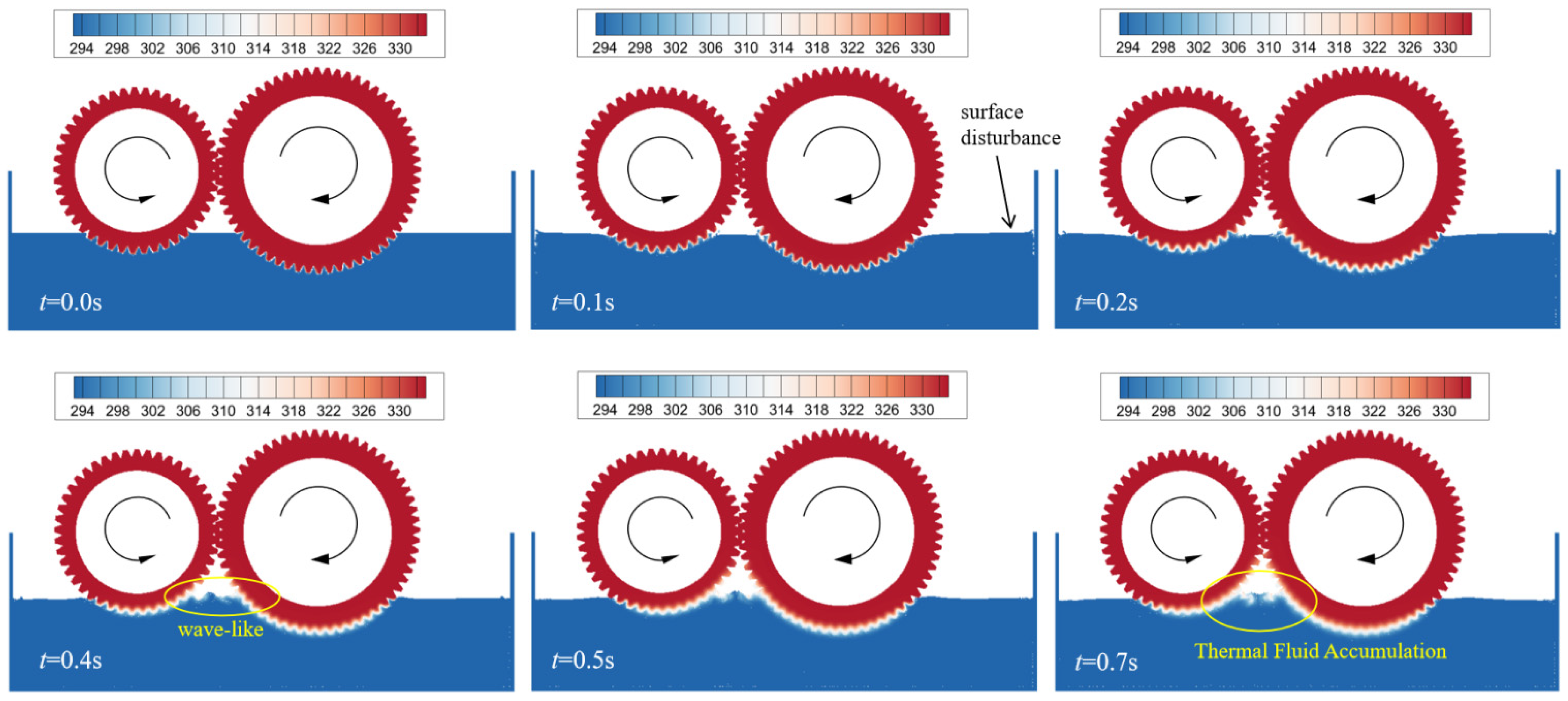
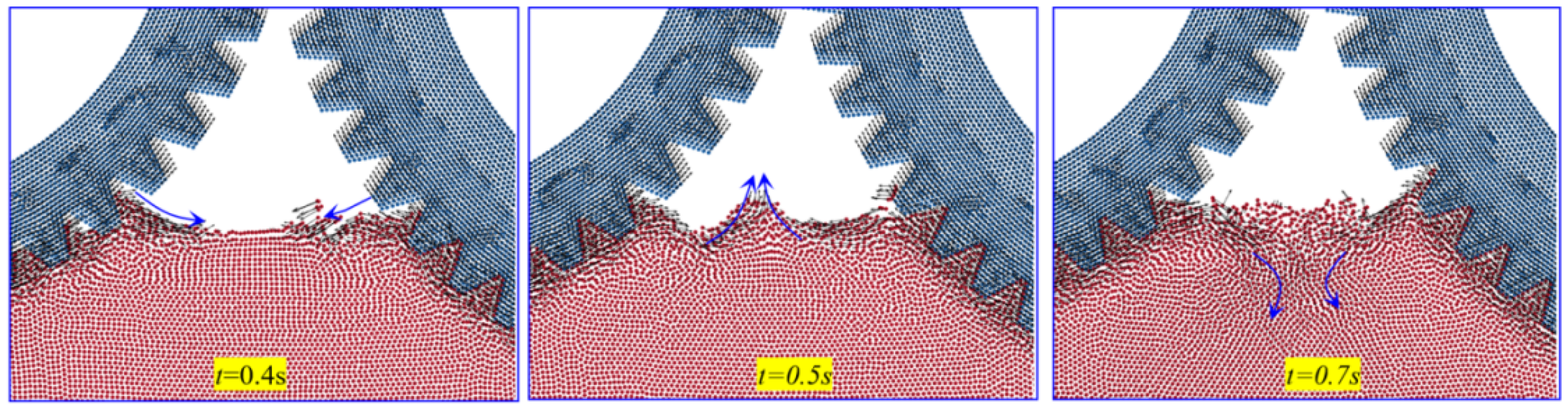
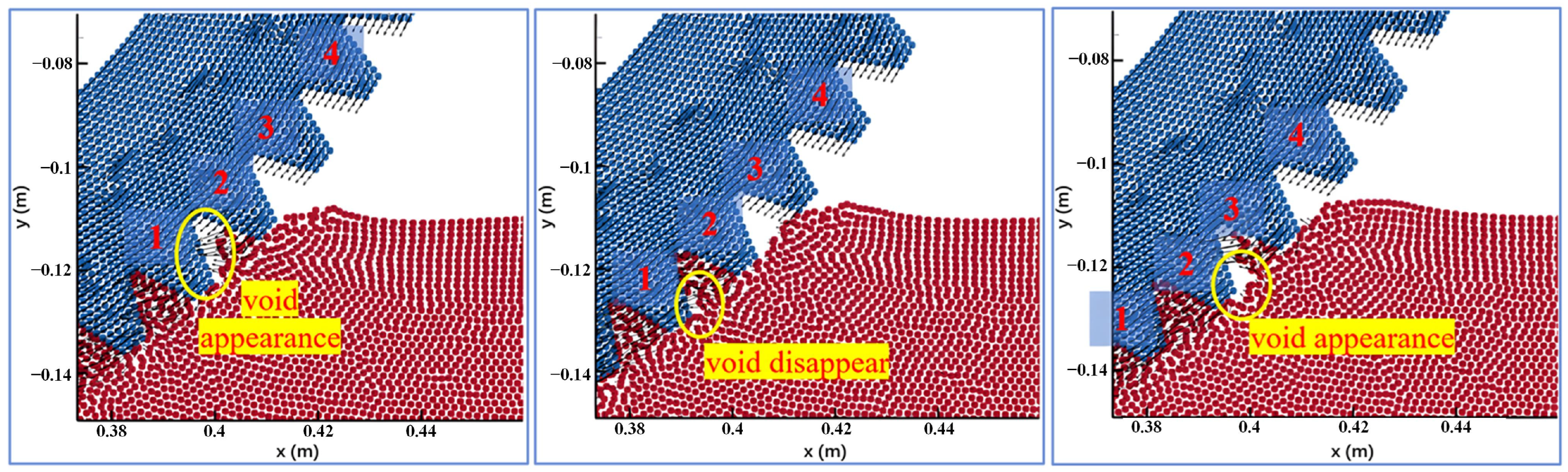
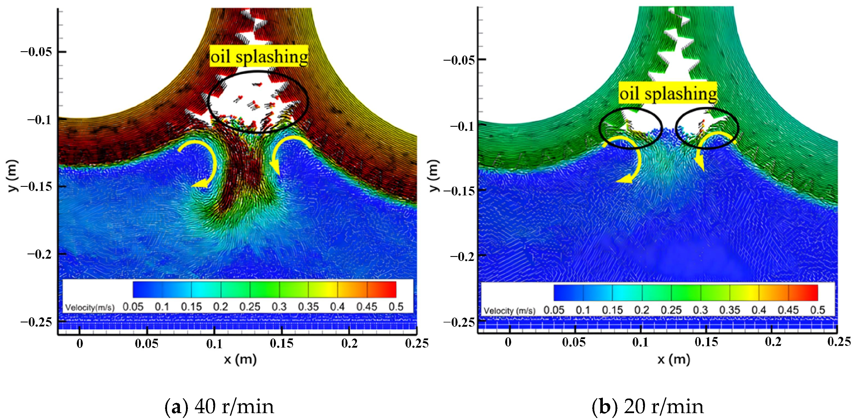
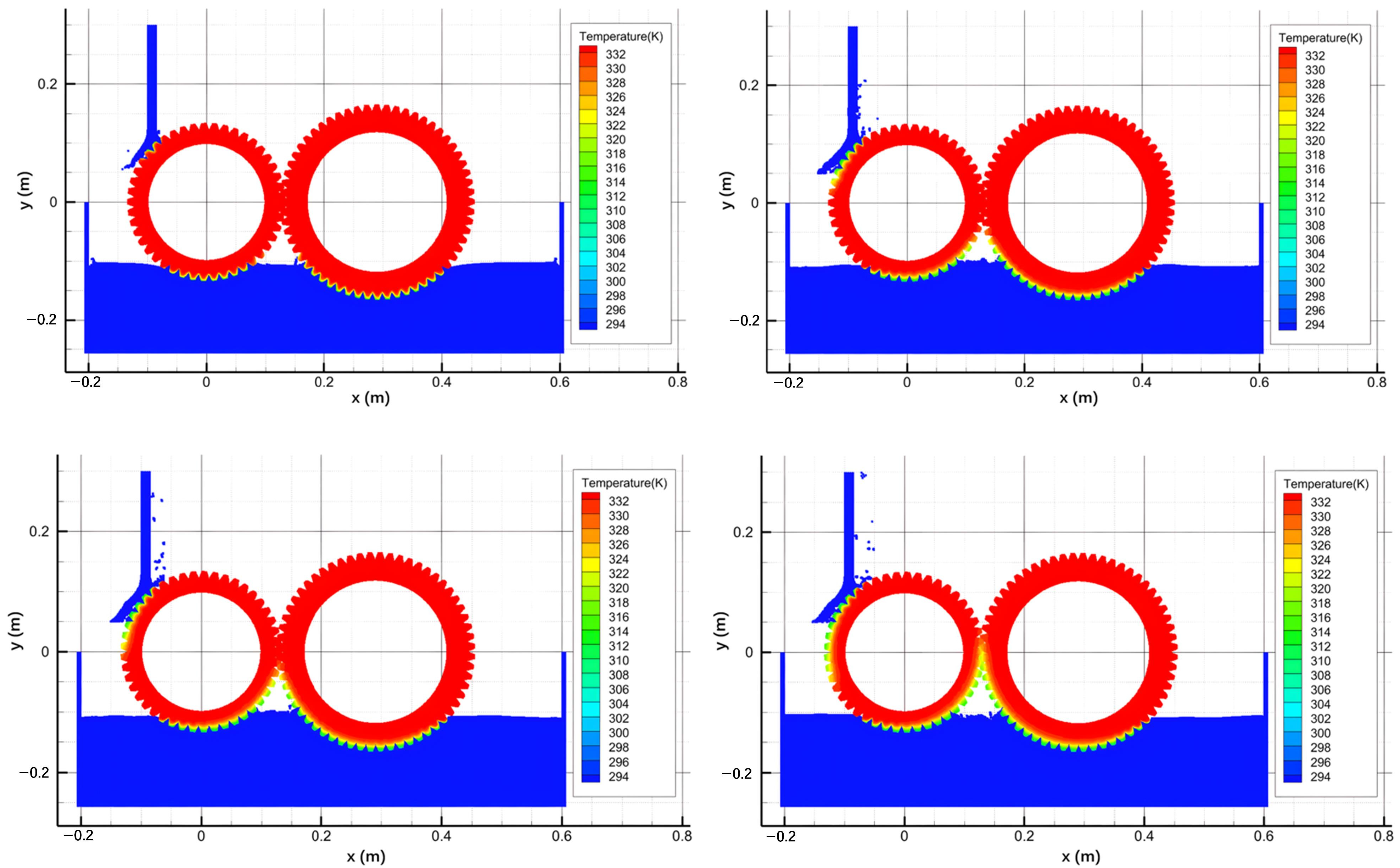
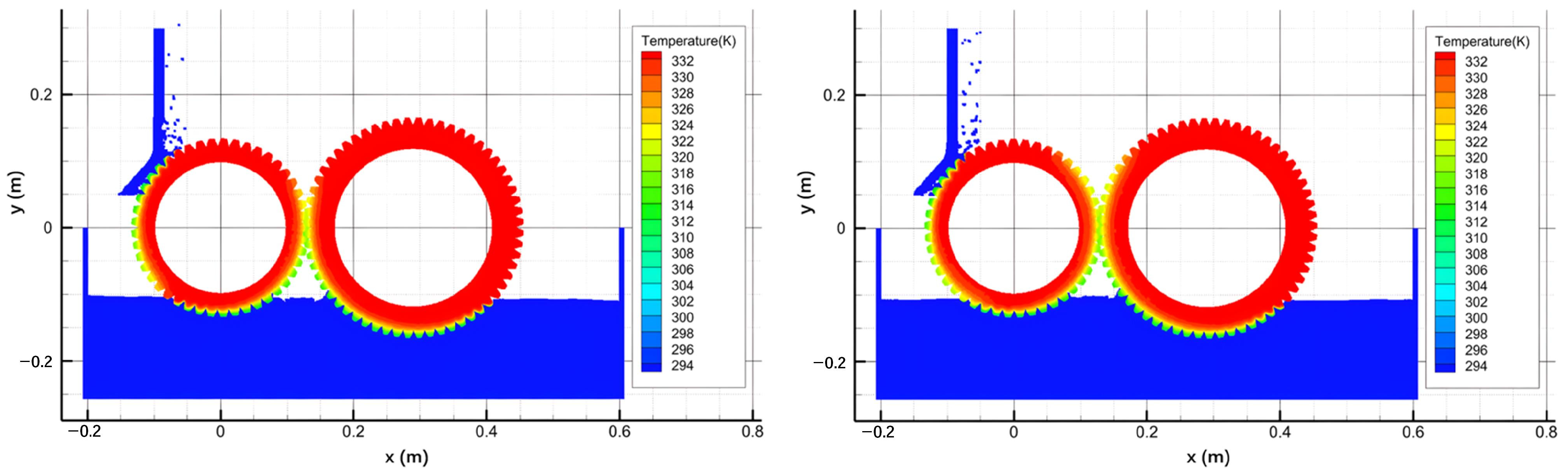
4.1. Results of Transmission Gear with Oil Pool Cooling

Figure 4 presents the simulation results of oil pool cooling when the depth of the oil pool is 0.15 m. This example utilized a total of 75,000 SPH particles, including fluid particles, solid particles, and boundary particles. The time step was set to 0.00001 s, and the simulation ran for 70,000 steps, corresponding to a physical time of 0.7 s. As shown in the figure, at the initial moment, there is a 40 °C temperature difference between the oil pool and the gears. As the gears rotate and heat transfer proceeds, the temperature near the gear surface decreases. Gear 1 is set to rotate at 20 revolutions per minute (rpm), and Gear 2 at 15 rpm. Since the gear speeds are loaded onto the gears at the start of the calculation, the significant speed difference causes slight fluctuations on the oil pool surface. In Figure 5, the blue arrows represent the direction of fluid particle movement. As shown in Figure 4 and Figure 5, the meshing rotation of the gears causes the fluid to converge towards the middle position between the two gears, demonstrating wavy motion behavior between the gears. The heat from the gears is transferred to the oil in the oil pool through heat conduction, and the stirring of the oil by the two gears causes the oil to gather in the middle between the gears, making the temperature of the oil in the middle between the two gears significantly higher than in other locations.

Figure 6 presents the simulation results of the fluid motion behavior when the gear rotates into the liquid surface. The numbers in Figure 6 represent the gear tooth numbers. As shown in the figure, after rotating into the liquid surface, a portion of “gas” (i.e., a cavity) is trapped between the first and second teeth. As the depth of rotation increases, the cavity gradually disappears, which can be attributed to the increase in fluid pressure compressing the gas volume and causing it to decrease. The same process of cavity formation and disappearance is also experienced between the second and third teeth. However, it should be noted that the model in this paper assumes the fluid has a free surface boundary condition and does not consider the presence of gas.

Figure 7 compares the simulation results of the fluid behavior between the gears at two different gear rotation speeds. The yellow arrows in Figure 7 represent the direction of fluid particle movement. From the figure, it can be seen that as the speed of the smaller gear increases from 20 rpm to 40 rpm, the degree of splashing at the gear interface also increases; after the fluid “accumulates” in the middle, two counter-rotating vortices are formed at the lower part of the liquid surface due to the backflow, and these vortices become more pronounced with the increase in rotation speed. This phenomenon indicates that the rotation speed of the gears has a significant impact on the fluid splash behavior; an increase in speed enhances the dynamic behavior of the fluid, leading to a more complex flow field distribution and a stronger splash effect.

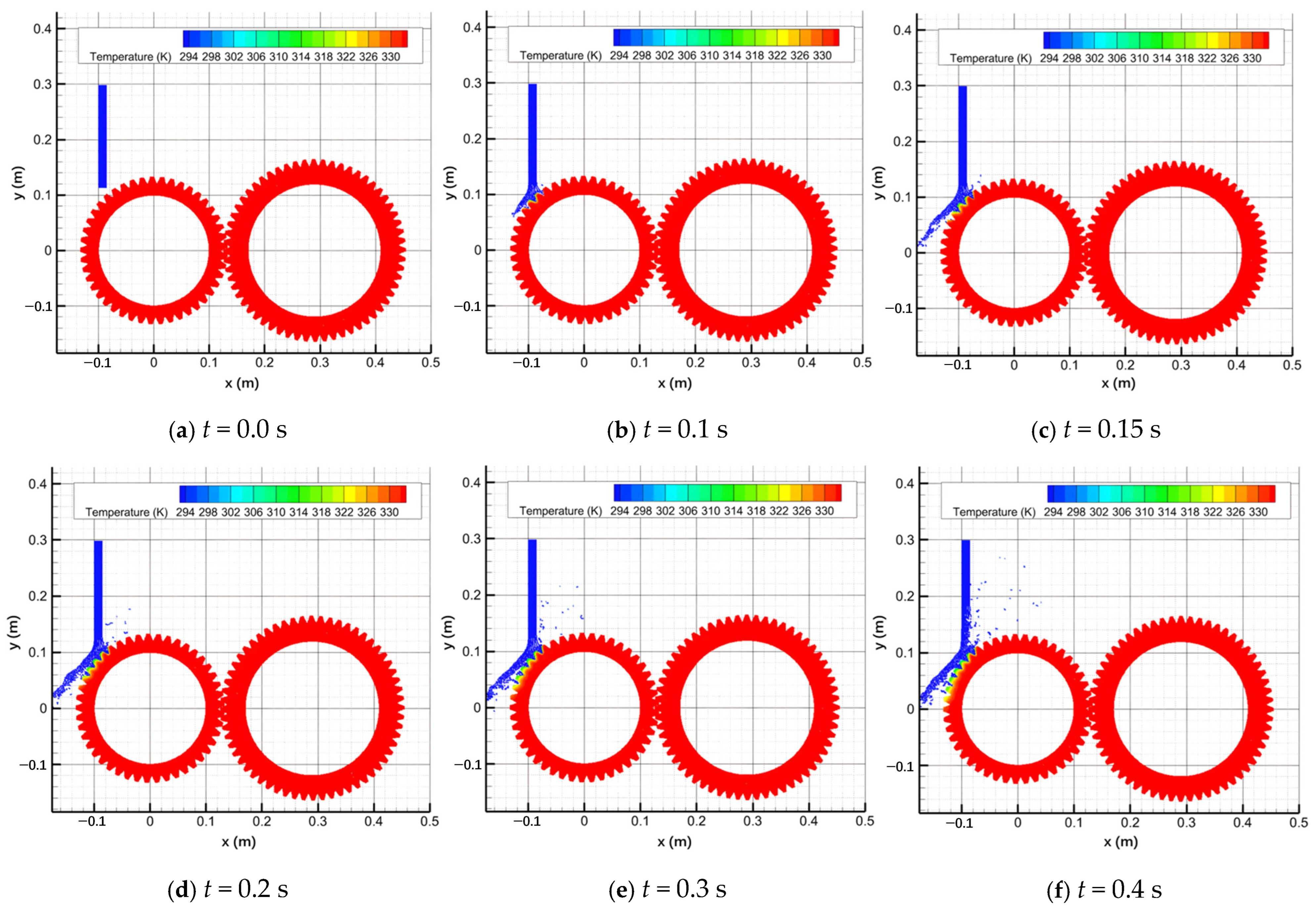
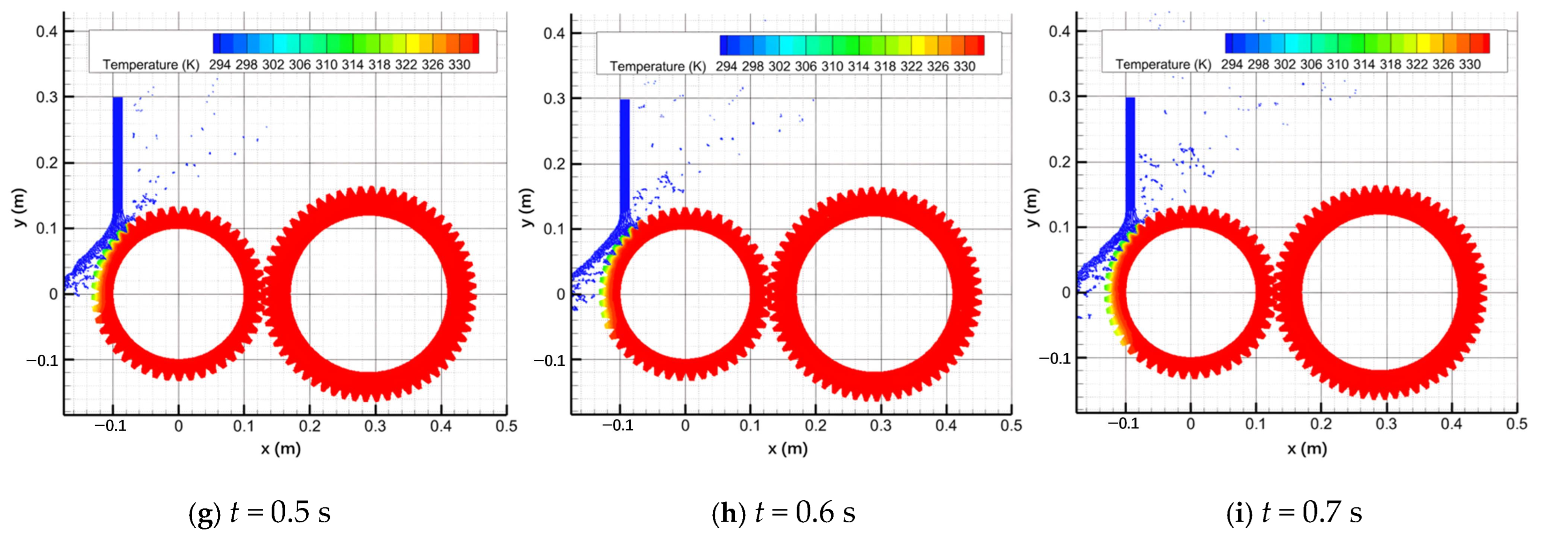
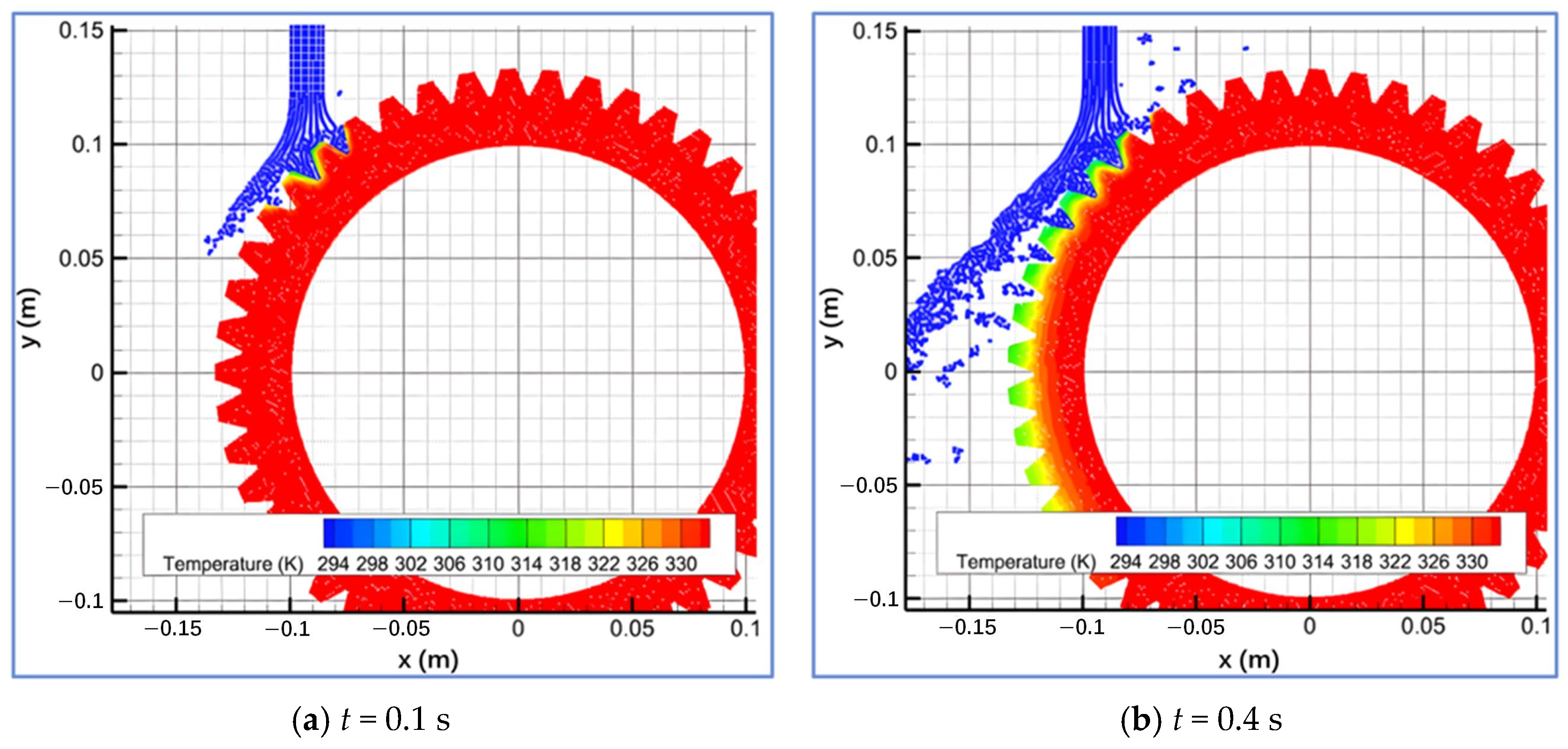
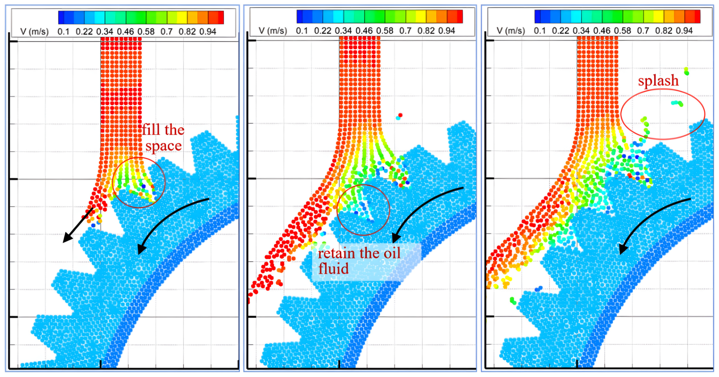
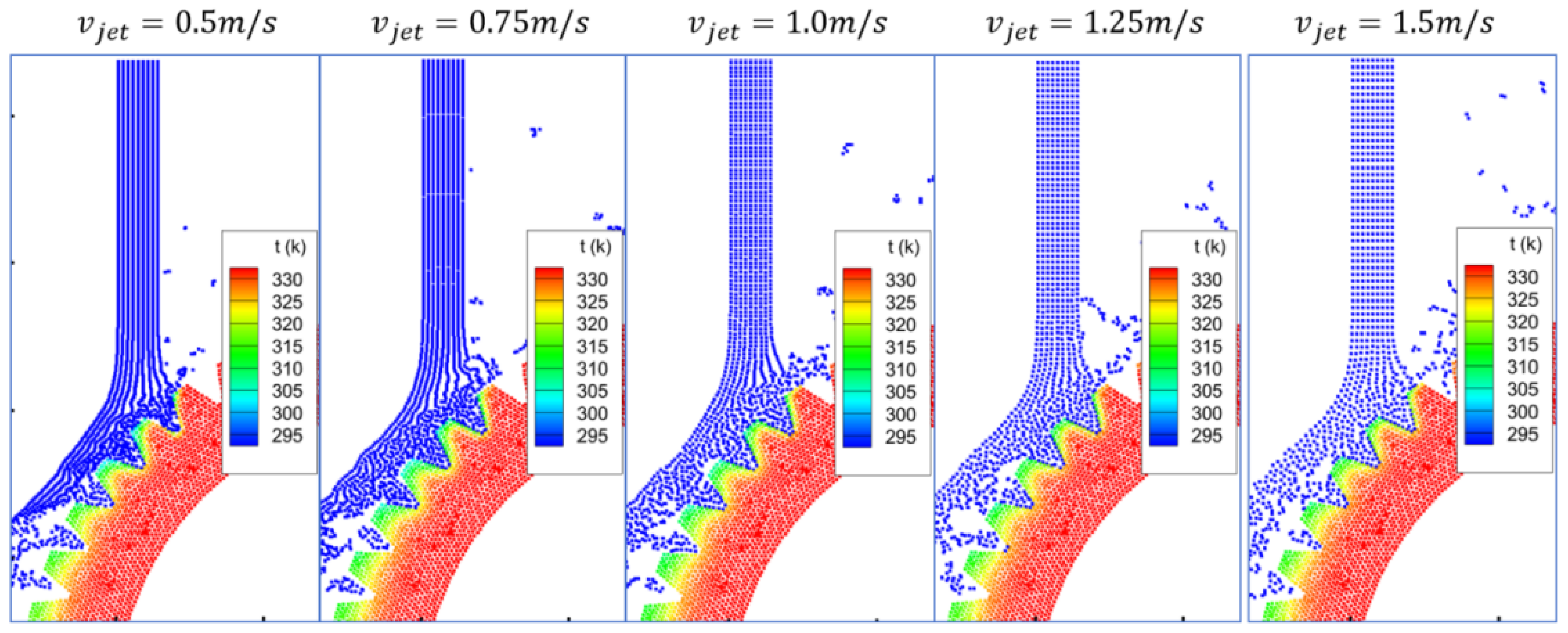
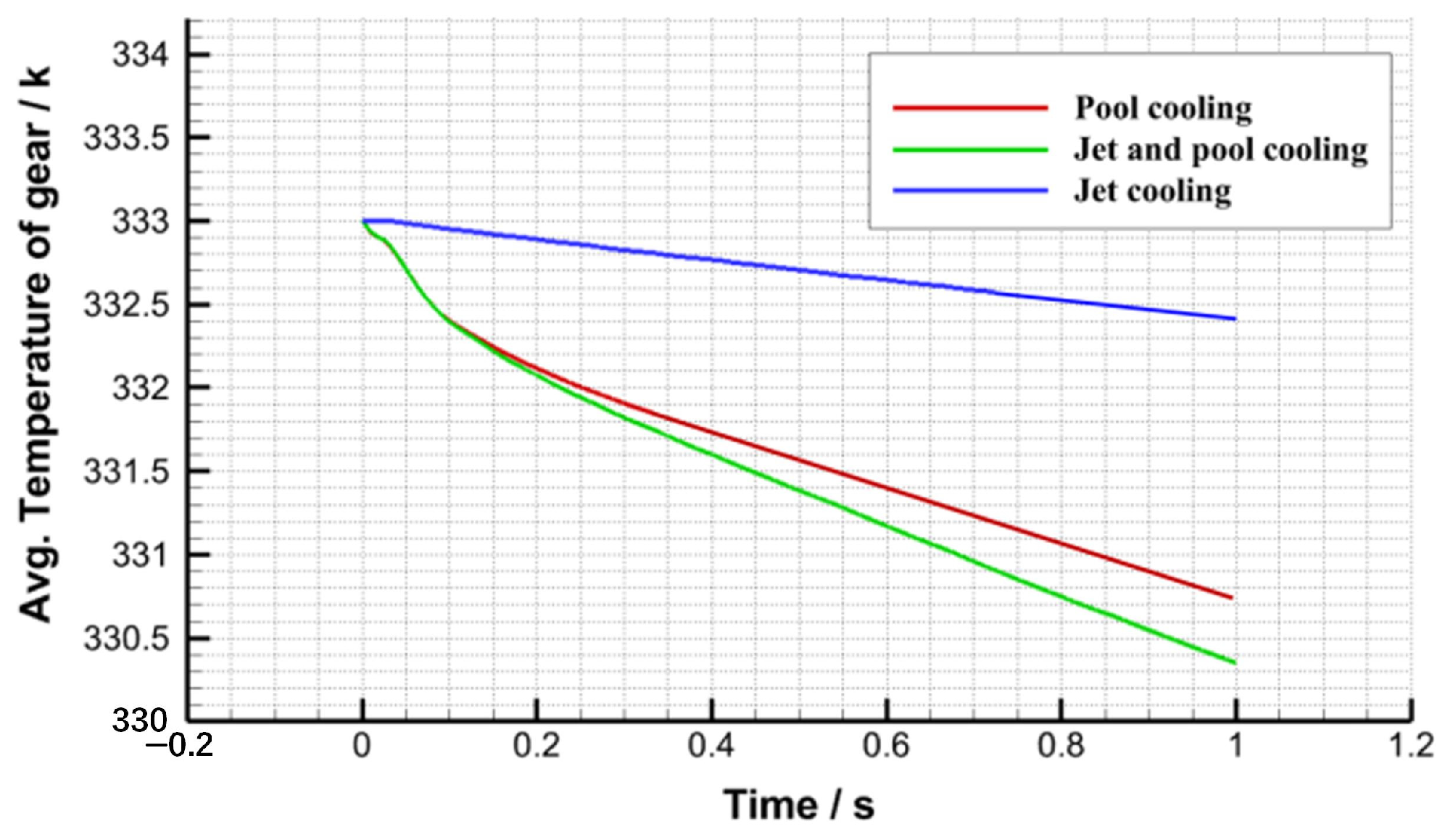
4.2. Results of Transmission Gear Oil Jet Cooling

This subsection simulates the gear cooling process under the action of jet oil cooling. As shown in the figure, a jet oil column is set above the left side of the small gear, with a width of 15 mm and a length of 160 mm. An inlet boundary condition is set at the top of the jet oil column to simulate a continuous jet process. A total of five jet velocities were simulated, which are 0.5 m/s, 0.75 m/s, 1.0 m/s, 1.25 m/s, and 1.5 m/s. The physical properties of the oil are set the same as in the previous subsection. The time step is set to 0.00001 s, and the total number of particles is 30,000. At the initial moment, the jet fluid does not contact the gears; after the calculation begins, the jet fluid moves towards the gears at the set initial velocity, while both gears start to rotate.

Figure 8 displays the simulated temperature distribution results at different moments during the process of jet impact lubrication of the gears. As shown in the figure, at the initial moment, the jet impacts the gears with an initial velocity of 1.0 m/s; at 0.1 s, the jet oil column comes into contact with the tooth surface of the small gear, and as the small gear rotates counterclockwise, the lubricating oil fills the two tooth spaces; due to the counterclockwise rotation of the gear tooth spaces, the jet is deflected to the lower left, and a certain splash effect is produced in the upper right. At 0.15 s, the lubricating oil gradually fills the third tooth space; at 0.3 s and 0.4 s, the lubricating oil respectively fills four and five tooth spaces; under the subsequent impact of the jet, it is basically possible to ensure that there is lubricating oil in five tooth spaces. It can also be seen from the figure that in the gear area that has been sprayed by the jet, the temperature has significantly decreased; while the tooth root interior still shows a higher temperature, close to the initial temperature. The animation of the simulation results of the gear rotation and jet oil cooling process can be found in the Supplementary File.

Figure 9 provides an enlarged view of the local area impacted by the jet, from which the overall temperature distribution on the gear surface during the spraying process can be seen. Due to the use of continuous jet cooling, as the gear rotates, the cooling effect on the gear surface tooth area is essentially uniform along the circumference of the gear. Figure 10 shows the process from the jet contacting the tooth surface, filling the tooth surface, to leaving the tooth surface. The black arrows in Figure 10 represent the direction of gear rotation. Above the tooth surface in the direction opposite to the jet, the splash effect of the fluid is also observed.

Figure 11 presents the simulation results under different oil jet velocities. As shown in Figure 12a, there is a trend that the cooling speed of the gears increases with the increase of the jet velocity. The higher the jet velocity, the faster the cooling speed of the gears. However, after the jet velocity exceeds 1.0 m/s, the trend of the gear cooling speed change is no longer significant, indicating that there is an optimal jet velocity to achieve a balance between oil consumption and cooling speed. Figure 12b provides the variation curves of the average temperature of the gears over time at different gear-rotation speeds. In this case, the jet velocity is fixed at 1.0 m/s. As shown in the figure, as the gear-rotation speed increases, the rate of temperature decrease of the gears also gradually increases; the rate of temperature decrease of the gears represents the cooling rate, and the results show that the cooling rate of the gears is essentially linearly related to the gear-rotation speed. In actual gear lubrication and cooling processes, the rotation speed of the gears generally depends on the driving device or the size of the load. An increase in rotation speed enhances the contact efficiency between the gears and the oil, which can improve the cooling effect to some extent.

Figure 13 presents the simulation results of the gear-cooling process under the combined action of oil jet and oil pool cooling. As shown in the figure, under the joint action of oil jet and oil pool, both the large gear and the small gear are effectively cooled; within the simulated time range, 3/4 of the circumference of the small gear’s teeth show obvious cooling effects. The simulation results indicate that the fluid–solid–thermal coupling model established in this paper is capable of simulating the rotation of gears, the fluid–solid coupling of oil jet and oil pool fluids, and the heat-transfer process, demonstrating good computational stability and efficiency for this complex issue.

Figure 14 also compares the temperature-change curves of the average gear temperature over time under three cooling methods. It can be seen from the figure that oilpool cooling is a more effective cooling method compared to oil jet cooling. However, oil jet cooling can achieve localized spot cooling, which can address the cooling of areas that cannot be effectively cooled by oil pool cooling. For example, in the rocker arm of a coal mining machine (as illustrated in Figure 15), in addition to the motion between multiple gears in the transmission system, there is also the swinging of the rocker arm, and the oil in the rocker arm is a typical liquid sloshing problem, which further increases the difficulty of simulating this issue. From the simulation results of this paper, it can be seen that the meshless SPH model established in this paper has great potential for simulating the complex processes of gear operation and oil pool sloshing in the rocker arm of a coal mining machine.

5. Summary

This paper successfully constructs a fluid–solid–thermal coupling model based on the mesh-free SPH method to simulate the interaction between gear meshing rotation and lubricating fluids. The model effectively handles fluid–solid coupling issues during gear rotation, while also considering the heat transfer processes. This provides a new perspective for understanding gear lubrication and cooling. The simulation results reveal that oil pool cooling is more effective for overall temperature reduction due to its uniform cooling effect across gear surfaces. However, oil jet cooling offers localized cooling benefits, which can be particularly useful for cooling specific areas not effectively reached by oil pool cooling, such as in complex machinery like the rocker arm of a coal mining machine. Combining both cooling methods enhances cooling efficiency, leveraging the strengths of each to provide both overall and localized cooling effects, which is especially beneficial in complex mechanical systems.

The model demonstrates excellent computational stability and efficiency, accurately simulating gear rotation, fluid–solid interactions, and heat transfer processes. This makes it a powerful tool for analyzing complex mechanical and fluid dynamics problems. The meshless SPH model used in this study shows significant potential for simulating complex processes, such as the operation of gears and oil pool sloshing in machinery like the rocker arm of a coal mining machine, highlighting its applicability in various engineering applications where traditional modeling techniques may be limited. Future work can further improve the model by considering factors such as the thermal expansion characteristics of the oil and the variation of viscosity with temperature, which would enhance its accuracy and applicability. Additionally, exploring the potential application of this model in practical engineering problems, such as those encountered in coal mining machinery, offers promising avenues for further research and development.

References

1. Burberi, E.; Fondelli, T.; Andreini, A.; Facchini, B.; Cipolla, L. CFD simulations of a meshing gear pair. In Proceedings of the ASME Turbo Expo 2016: Turbomachinery Technical Conference and Exposition, New York, NY, USA, 13 June 2016; p. V05AT15A024. [Google Scholar] [CrossRef]
2. Ouyang, T.; Mo, X.; Lu, Y.; Wang, J. CFD-vibration coupled model for predicting cavitation in gear transmissions. Int. J. Mech. Sci. 2022, 225, 107377. [Google Scholar] [CrossRef]
3. Marchesse, Y.; Changenet, C.; Ville, F.; Velex, P. Investigations on CFD simulations for predicting windage power losses in spur gears. J. Mech. Des. 2011, 133, 024501. [Google Scholar] [CrossRef]
4. Keller, M.C.; Kromer, C.; Cordes, L.; Schwitzke, C.; Bauer, H.J. CFD study of oil-jet gear interaction flow phenomena in spur gears. Aeronaut. J. 2020, 124, 1301–1317. [Google Scholar] [CrossRef]
5. Hildebrand, L.; Dangl, F.; Paschold, C.; Lohner, T.; Stahl, K. Cfd analysis on the heat dissipation of a dry-lubricated gear stage. Appl. Sci. 2022, 12, 10386. [Google Scholar] [CrossRef]
6. Strasser, W. CFD investigation of gear pump mixing using deforming/agglomerating mesh. J. Fluids Eng. 2007, 129, 476–484. [Google Scholar] [CrossRef]
7. Mastrone, M.N.; Concli, F. CFD simulations of gearboxes: Implementation of a mesh clustering algorithm for efficient simulations of complex system’s architectures. Int. J. Mech. Mater. Eng. 2021, 16, 12. [Google Scholar] [CrossRef]
8. Tan, Y.; Ni, Y.; Wu, J.; Li, L.; Tan, D. Machinability evolution of gas–liquid-solid three-phase rotary abrasive flow finishing. Int. J. Adv. Manuf. Technol. 2024, 131, 2145–2164. [Google Scholar] [CrossRef]
9. Mastrone, M.N.; Concli, F. A multi domain modeling approach for the CFD simulation of multi-stage gearboxes. Energies 2022, 15, 837. [Google Scholar] [CrossRef]
10. Felter, C.L.; Walther, J.H.; Henriksen, C. Moving least squares simulation of free surface flows. Comput. Fluids 2014, 91, 47–56. [Google Scholar] [CrossRef]
11. Spandan, V.; Lohse, D.; de Tullio, M.D.; Verzicco, R. A fast moving least squares approximation with adaptive Lagrangian mesh refinement for large scale immersed boundary simulations. J. Comput. Phys. 2018, 375, 228–239. [Google Scholar] [CrossRef]
12. Hu, M.; Tan, Q.; Feng, D.; Ren, Y.; Huang, Y. Simulation of rock crack propagation and failure behavior based on a mixed failure model with SPH. Rock Mech. Rock Eng. 2024, 57, 9575–9596. [Google Scholar] [CrossRef]
13. Feng, D.; Yi, C.; Hu, M.; Gao, T.; Huang, Y. Simulation of non-cohesive soil turning based on an SPH model. Comput. Geotech. 2023, 160, 105502. [Google Scholar] [CrossRef]
14. Dong, X.; Hao, G.; Yu, R. Two-dimensional smoothed particle hydrodynamics (SPH) simulation of multiphase melting flows and associated interface behavior. Eng. Appl. Comp. Fluid Mech. 2022, 16, 588–629. [Google Scholar] [CrossRef]
15. Dong, X.; Zhang, Q.; Liu, Y.; Liu, X. Improved mesh-free SPH approach for loose top coal caving modeling. Particuology 2024, 95, 1–27. [Google Scholar] [CrossRef]
16. Hu, W.; Chen, Z. A multi-mesh MPM for simulating the meshing process of spur gears. Comput. Struct. 2003, 81, 1991–2002. [Google Scholar] [CrossRef]
17. Lei, Z.; Wu, B.; Wu, S.; Nie, Y.; Cheng, S.; Zhang, C. A material point-finite element (MPM-FEM) model for simulating three-dimensional soil-structure interactions with the hybrid contact method. Comput. Geotech. 2022, 152, 105009. [Google Scholar] [CrossRef]
18. Dong, X.; Feng, L.; Zhang, Q. Droplet asymmetry bouncing on structured surfaces: A simulation based on SPH method. Int. J. Adhes. Adhes. 2024, 132, 103734. [Google Scholar] [CrossRef]
19. Dong, X.; Hao, G.; Liu, Y. Efficient mesh-free modeling of liquid droplet impact on elastic surfaces. Eng. Comput. 2023, 39, 3441–3471. [Google Scholar] [CrossRef]
20. Huang, C.; Hu, C.; An, Y.; Shi, C.; Feng, C.; Wang, H.; Liu, Q.; Wang, X. Numerical simulation of the large-scale Huangtian (China) landslide-generated impulse waves by a GPU-accelerated three-dimensional soil–water coupled SPH model. Water Resour. Res. 2023, 59, e2022WR034157. [Google Scholar] [CrossRef]
21. Imin, R.; Geni, M. Stress analysis of gear meshing impact based on SPH method. Math. Probl. Eng. 2014, 2014, 328216. [Google Scholar] [CrossRef]
22. Ji, Z.; Stanic, M.; Hartono, E.A.; Chernoray, V. Numerical simulations of oil flow inside a gearbox by Smoothed Particle Hydrodynamics (SPH) method. Tribol. Int. 2018, 127, 47–58. [Google Scholar] [CrossRef]
23. Keller, M.C.; Braun, S.; Wieth, L.; Chaussonnet, G.; Dauch, T.F.; Koch, R.; Schwitzke, C.; Bauer, H.J. Smoothed particle hydrodynamics simulation of oil-jet gear interaction. J. Tribol. 2019, 141, 071703. [Google Scholar] [CrossRef]
24. Groenenboom, P.; Cartwright, B.; McGuckin, D.; Amoignon, O.; Mettichi, M.Z.; Gargouri, Y.; Kamoulakos, A. Numerical studies and industrial applications of the hybrid SPH-FE method. Comput. Fluids 2019, 184, 40–63. [Google Scholar] [CrossRef]
25. Sun, P.N.; Pilloton, C.; Antuono, M.; Colagrossi, A. Inclusion of an acoustic damper term in weakly-compressible SPH models. J. Comput. Phys. 2023, 483, 112056. [Google Scholar] [CrossRef]
26. Guan, X.S.; Sun, P.N.; Xu, Y.; Lyu, H.G.; Geng, L.M. Numerical studies of complex fluid-solid interactions with a six degrees of freedom quaternion-based solver in the SPH framework. Ocean Eng. 2024, 291, 116484. [Google Scholar] [CrossRef]
27. Guo, C.; Zhang, H.; Qian, Z.; Liu, M. Smoothed-interface SPH model for multiphase fluid-structure interaction. J. Comput. Phys. 2024, 518, 113336. [Google Scholar] [CrossRef]
28. Ma, Y.; Zhou, X.; Zhang, F.; Weißenfels, C.; Liu, M. A novel smoothed particle hydrodynamics method for multi-physics simulation of laser powder bed fusion. Comput. Mech. 2024, 74, 1009–1036. [Google Scholar] [CrossRef]
29. Guo, X.; Yang, M.; Li, F.; Zhu, Z.; Cui, B. Investigation on cryogenic cavitation characteristics of an inducer considering thermodynamic effects. Energies 2024, 17, 3627. [Google Scholar] [CrossRef]
30. Zheng, B.X.; Cai, Z.W.; Zhao, P.D.; Xu, X.Y.; Chan, T.S.; Yu, P. A generalized density dissipation for weakly compressible smoothed particle hydrodynamics. Phys. Fluids 2024, 36, 083325. [Google Scholar] [CrossRef]
31. Becker, M.; Teschner, M. Weakly compressible SPH for free surface flows. In Proceedings of the 2007 ACM SIGGRAPH/Eurographics Symposium on Computer Animation, San Diego, CA, USA, 2 August 2007; p. 209. [Google Scholar] [CrossRef]
32. Antuono, M.; Colagrossi, A.; Marrone, S. Numerical diffusive terms in weakly-compressible SPH schemes. Comput. Phys. Commun. 2012, 183, 2570–2580. [Google Scholar] [CrossRef]
33. Cleary, P.W.; Monaghan, J.J. Conduction modelling using smoothed particle hydrodynamics. J. Comput. Phys. 1999, 148, 227–264. [Google Scholar] [CrossRef]
34. Liu, M.B.; Liu, G. Smoothed particle hydrodynamics (SPH): An overview and recent developments. Arch. Comput. Method Eng. 2010, 17, 25–76. [Google Scholar] [CrossRef]
Figure 1. SPH model for gear meshing with fluid–solid coupling.
Processes 13 00730 g001
Figure 2. Numerical flow chart.
Processes 13 00730 g002
Figure 3. FORTRAN code structure.
Processes 13 00730 g003
Figure 4. Simulation results of the gear rotation and oil pool cooling process.
Processes 13 00730 g004
Figure 5. Simulation results of the evolution process of the fluid surface between the gears.
Processes 13 00730 g005
Figure 6. Fluid behavior after the gear enters the liquid surface.
Processes 13 00730 g006
Figure 7. Simulation results of fluid splash behavior between gears at different rotation speeds.
Processes 13 00730 g007
Figure 8. Simulation results of gear rotation and jet oil cooling process (jet velocity 1.0 m/s).
Processes 13 00730 g008aProcesses 13 00730 g008b
Figure 9. Simulation results of gear temperature distribution during the early and late stages of oil jet cooling.
Processes 13 00730 g009
Figure 10. Simulation results of the transient process of jet impact on rotating gears.
Processes 13 00730 g010
Figure 11. Simulation results of temperature fields at different oil jet velocities.
Processes 13 00730 g011
Figure 12. Curve of the average temperature of the gear changing over time.
Processes 13 00730 g012
Figure 13. Simulation results of combined oil jet and oil pool cooling.
Processes 13 00730 g013aProcesses 13 00730 g013b
Figure 14. Curves of the average temperature of the gear over time under three cooling methods.
Processes 13 00730 g014
Figure 15. Schematic diagram of the coal mining machine rocker arm structure and swinging position.
Processes 13 00730 g015
Disclaimer/Publisher’s Note: The statements, opinions and data contained in all publications are solely those of the individual author(s) and contributor(s) and not of MDPI and/or the editor(s). MDPI and/or the editor(s) disclaim responsibility for any injury to people or property resulting from any ideas, methods, instructions or products referred to in the content.