
Tuning of PID Controllers Using Reinforcement Learning for Nonlinear System Control


Abstract
:1. Introduction
- -
- -
- In the aerospace industry, PID controllers are used to control the flight of aircraft. They can help to keep the aircraft straight and on course, even in difficult conditions [3].
- -
- In the automotive industry, PID controllers are used to control the engine, transmission, and other systems. They can help to improve vehicles’ performance, efficiency, and safety [4].
2. Twin Delayed Deep Deterministic Policy Gradient (TD3) Algorithm
2.1. Basics of Reinforcement Learning Algorithms
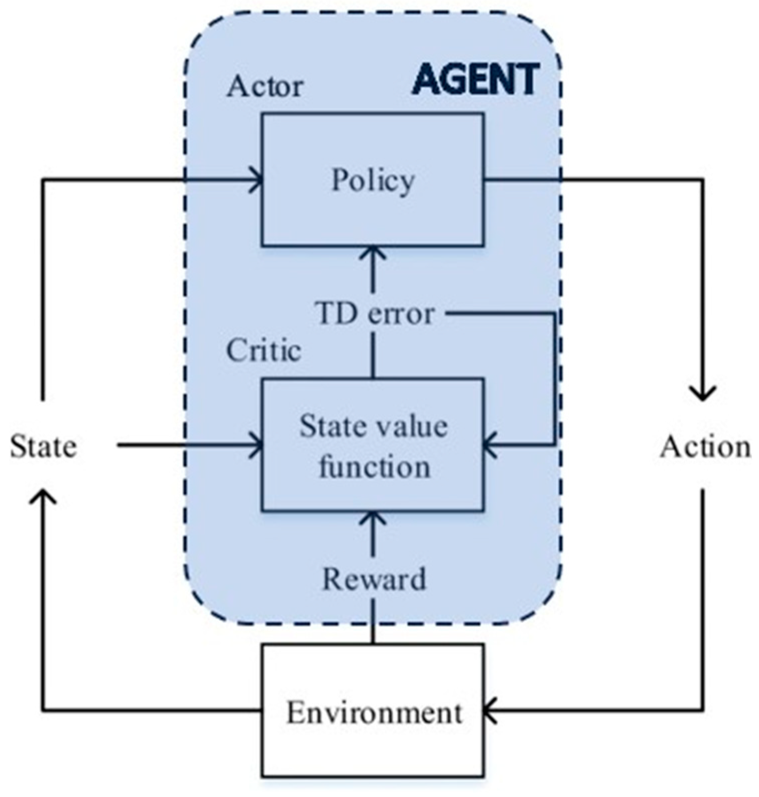
- Agent: The agent is the entity that is learning to behave in an environment. The most common structure for the agent is composed of two elements: the critic and actor. The critic estimates the expected cumulative reward (value) associated with being in a certain state and following the policy defined by the actor. The actor is responsible for learning and deciding on the optimal policy—the mapping from states to actions. It is essentially the decision-maker or policy function.
- Environment: The environment is the world that the agent interacts with.
- State: The state is the current condition of the environment.
- Action: An action is something that the agent can do in the environment.
- Reward: A reward is a signal that indicates whether an action was good or bad.
- Policy: A policy is a rule that tells the agent which action to take in a given state.
- Value function: A value function is a measure of how beneficial it is to be in a given state.
2.2. Deep Deterministic Policy Gradient
- —TD error;
- —learning rate.
- Initialize the critic and actor networks;
- Collect data from the environment and store them in the replay buffer;
- Sample a batch of experiences from the replay buffer;
- Compute the target Q-value using the target networks and update the critic using the mean-squared Bellman error loss;
- Update the actor policy using the sampled batch, aiming to maximize the estimated Q-value;
- Periodically update the target networks with a soft update;
- Repeat steps 3–6 until the desired performance is achieved.
2.3. TD3—The Main Characteristics
| Algorithm 1. TD3 | |
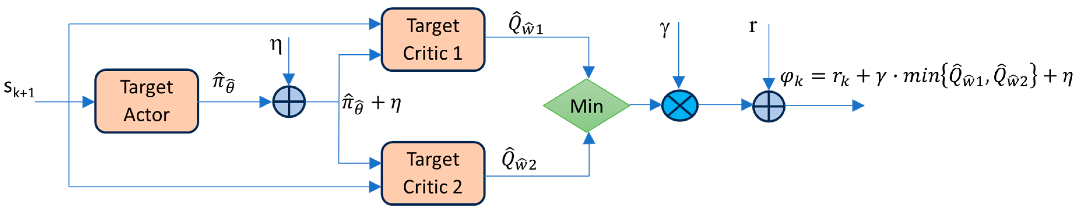
| 1. Initialize critic networks , and actor network with random parameters , , . 2. Initialize the parameters of the target networks: , , 3. Initialize replay buffer B for k= 1 to T do 4. Select action with exploration noise and observe reward rk and new state sk+1 5. Store transition (sk, ak, sk+1, rk) in B 6. Sample mini-batch of N transitions (sk, ak, sk+1, rk) from B and compute | |
| | (14) |
| 7. Update critic parameters: | |
| (15) | |
| 8. Update θ by the deterministic policy gradient | |
| (16) | |
| 9. Update target networks: | |
|
| (17) |
| end for | |
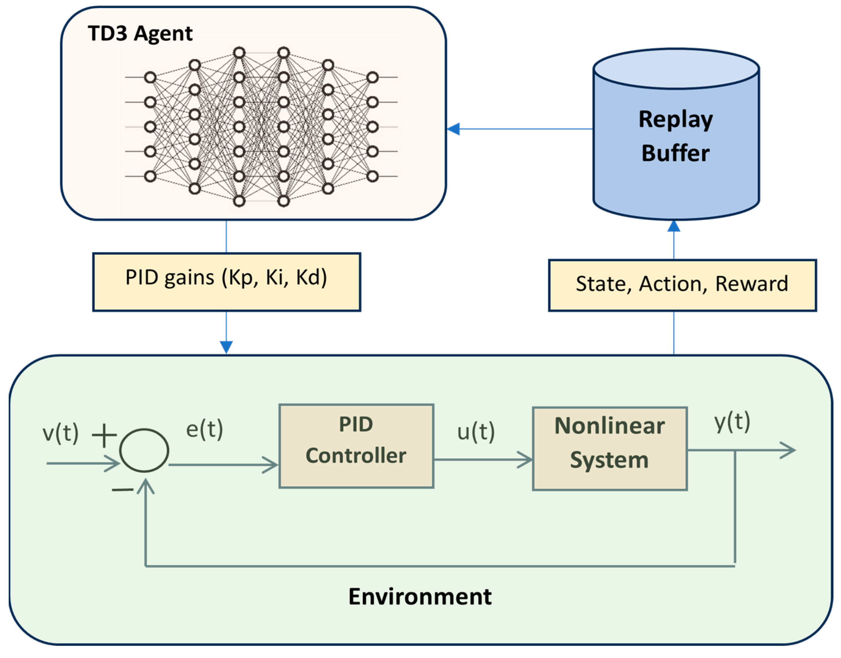
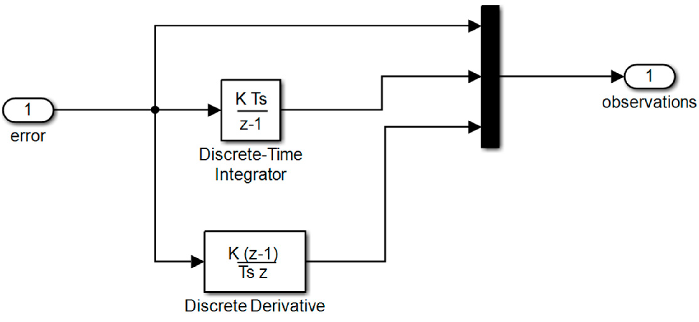
3. Tunning of PID Controllers Using TD3 Algorithm
- u is the output of the actor neural network;
- Kp, Ki, and Kd are the PID controller parameters;
- e(t) = v(t) − y(t), where e(t) is the system error, y(t) is the system output, and v(t) is the reference signal.
4. Tuning PID Controller for Biotechnological System—Classical Approach
4.1. Linearization of a Biotechnological System
- represents the state vector (the concentrations of the system’s variables);
- denotes the vector of the reaction kinetics (the rates of the reactions);
- is the matrix of the yield coefficients;
- represents the rate of production;
- is the exchange between the bioreactor and the exterior.
4.2. Ziegler–Nichols Method
4.3. Pole Placement Method
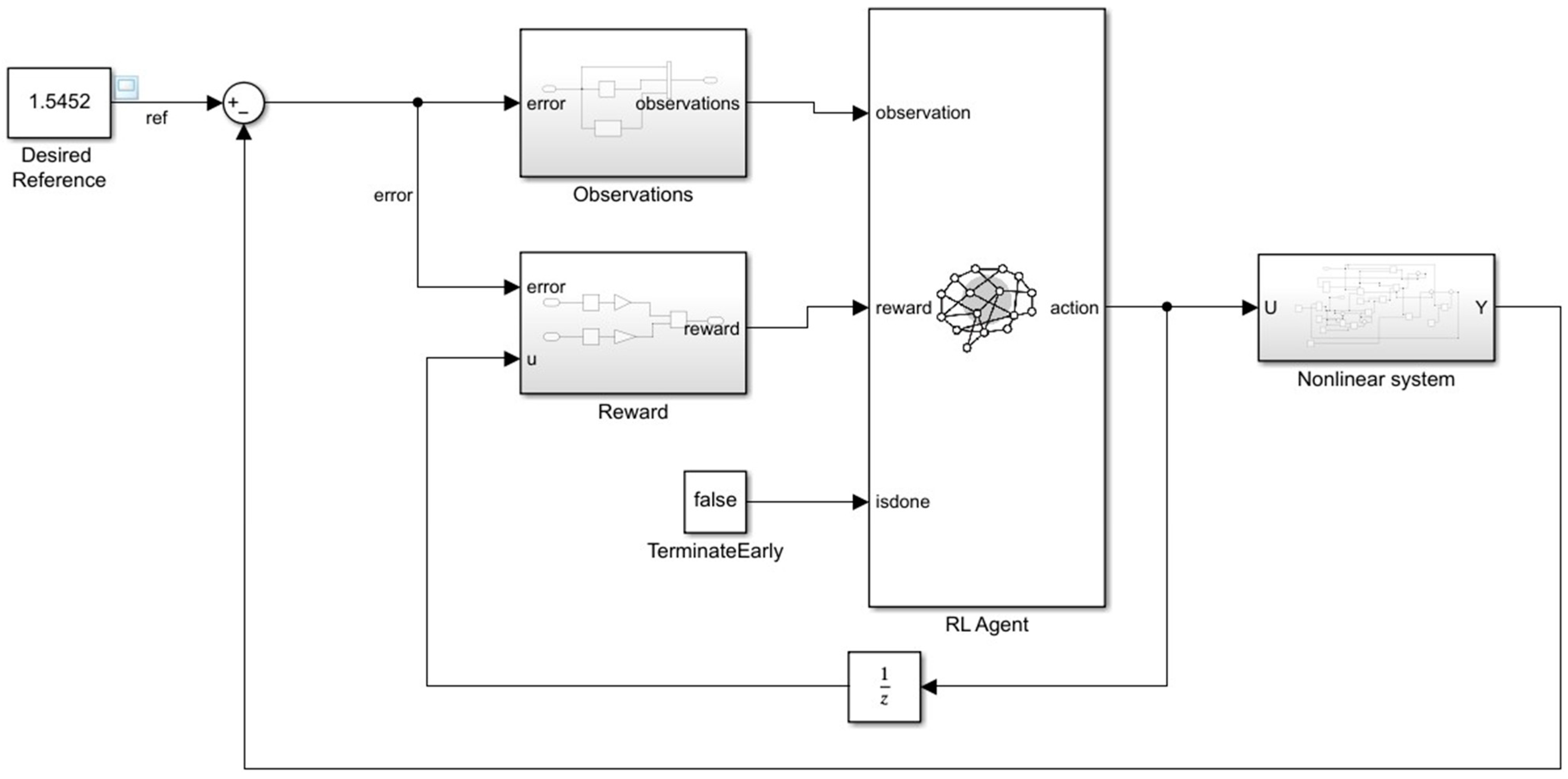
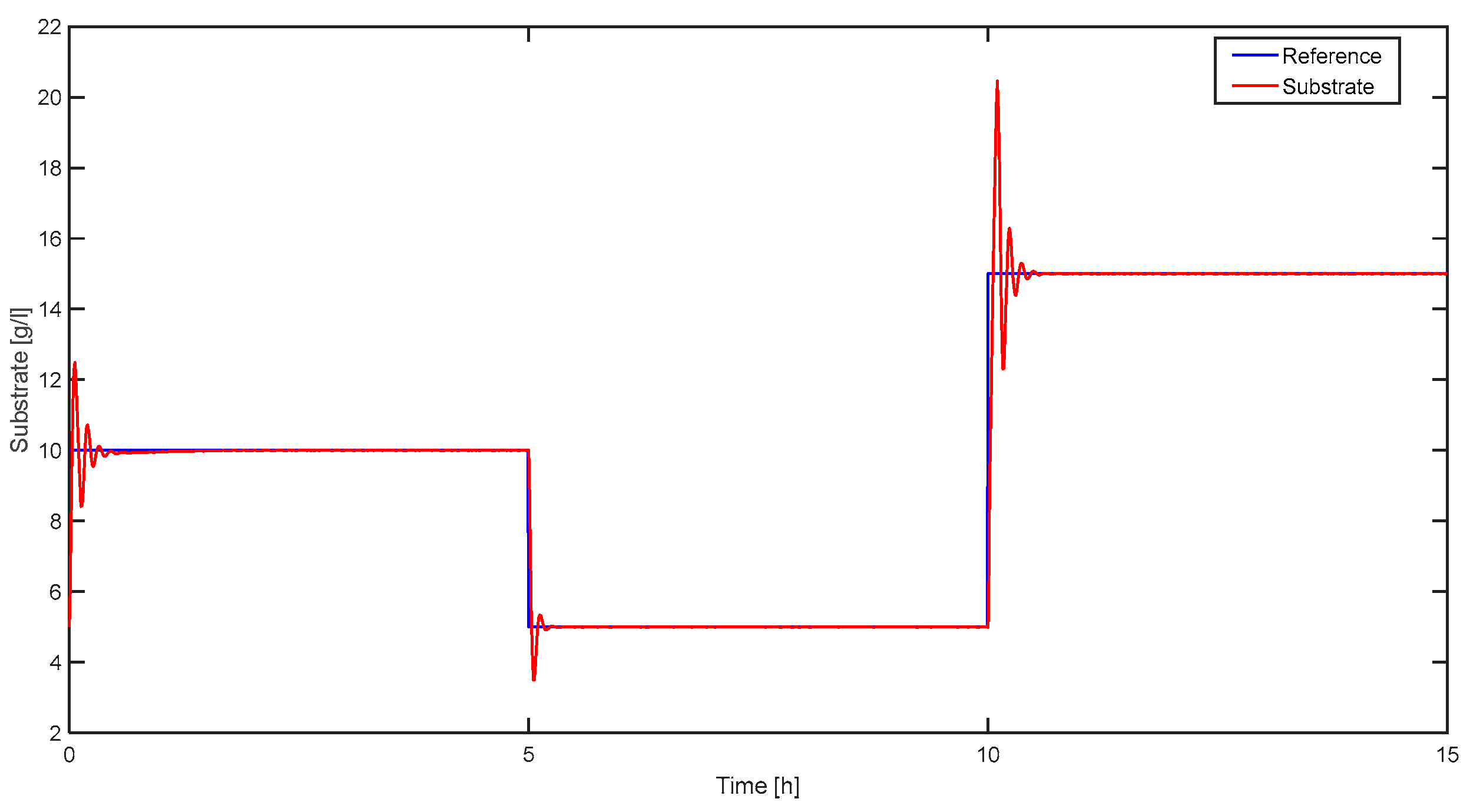
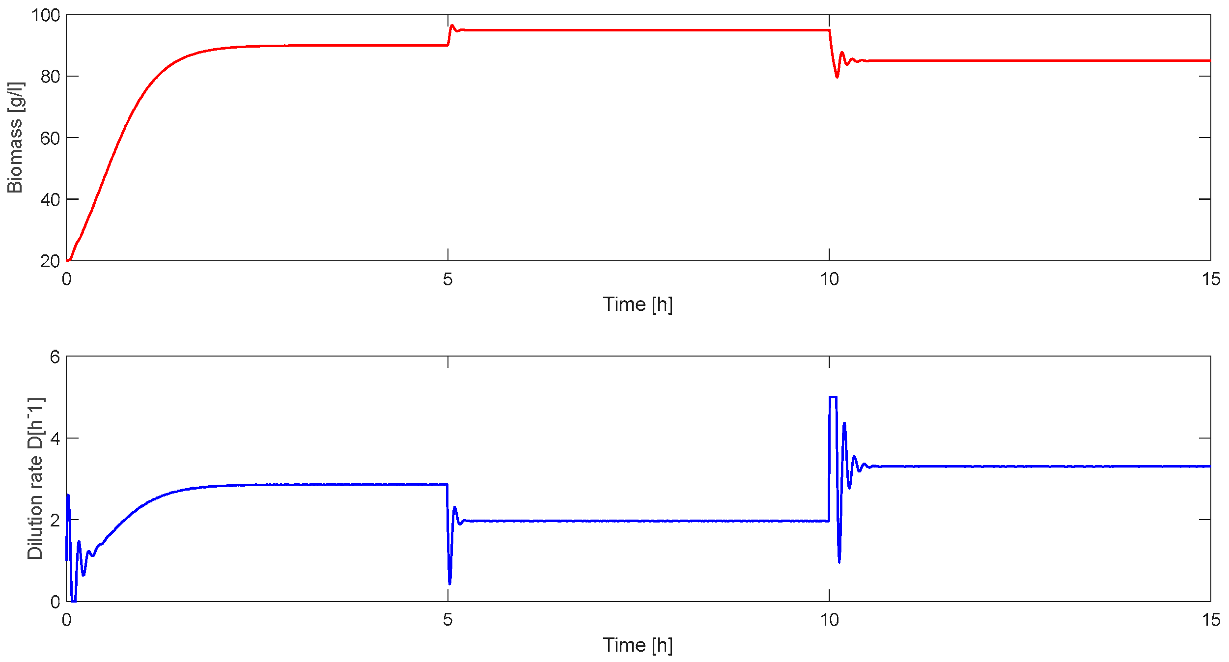
5. Simulation Results
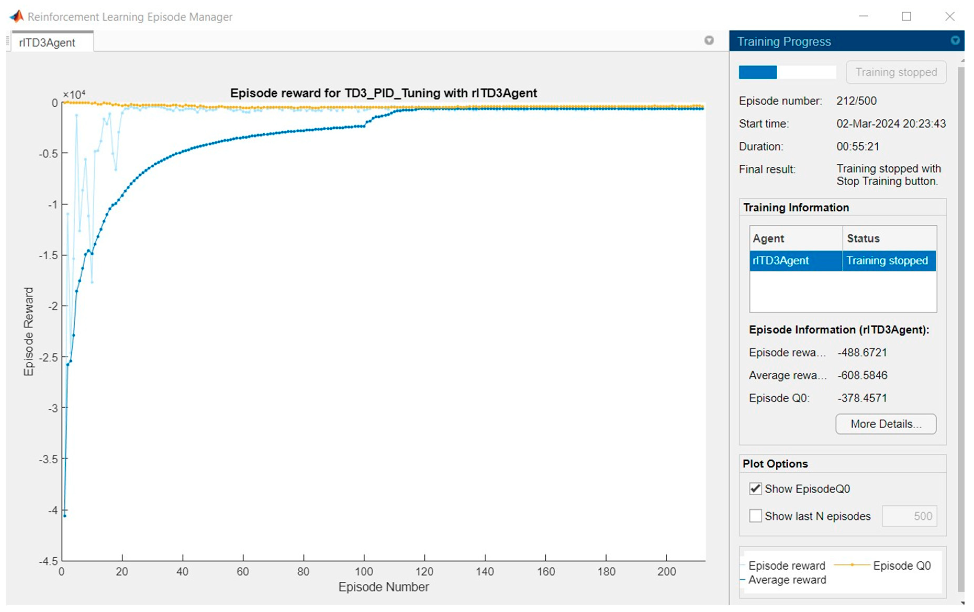
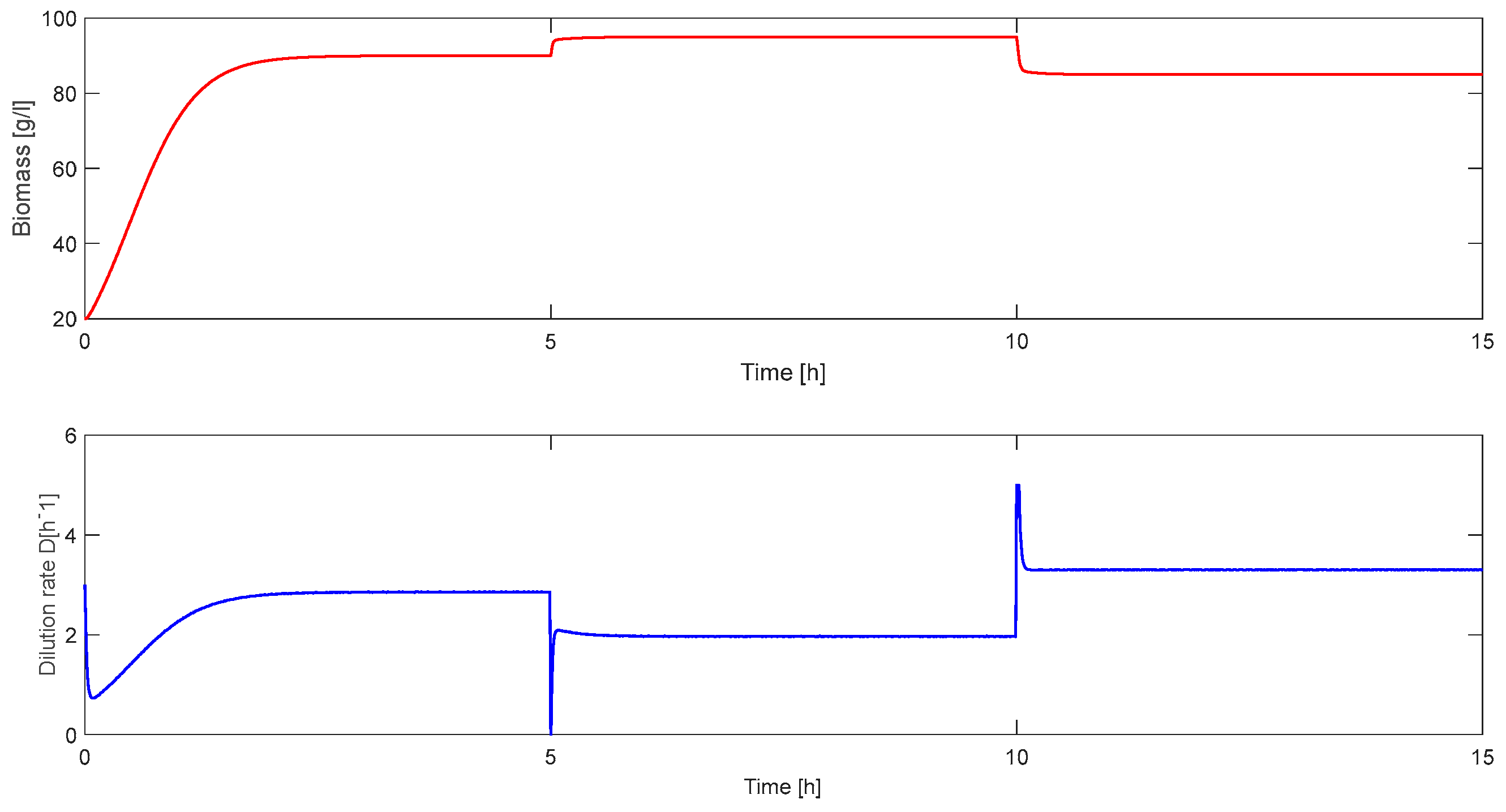
5.1. RL Approach
5.2. Classical Approach
6. Conclusions
Author Contributions
Funding
Data Availability Statement
Conflicts of Interest
Abbreviations
| PID | Proportional–Integral–Derivative |
| TD3 | Twin Delayed Deep Deterministic Policy Gradient |
| FOPTD | First-Order Plus Time Delay |
| RL | Reinforcement Learning |
| AI | Artificial Intelligence |
| SARSA | State–Action–Reward–State–Action |
| DQN | Deep Q-Network |
| DDPG | Deep Deterministic Policy Gradient |
| TRPO | Trust Region Policy Optimization |
References
- Borase, R.P.; Maghade, D.; Sondkar, S.; Pawar, S. A review of PID control, tuning methods and applications. Int. J. Dyn. Control. 2021, 9, 818–827. [Google Scholar] [CrossRef]
- Bucz, Š.; Kozáková, A. Advanced methods of PID controller tuning for specified performance. In PID Control for Industrial Processes; BoD–Books on Demand: Norderstedt, Germany, 2018; pp. 73–119. [Google Scholar]
- Noordin, A.; Mohd Basri, M.A.; Mohamed, Z. Real-Time Implementation of an Adaptive PID Controller for the Quadrotor MAV Embedded Flight Control System. Aerospace 2023, 10, 59. [Google Scholar] [CrossRef]
- Amanda Danielle, O.S.D.; André Felipe, O.A.D.; João Tiago, L.S.C.; Domingos, L.A.N.; Carlos Eduardo, T.D. PID Control for Electric Vehicles Subject to Control and Speed Signal Constraints. J. Control. Sci. Eng. 2018, 2018, 6259049. [Google Scholar] [CrossRef]
- Aström, K.J.; Hägglund, T. Advanced PID Control; ISA-The Instrumentation, Systems, and Automation Society: Research Triangle Park, NC, USA, 2006; Volume 461. [Google Scholar]
- Liu, G.; Daley, S. Optimal-tuning PID control for industrial systems. Control Eng. Pract. 2001, 9, 1185–1194. [Google Scholar] [CrossRef]
- Aström, K.J.; Hägglund, T. Revisiting the Ziegler–Nichols step response method for PID control. J. Process Control. 2004, 14, 635–650. [Google Scholar] [CrossRef]
- Lee, H.G. Linearization of Nonlinear Control Systems; Springer: Singapore, 2022. [Google Scholar]
- Wilson, J.; Rugh, J.; Shamma, S. Research on gain scheduling. Automatica 2000, 36, 1401–1425. [Google Scholar] [CrossRef]
- Ge, Z.; Liu, F.; Meng, L. Adaptive PID Control for Second Order Nonlinear Systems. In Proceedings of the Chinese Control And Decision Conference (CCDC), Hefei, China, 22–24 August 2020; pp. 2926–2931. [Google Scholar] [CrossRef]
- Lillicrap, T.P.; Hunt, J.; Pritzel, A.; Heess, N.; Erez, T.; Tassa, Y. Continuous control with deep reinforcement learning. arXiv 2015, arXiv:150902971. [Google Scholar]
- Brunton, S.L.; Kutz, J.N. Data-Driven Science and Engineering: Machine Learning, Dynamical Systems, and Control; Cambridge University Press: Cambridge, UK, 2019. [Google Scholar]
- Shi, H.; Zhang, L.; Pan, D.; Wang, G. Deep Reinforcement Learning-Based Process Control in Biodiesel Production. Processes 2024, 12, 2885. [Google Scholar] [CrossRef]
- Chowdhury, M.A.; Al-Wahaibi, S.S.S.; Lu, Q. Entropy-maximizing TD3-based reinforcement learning for adaptive PID control of dynamical systems. Comput. Chem. Eng. 2023, 178, 108393. [Google Scholar] [CrossRef]
- Yin, F.; Yuan, X.; Ma, Z.; Xu, X. Vector Control of PMSM Using TD3 Reinforcement Learning Algorithm. Algorithms 2023, 16, 404. [Google Scholar] [CrossRef]
- Liu, R.; Cui, Z.; Lian, Y.; Li, K.; Liao, C.; Su, X. AUV Adaptive PID Control Method Based on Deep Reinforcement Learning. In Proceedings of the China Automation Congress (CAC), Chongqing, China, 17–19 November 2023; pp. 2098–2103. [Google Scholar] [CrossRef]
- Kofinas, P.; Dounis, A.I. Fuzzy Q-Learning Agent for Online Tuning of PID Controller for DC Motor Speed Control. Algorithms 2018, 11, 148. [Google Scholar] [CrossRef]
- Massenio, P.R.; Naso, D.; Lewis, F.L.; Davoudi, A. Assistive Power Buffer Control via Adaptive Dynamic Programming. IEEE Trans. Energy Convers. 2020, 35, 1534–1546. [Google Scholar] [CrossRef]
- Zhao, J. Adaptive Dynamic Programming and Optimal Control of Unknown Multiplayer Systems Based on Game Theory. IEEE Access 2022, 10, 77695–77706. [Google Scholar] [CrossRef]
- El-Sousy, F.F.M.; Amin, M.M.; Al-Durra, A. Adaptive Optimal Tracking Control Via Actor-Critic-Identifier Based Adaptive Dynamic Programming for Permanent-Magnet Synchronous Motor Drive System. IEEE Trans. Ind. Appl. 2021, 57, 6577–6591. [Google Scholar] [CrossRef]
- Massenio, P.R.; Rizzello, G.; Naso, D. Fuzzy Adaptive Dynamic Programming Minimum Energy Control of Dielectric Elastomer Actuators. In Proceedings of the IEEE International Conference on Fuzzy Systems (FUZZ-IEEE), New Orleans, LA, USA, 23–26 June 2019; pp. 1–6. [Google Scholar] [CrossRef]
- Fujimoto, S.; Hoof, H.; Meger, D. Addressing function approximation error in actor-critic methods. In Proceedings of the 35th International Conference on Machine Learning, Stockholm, Sweden, 10–15 July 2018; pp. 1587–1596. [Google Scholar]
- Muktiadji, R.F.; Ramli, M.A.M.; Milyani, A.H. Twin-Delayed Deep Deterministic Policy Gradient Algorithm to Control a Boost Converter in a DC Microgrid. Electronics 2024, 13, 433. [Google Scholar] [CrossRef]
- Sutton, R.S.; Barto, A.G. Reinforcement Learning: An Introduction; MIT Press: Cambridge, MA, USA, 2018. [Google Scholar]
- Yao, J.; Ge, Z. Path-Tracking Control Strategy of Unmanned Vehicle Based on DDPG Algorithm. Sensors 2022, 22, 7881. [Google Scholar] [CrossRef] [PubMed]
- Hasselt, H.V.; Guez, A.; Silver, D. Deep reinforcement learning with double Q-learning. In Proceedings of the AAAAI Conference on Artificial Intelligence, Phoenix, AZ, USA, 12–17 February 2016; Volume 30, pp. 1–7. [Google Scholar]
- Rathore, A.S.; Mishra, S.; Nikita, S.; Priyanka, P. Bioprocess Control: Current Progress and Future Perspectives. Life 2021, 11, 557. [Google Scholar] [CrossRef] [PubMed]
- Roman, M.; Selişteanu, D. Modeling of microbial growth bioprocesses: Equilibria and stability analysis. Int. J. Biomath. 2016, 9, 1650067. [Google Scholar] [CrossRef]
- Sendrescu, D.; Petre, E.; Selisteanu, D. Nonlinear PID controller for a Bacterial Growth Bioprocess. In Proceedings of the 2017 18th International Carpathian Control Conference (ICCC), Sinaia, Romania, 28–31 May 2017; Institute of Electrical and Electronics Engineers (IEEE): Piscataway, NJ, USA, 2017; pp. 151–155. [Google Scholar]
- MathWorks—Twin-Delayed Deep Deterministic Policy Gradient Reinforcement Learning Agent. Available online: https://www.mathworks.com/help/reinforcement-learning/ug/td3-agents.html (accessed on 20 February 2025).


| Notation | RL Element |
|---|---|
| sk | current state |
| sk+1 | next state |
| ak | current action |
| ak+1 | next action |
| rk | reward at state sk |
| Q | Q-function (critic) |
| π | policy function (actor) |
| δ | TD target |
| action space | |
| state space |
| Parameter | Value |
|---|---|
| Mini-batch size | 128 |
| Experience buffer length | 500,000 |
| Gaussian noise variance | 0.1 |
| Steps in episode | 200 |
| Maximum number of episodes | 1000 |
| Optimizer | Adam |
| Discount factor | 0.97 |
| Fully connected learning size | 32 |
| Critic learning rate | 0.01 |
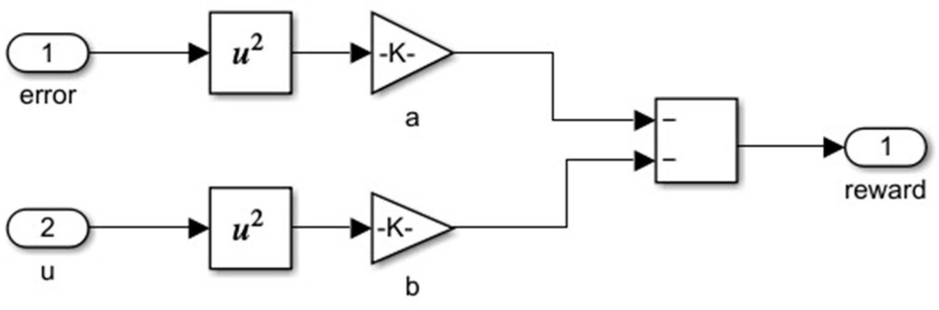
| Reward function | a = 0.1, b = 0.02 |
| Actor learning rate | 0.01 |
| Tuning Method | Kp | Ki | Kd | Overshoot [%] | Settling Time [h] |
|---|---|---|---|---|---|
| TD3-based tuning | 0.62 | 3.57 | 0.00023 | 0 | 0.8 |
| PID Tuner app from Matlab | 0.207 | 28.64 | 0.00037 | 20–40% | 0.4–0.5 |
| Ziegler–Nichols tuning | 1.76 | 11.36 | 0.00054 | 35–45% | 0.5–0.6 |
| Pole placement tuning | 1.32 | 14.27 | 0.00043 | 10–22% | 0.5–0.55 |
Disclaimer/Publisher’s Note: The statements, opinions and data contained in all publications are solely those of the individual author(s) and contributor(s) and not of MDPI and/or the editor(s). MDPI and/or the editor(s) disclaim responsibility for any injury to people or property resulting from any ideas, methods, instructions or products referred to in the content. |
© 2025 by the authors. Licensee MDPI, Basel, Switzerland. This article is an open access article distributed under the terms and conditions of the Creative Commons Attribution (CC BY) license (https://creativecommons.org/licenses/by/4.0/).
Share and Cite
Bujgoi, G.; Sendrescu, D. Tuning of PID Controllers Using Reinforcement Learning for Nonlinear System Control. Processes 2025, 13, 735. https://doi.org/10.3390/pr13030735
Bujgoi G, Sendrescu D. Tuning of PID Controllers Using Reinforcement Learning for Nonlinear System Control. Processes. 2025; 13(3):735. https://doi.org/10.3390/pr13030735
Chicago/Turabian StyleBujgoi, Gheorghe, and Dorin Sendrescu. 2025. "Tuning of PID Controllers Using Reinforcement Learning for Nonlinear System Control" Processes 13, no. 3: 735. https://doi.org/10.3390/pr13030735
APA StyleBujgoi, G., & Sendrescu, D. (2025). Tuning of PID Controllers Using Reinforcement Learning for Nonlinear System Control. Processes, 13(3), 735. https://doi.org/10.3390/pr13030735