A New Bayesian Inversion Method for Thixotropic Model Parameters of Waxy Crude Oil

Abstract

Waxy crude oil displays complex rheological behaviors, including viscoelasticity, thixotropy, and yield stress, under the gelling point temperature. To characterize these complex rheological behaviors, numerous models have been proposed, all of which typically involve extensive unknown parameters to be determined. Traditional least squares methods for determining model parameters have problems such as difficulty in determining the initial values for parameter fitting, susceptibility to falling into local optimal solutions, and instability of the fitting results. For this purpose, this paper proposes a parameter inversion method for determining thixotropic model parameters by integrating Adaptive Differential Evolution (ADE) with Bayesian inversion. By leveraging the global search capability of the ADE algorithm and the probabilistic uncertainty quantification advantages of the Bayesian method, the accuracy and stability of model parameter fitting are significantly enhanced. This paper conducted a comparative analysis between the proposed thixotropic model parameter inversion method and traditional methods based on the Houska model, using the thixotropic test data of Daqing and Xianhe waxy crude oil. The results show that the fitting errors of the new method are significantly smaller than those of the least squares method. Furthermore, the new method can invert to obtain superior thixotropic model parameters even under suboptimal initial parameter conditions while maintaining robust optimization capability. The novel method for inverting thixotropic model parameters outperforms the least squares method in terms of algorithm convergence, stability, robustness, and model fitting accuracy, solving the problem of difficult fitting of unknown parameters in thixotropic models.

1. Introduction

Above the wax precipitation point temperature, wax in waxy crude oil is entirely dissolved in the liquid crude oil. At the wax precipitation point, wax begins to crystallize and form small wax particles suspended in the liquid crude oil. As the temperature further decreases, the formed wax crystal particles interconnect to create a three-dimensional sponge-like network structure, resulting in the gelation of the crude oil [1,2,3,4]. Near the pour point temperature, waxy crude oil exhibits complex rheological behaviors such as viscoelasticity, thixotropy, and yield stress [5,6]. Over the past few decades, numerous scholars have conducted extensive research on the thixotropic properties of waxy crude oil and have developed several thixotropic models. Among these, the models of structural dynamic type have the best applicability to waxy crude oil.

Based on the treatment of the viscoelastic behavior of materials before and near the yield point, thixotropic models can be broadly categorized into two types: viscoplastic thixotropic models and viscoelastic–thixotropic models. To date, several representative viscoplastic models have been reported in the literature, such as the Houska model [7] and the Guo model [8]. These models do not account for the viscoelastic phase where shear stress increases with strain before reaching the yield point, but they characterize the yield behavior through yield stress. In contrast, viscoelastic–thixotropic models incorporate the viscoelastic response of materials before the yield point, with typical examples including the Dullaert model [9], Zhu model [10], and Geest model [11].

Thixotropic models typically contain a large number of unknown parameters. There are two common types of parameter regression methods for thixotropic models: one type is based on optimization methods such as least squares, the conjugate gradient method [12], and neural networks to solve nonlinear equations and determine all model parameters at once; the other type determines model parameters stepwise in groups (first try to obtain some individual parameters of the model from experiments, and, then, determine the remaining parameters using the least squares method for fitting). The stepwise parameter determination method may exacerbate experimental errors and compromise the fitting performance.

To address the issue of model initial values, Yuan [13] proposed using an Adaptive Differential Evolution (ADE) algorithm to obtain initial model values. This algorithm is less affected by the initial values of parameter iterations, improving fitting performance. In this study, three regression strategies were proposed and compared. It was found that the combination of stepwise regression and overall regression outperforms either overall regression or stepwise regression alone, as the latter may compromise the accuracy of the experimental results. Building on this, Yuan [14] proposed a multi-objective regression strategy and an Adaptive Non-dominated Sorting Differential Evolution (Adaptive NSDE) algorithm, enhancing model fitting accuracy. However, although ADE can improve search performance to some extent, it may still face convergence issues or fail to fit in cases of excessively large parameter spaces or unclear boundaries, leading to optimization instability.

Traditional least squares methods for determining model parameters have two main limitations. First, they require initial values for the unknown parameters during the fitting process. However, since these initial values are unsuspected, the selection of initial values for iteration is highly subjective and uncertain. Second, the strong nonlinearity among model parameters often restricts traditional least-squares-based methods to local optimal solutions. Consequently, the fitting results are highly sensitive to initial values. Different initial values may lead to convergence towards different model parameters, thereby introducing a degree of uncertainty into the fitting results and ultimately degrading the fitting performance.

In recent years, Bayesian inversion has achieved widespread success in uncertainty modeling and parameter optimization, as it is applied to parameter estimation in complex systems such as geophysics, medical imaging reconstruction, and material science [15,16]. Wang [17] highlighted the advantages of Bayesian methods in the rheological fitting of complex fluids (e.g., polymer solutions, colloids), particularly in avoiding local optima and improving fitting accuracy. The strength of Bayesian inversion lies in its ability to integrate prior information with experimental data, iteratively updating posterior distributions during parameter optimization, thereby enhancing fitting robustness. Compared to least squares, Bayesian methods can account for uncertainty in parameter estimation, avoid local optima, and maintain high fitting accuracy even under significant initial value perturbations [18,19].

To address the challenges of determining initial parameter values, avoiding local optima, and achieving stable results in model parameter fitting, this study proposes a new approach for determining the parameters of the thixotropic model, which combines the Bayesian inversion with the Adaptive Differential Evolution (ADE) algorithm. The ADE algorithm is employed to resolve the issue of providing initial parameter values [20,21], while the Bayesian inversion is used to mitigate the problem of converging to local optima. The effectiveness of the proposed method is validated through comparative analysis with traditional methods using thixotropic experimental data from Daqing and Xianhe waxy crude oils. The results demonstrate that the newly proposed parameter inversion method is capable of significantly enhancing the fitting accuracy of the thixotropic model under conditions where the initial values of the model parameters are suboptimal or the model parameter range is broad. Moreover, it can yield more robust parameters for the thixotropic model.

2. Thixotropic Models and Experimental Data

To verify the feasibility of the proposed thixotropic model parameter inversion method, which integrates ADE into Bayesian inversion, the representative Houska thixotropic model was selected to fit the thixotropic test data. The thixotropic test experiment includes stepwise increases in shear rate tests and hysteresis loop tests of Daqing and Xianhe waxy crude oils.

2.1. Thixotropic Models

The Houska model is one of the most renowned constitutive models in the field of rheology, frequently employed to characterize the rheological behavior of waxy crude oil. It integrates the relationship between yield stress and the shear rate, effectively describing the viscoelastic behavior of materials under varying shear rates. The model comprises a rheological constitutive equation and a kinetic equation, as shown in Equations (1) and (2). The first kinetic equation includes terms for structure buildup and breakdown, where λ represents the structural parameter of the material. This thixotropic model incorporates eight parameters: ${\tau }_{\mathrm{y}0}$, ${\tau }_{\mathrm{y}1}$, $K$, $\mathsf{\Delta }K$, $n$, $a$, $b$, and $m$.

$$\tau =\left({\tau }_{\mathrm{y}0}+\lambda {\tau }_{\mathrm{y}1}\right)+\left(K+\lambda \mathsf{\Delta }K\right){\dot{\gamma }}^n$$

(1)

$${\displaystyle \frac{\mathrm{d}\lambda }{\mathrm{d}t}}=a\left(1-\lambda \right)-\mathrm{b}\lambda {\dot{\gamma }}^m$$

(2)

In the equation, $\tau$ represents the shear stress, describing the response of the fluid under external shear forces; ${\tau }_{\mathrm{y}0}$ denotes the static yield stress (intrinsic yield stress), indicating the yield stress of the fluid in the absence of structural reconstruction; ${\tau }_{\mathrm{y}1}$ represents the structure-dependent additional yield stress, characterizing the contribution of structuralization to the yield stress; $K$ is the consistency coefficient (viscosity factor), describing the viscosity characteristics of the material; $\mathsf{\Delta }K$ is the structure-dependent additional consistency coefficient, reflecting the influence of structuralization on consistency; $n$ is the rheological behavior index, describing the shear-thinning or shear-thickening behavior of non-Newtonian fluids; $a$ is the structure recovery rate coefficient, representing the material’s self-recovery capability under external shear forces; $b$ is the structure breakdown rate coefficient, indicating the intensity of the shear-induced structural breakdown; and $m$ is the breakdown index, controlling the extent to which the shear rate influences structural breakdown.

2.2. Experimental Data

To conduct thixotropic model fitting analysis, stepwise increases in shear rate test data and hysteresis loop tests data of Daqing and Xianhe waxy crude oils were used.

For Daqing waxy crude oil, the experimental data were sourced from a reference focused on thixotropic testing [22]. The experiments were performed using a HAAKE MARS III controlled-stress rheometer equipped with a Z41Ti coaxial cylinder measuring system, which was manufactured by Thermo Fisher SCIENTIFIC in Germany.

The rheological experiments on Daqing crude oil (pour point 32 °C) were carried out at temperatures of 32 °C, 33 °C, 34 °C, and 35 °C. Shear step tests were conducted at rates of 1 s⁻¹, 2 s⁻¹, 4 s⁻¹, 8 s⁻¹, 16 s⁻¹, 32 s⁻¹, and 64 s⁻¹, each maintained for 450 s. In hysteresis loop tests, the shear rate linearly increased from 0 to 50 s⁻¹ over 200 s then decreased back to 0 s⁻¹ over the same time, repeated twice. Each measurement was taken with a new oil sample.

As for Xianhe waxy crude oil, the experimental data were derived from conducted experiments. The setup included a HAAKE MARS60 controlled-stress rheometer with a CC41/Ti coaxial cylinder measuring system, which was manufactured by Thermo Fisher SCIENTIFIC in Germany. The rheological experiments on Xianhe crude oil (pour point 34 °C) were performed at 34 °C, 35 °C, 36 °C, and 37 °C. For the shear step tests, shear rates of 1 s⁻¹, 2 s⁻¹, 4 s⁻¹, 8 s⁻¹, 16 s⁻¹, 32 s⁻¹, 64 s⁻¹, and 128 s⁻¹ were employed, with each rate maintained for 1200 s. In the hysteresis loop tests, the shear rate was linearly ramped up from 0 s⁻¹ to 50 s⁻¹ over 200 s and then linearly ramped down to 0 s⁻¹ over the same duration, and this cycle was performed twice. Each measurement utilized a fresh oil sample.

3. A New Inversion Method for Thixotropic Model Parameters

To address the issues of high initial value sensitivity and the tendency to fall into local optima in model parameter optimization, this study proposes a novel strategy for determining model parameters by integrating Adaptive Differential Evolution (ADE) with Bayesian inversion. Initially, the ADE algorithm was employed for global exploration to obtain reasonable initial parameter estimates. Subsequently, these initial values were refined locally using either Bayesian inversion. The ADE algorithm facilitates efficient global optimization across a broad parameter space through adaptive mutation and crossover operations, thereby significantly reducing the sensitivity to initial value selection. Meanwhile, the Bayesian inversion method dynamically updates the posterior distribution of parameters by integrating prior information with experimental data, effectively avoiding local optima and markedly enhancing the accuracy and stability of the fit.

3.1. ADE-Based Bayesian Inversion Method

The Adaptive Differential Evolution (ADE) algorithm was utilized to conduct a global search, offering more reasonable initial parameter values. Subsequently, Bayesian inversion was applied for local optimization. This integrated approach significantly improves the accuracy and stability of thixotropic model fitting. This approach not only mitigates the issue of sensitivity to initial values but also optimizes parameter selection across a broader range, improving the applicability and accuracy of the thixotropic model.

(1)

Initial Parameter Estimation Using ADE Algorithm

The fundamental concept of the Adaptive Differential Evolution (ADE) algorithm revolves around maintaining a population of individuals and generating new generations through operations such as mutation, crossover, and selection, progressively approaching the optimal solution to the problem. Each individual represents a potential solution, and the algorithm employs adaptive strategies to enhance convergence speed and precision. The workflow of the algorithm can be divided into four key steps: mutation, crossover, selection, and iteration, which can be summarized as follows:

① Mutation: A random perturbation is applied to each individual in the population $x_i^g$:

$$F=\left\{\begin{array}{c}{F}_a+\mathrm{rand}\left(0,1\right)\times F_b,\hspace{1em}\mathrm{if} \mathrm{rand}\left(0,1\right)<{\eta }_1\\ F_{i,\mathrm{G}},\hspace{1em}\hspace{1em}\hspace{1em}\hspace{1em}\hspace{1em}\hspace{1em}\hspace{1em}\mathrm{otherwise}\end{array}\right.$$

(3)

$$v_i^{\mathrm{G}+1}=x_r^{\mathrm{G}}+F\cdot \left(x_s^{\mathrm{G}}-x_t^{\mathrm{G}}\right)$$

(4)

In the equation, $v$ represents the mutation vector; $x_r^{\mathrm{G}}$, $x_s^{\mathrm{G}}$, $x_t^{\mathrm{G}}$ are randomly selected individuals from the population, where $r$, $s$, and $t$ are distinct random indices within the range [1, NP]. These indices must be mutually exclusive and differ from the index $i$. $F$ denotes the scaling factor, while $F_a$, $F_b$, and ${\eta }_1$ are control parameters for $F$. NP represents the population size, and $\mathrm{G}$ signifies the generation number.

It is noteworthy that the mutation variables may exceed their predefined bounds during the mutation process. In this study, lower and upper bounds will be imposed on the mutation variables to ensure that they remain within the permissible range.

② Crossover: The trial individual $v_i^{\mathrm{G}+1}$ undergoes binomial crossover to ensure that at least one parameter is altered:

$$CR=\left\{\begin{array}{c}\mathrm{rand}\left(0,1\right),\hspace{1em}\mathrm{if} \mathrm{rand}\left(0,1\right)<{\eta }_2\\ C_{i,\mathrm{G}},\hspace{1em}\hspace{1em}\hspace{1em} \mathrm{otherwise}\end{array}\right.$$

(5)

$$u_i^{\mathrm{G}+1}=\left\{\begin{array}{c}{v}_i^{\mathrm{G}+1},\mathrm{if} \mathrm{rand}\left(0,1\right)<CR \mathrm{or} j=j_{\mathrm{rand}}\\ x_i^{\mathrm{G}},\hspace{0.17em}\hspace{0.17em}\mathrm{otherwise}\end{array}\right.$$

(6)

In the equation, $CR$ represents the crossover probability; $j_{\mathrm{rand}}$ is a randomly selected index within the range [1, D], where D denotes the dimensionality of the vector. This ensures that at least one variable in each individual is derived from the mutation. Additionally, ${\eta }_2$ serves as the control parameter for $CR$.

③ Selection: Individuals with superior fitness are selected for the next generation based on the fitness function $J\left(x\right)$:

$$x_i^{\mathrm{G}+1}=\left\{\begin{array}{c}{u}_i^{\mathrm{G}+1},J\left(u_i^{\mathrm{G}+1}\right)<J\left(x_i^{\mathrm{G}}\right)\\ x_i^{\mathrm{G}},\hspace{1em}\mathrm{otherwise}\end{array}\right.$$

(7)

④ Iteration: The variables of all individuals in the G-th generation are updated by those in the (G + 1)-th generation. This process is repeated, encompassing mutation, crossover, and selection, until the predefined maximum number of generations is reached.

(2)

Bayesian Parameter Inversion

The parameters obtained through the Adaptive Differential Evolution (ADE) algorithm are further optimized using the Bayesian inversion method. The specific process is as follows: First, the ADE algorithm was employed to explore the global optimal solution, generating multiple candidate solutions within the population through mutation, crossover, and selection operations, from which a suitable initial parameter set was derived. Subsequently, the Bayesian inversion method integrated experimental data with prior distributions, iteratively adjusting parameter values and evaluating the corresponding errors to progressively approach the optimal solution.

The Bayesian inversion method is based on Bayes’ theorem, dynamically adjusting parameter distributions during the optimization process by combining prior distributions with experimental data. It iteratively refines the initial parameter values and evaluates the corresponding model errors to identify the optimal parameters. The core idea is to utilize current error information to guide the search process and gradually enhance the precision of the parameters. The key formula is as follows:

$$P(\theta |D)={\displaystyle \frac{P(D|\theta )P\left(\theta \right)}{P\left(D\right)}}$$

(8)

In the equation, $P(\theta |D)$ represents the posterior distribution of the parameter $\theta$ given the experimental data $D$; $P(D|\theta )$ denotes the likelihood function, which indicates the probability of the data given the parameter $\theta$; $P\left(\theta \right)$ is the prior distribution, representing the initial guess of the parameter $\theta$ in the absence of data; and $P\left(D\right)$ serves as the normalization factor, which is the weighted average of the likelihood functions over all possible parameters.

The Bayesian algorithm consists of initialization, generating parameter samples, evaluating errors, selecting optimal parameters, convergence judgment, and outputting the optimal parameters. The process can be summarized as follows:

① Initialization: The initial parameter $x_0$ is assigned the optimal parameter values obtained from the ADE optimization. An Error Threshold (ET) and a Maximum Permissible Error Count (MPEC) are defined.

② Generating Parameter Samples: Starting from the optimal parameters $x_0$ obtained via ADE, multiple samples $x_s$ are generated by applying random perturbations. These perturbations are based on a normal distribution, as described by the following equation:

$$x_s=x_0+F_S\times \mathrm{randn}\left(1,\mathrm{Length}\left(x_0\right)\right)$$

(9)

In the equation, $F_S$ represents the adjustment factor; $\mathrm{randn}$ denotes the random perturbation following a normal distribution; and $\mathrm{Length}$ is the vector dimensionality function.

③ Evaluating Errors: For each generated sample $x_s$, the predicted shear stress value ${\tau }_{\mathrm{c}}$ is computed using the thixotropic model. This value is then compared with the experimentally obtained shear stress ${\tau }_{\mathrm{e}}$ from thixotropy tests to calculate the error (in this study, the Root Mean Square Error, RMSE, is used).

$$\mathrm{R}\mathrm{M}\mathrm{S}\mathrm{E}=\sqrt{{\displaystyle \frac{1}{N}}\sum _{\mathrm{i}=1}^N{\left[{\tau }_{\mathrm{c}}\left(t\right)-{\tau }_{\mathrm{e}}\left(t\right)\right]}^2}$$

(10)

④ Selecting Optimal Parameters: If the error of a particular sample is smaller than the current optimal error, the current optimal parameter is updated to that sample.

$$x_{\mathrm{Best}}=\min \left(\mathrm{Error}\left(x_s\right)\right)$$

(11)

⑤ Convergence Judgment: The optimization is considered to have converged and is terminated when the error falls below the specified threshold $es$ and remains below it for more than MPEC.

⑥ Outputting Optimal Parameters: When the optimization converges, the final output is the optimal parameter set, which represents the parameters that best fit the given observational data and the model.

(3)

Algorithm Parameter Configuration

In this study, the parameter settings for the Adaptive Differential Evolution (ADE) algorithm were determined by comprehensively considering the optimization convergence speed, search capability, and the need to balance global and local exploration. Based on existing research and multiple experimental comparisons, the following parameters were selected:

① The population size was set to 260, a value determined by the empirical rule of thumb, which typically ranges from 10 to 50 times the parameter dimensionality. This ensures sufficient population diversity even in higher-dimensional optimization problems, thereby mitigating the risk of premature convergence.

② The number of iterations was set to 100, a value determined through experimental tuning to ensure that the algorithm converges to a stable solution with reasonable computational cost while avoiding unnecessary computational overhead.

③ The scaling factor, denoted as F = 0.8, governs the magnitude of variation. It is generally recommended to maintain this value within the range of 0.5 to 1. A value of 0.8 is chosen as it offers a balanced exploratory capability while ensuring convergence stability.

④ The crossover probability factor, denoted as CR = 0.9, plays a pivotal role in expediting convergence. In the context of intricate parameter optimization problems, maintaining CR within the range of 0.8 to 0.9 significantly enhances global search capabilities, thereby circumventing the pitfalls of local optima.

Furthermore, through a series of experimental tests involving various parameter combinations (e.g., F = 0.6, CR = 0.7, etc.), it was observed that the currently selected parameter set achieves an optimal balance between fitting accuracy and convergence efficiency. By integrating global search with local optimization, the aim is to enhance both the precision of model fitting and computational efficiency.

3.2. Least Squares Method

To substantiate the efficacy of the novel approach introduced herein, a comparative analysis was conducted between the proposed method and the least squares method (LSM). LSM optimizes parameters by minimizing the sum of squared errors between experimental data and model predictions. The mathematical formulation of this optimization is expressed as follows:

$$\mathrm{f}(X_{\mathrm{I}})=\sqrt{{\displaystyle \frac{1}{N}}\sum _{\mathrm{q}=1}^N\{({\tau }_{\mathrm{e}}{)}_{\mathrm{q}}-[{\tau }_{\mathrm{c}}(X_{\mathrm{I}}){]}_{\mathrm{q}}{\}}^2}$$

(12)

In the equation, f represents the objective function; $X_{\mathrm{I}}$ denotes the various parameters of the model ($x^1, x^2, x^3, x^4, x^5, x^6, x^7, x^8$), which correspond to (${\tau }_{\mathrm{y}0}$, ${\tau }_{\mathrm{y}1}$, $K$, $\mathsf{\Delta }K$, $n$, $a$, $b$, $m$); $N$ is the total number of experimental data points in the thixotropy test; q is the sequence number of the experimental data in the thixotropy test; ${\tau }_{\mathrm{e}}$ is the shear stress obtained from the thixotropy test; and ${\tau }_{\mathrm{c}}$ is the shear stress derived from the thixotropic model.

4. Results and Discussion

To systematically and comprehensively evaluate the performance of the proposed novel Bayesian inversion methodology for model parameters incorporating Adaptive Differential Evolution (ADE), this study conducts analyses from multiple perspectives:

(1)

The thixotropic test results of Daqing and Xianhe waxy crude oils were utilized to assess the fitting accuracy, computational efficiency, and convergence stability of the proposed parameter inversion method. This evaluation provides quantitative metrics to validate the method’s effectiveness in capturing complex rheological behaviors.

(2)

A series of initial parameter perturbation experiments were conducted to verify the robustness of the proposed inversion methodology. Furthermore, we analyzed the temperature-dependent variations in the fitted model parameters to elucidate their physical significance.

Through multi-faceted comparisons and validations, the applicability and stability of the proposed thixotropic model parameter inversion method are thoroughly investigated, ensuring its reliability across diverse operational conditions and material systems.

4.1. Validation of the New Parameter Inversion Method

4.1.1. Stepwise Increases in Shear Rate Tests

The proposed thixotropic model parameter inversion method (abbreviated as novel method in this paper) and the least squares method (abbreviated as LSM) are, respectively, applied to the Houska model, based on the stepwise increases in shear rate tests for Daqing and Xianhe crude oils. To better compare the fitting effects of the proposed thixotropic model parameter inversion method and the least squares method, the same initial values (not necessarily optimal) are provided for both methods.

The average relative error (MRE) intuitively reflects the relative size of prediction deviations in percentage form, while the Root Mean Square Error (RMSE) highlights model stability by amplifying larger errors. Together, they offer a comprehensive evaluation of prediction accuracy and error distribution characteristics. Their calculation formulas are, respectively, shown in Equations (13) and (14). The Mean Relative Error (MRE) and the Root Mean Square Error (RMSE) of the two methods’ fitting results for the Daqing and Xianhe waxy crude oils are listed in

Table 1. MRE and RMSE of Houska model under stepwise increases in shear rate tests for Daqing crude oil.

T (°C)	RMSE		MRE
	LSM	Novel Method	LSM	Novel Method
32	1.37	0.97	10.48%	8.48%
33	1.04	0.57	17.47%	6.81%
34	2.48	0.33	75.30%	6.18%
35	3.05	0.14	158.64%	4.79%

and

Table 2. MRE and RMSE of Houska model under stepwise increases in shear rate tests for Xianhe crude oil.

T (°C)	RMSE		MRE
	LSM	Novel Method	LSM	Novel Method
34	0.30	0.17	9.37%	3.60%
35	1.10	0.07	91.18%	3.15%
36	1.36	0.04	257.08%	3.41%
37	1.32	0.03	413.31%	3.75%

, respectively.

$$\mathrm{MRE}={\displaystyle \frac{1}{N}}{\displaystyle \sum }_{\mathrm{i}=1}^N\left|{\displaystyle \frac{y_i-\widehat{y_i}}{y_i}}\right|\times 100\%$$

(13)

$$\mathrm{R}\mathrm{M}\mathrm{S}\mathrm{E}=\sqrt{{\displaystyle \frac{1}{N}}\sum _{\mathrm{i}=1}^N{\left[y_i-\widehat{y_i}\right]}^2}$$

(14)

In the formula, N represents the number of data points; $y_i$ is the experimental data value; and $\widehat{y_i}$ represents the calculated data value.

The fitting results in Table 1 were performed under the same set of given initial values, and the fitting results in Table 2 were performed under another set of initial values. As can be seen in Table 1 and Table 2, the proposed thixotropic model parameter inversion method achieves significantly lower fitting errors compared to the least squares method under identical initial conditions. Specifically, the RMSE was reduced by approximately 64.12% and 82.94% for Daqing and Xianhe waxy crude oils, respectively, and the MRE decreased by 67.21% and 88.97%, respectively, on average. Additionally, as temperature varies, the fitting error of least squares method shows considerable fluctuations, whereas the fitting error of proposed thixotropic model parameter inversion method remains essentially unchanged. This highlights the novel method’s effectiveness in adapting to diverse temperature conditions and sustaining robust optimization capabilities. Analysis of the above situation reveals that the least squares method is sensitive to initial values and prone to local optima, whereas the novel method optimizes initial values using ADE, effectively reducing the sensitivity to initial value selection, and employs Bayesian random sampling to avoid local optimum issues. Therefore, the new method offers higher fitting accuracy and stronger adaptability than the least squares method.

In Table 2, it is found that, when the temperature increases from 36 °C to 37 °C, the RMSE and MRE of the two methods show opposite trends. This is because, as the temperature rises, the shear stress values of the waxy crude oil decrease. The same relative error corresponds to a smaller absolute error value, so there is an increase in MRE, while RMSE decreases.

Meanwhile, ADE took an average of 200 s, Bayesian inversion took an average of 15 s, and the least squares method took an average of 10 s, during the computations. However, the computational time of ADE-based Bayesian inversion method remains acceptable, and the inversion accuracy of the new method was significantly enhanced. Consequently, the proposed thixotropic model parameter inversion method demonstrates superior fitting performance compared to the least squares method.

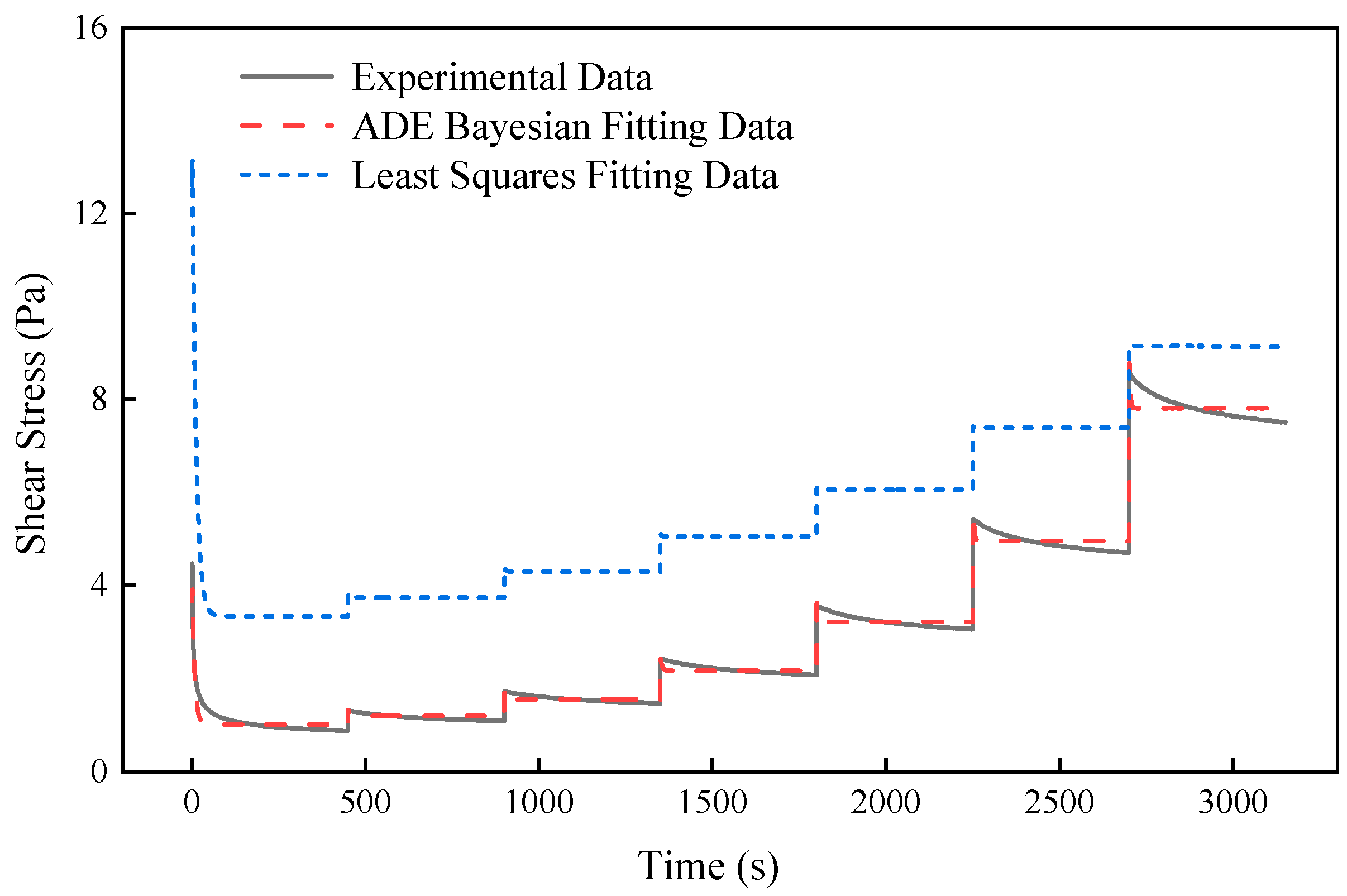
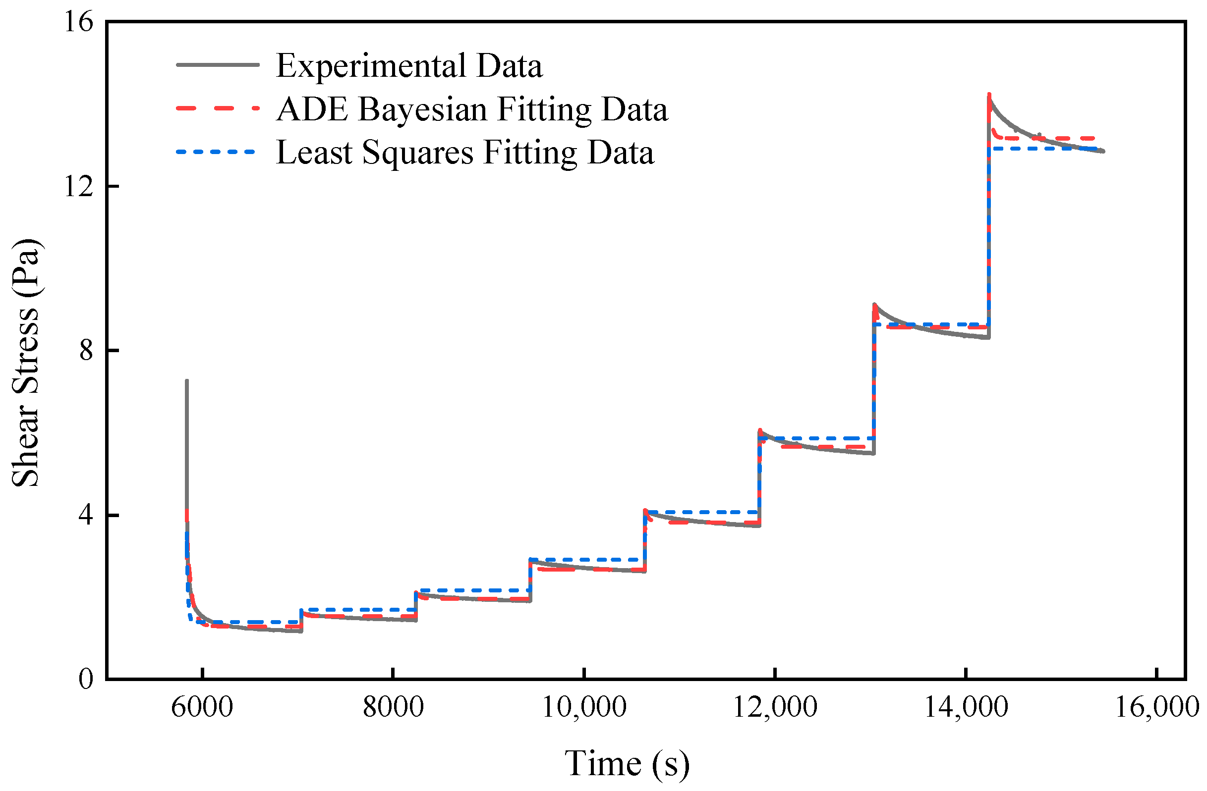
Figure 1 and Figure 2 show the fitting images of the Houska model based on the proposed thixotropic model parameter inversion method and the least squares method, using the stepwise increases in shear rate tests data of Daqing crude oil at 35 °C and Xianhe crude oil at 34 °C, respectively. As seen in Figure 1, the proposed thixotropic model parameter inversion method demonstrates a better fitting effect on the Houska model. The curve fitted by the least squares method significantly deviates from the experimental curve. This is because the initial values selected for fitting are far from the optimal ones, and, compared to the novel method, the least squares method is more sensitive to initial value selection and more prone to local optima. For the curves in Figure 2, the least squares method shows a smaller deviation from the measured curve but still does not fit the measured values as effectively as the novel method. Analysis indicates that, for Xianhe crude oil, the initial values selected for fitting are closer to the optimal values, resulting in good fitting curves for both methods. Observing Figure 1 and Figure 2, it can be seen that, after each step change in shear rate, the shear stress predicted by the Houska model quickly reached equilibrium, and the higher the shear rate, the earlier the equilibrium was reached. For the Houska model, its characteristic time of the structural parameter is $t=1/\left(a+b{\dot{\gamma }}^m\right)$, which is inversely proportional to the shear rate $\dot{\gamma }$. Consequently, an increase in shear rate reduces the characteristic time, leading to a shorter duration for the model’s shear stress to reach equilibrium.

4.1.2. Hysteresis Loop Tests

The fitting errors (MRE and RMSE) of the proposed thixotropic model parameter inversion method and the least squares method, based on the Houska model for the hysteresis loop tests of Daqing and Xianhe waxy crude oils, are, respectively, listed in

Table 3. MRE and RMSE of Houska model under hysteresis loop tests for Daqing Crude Oil.

T (°C)	RMSE		MRE
	LSM	Novel Method	LSM	Novel Method
32	2.14	2.01	10.30%	9.13%
33	1.16	1.13	8.62%	7.87%
34	0.60	0.56	8.85%	8.57%
35	0.24	0.19	9.32%	8.01%

and

Table 4. MRE and RMSE of Houska model under Hysteresis loop tests for Xianhe crude oil.

T (°C)	RMSE		MRE
	LSM	Novel Method	LSM	Novel Method
34	0.71	0.68	6.06%	5.76%
35	0.25	0.21	5.91%	5.09%
36	0.06	0.05	5.50%	2.40%
37	0.02	0.01	14.63%	10.08%

. All fittings in Table 3 were performed under the same set of given initial values, and all fittings in Table 4 were performed under another set of initial values. According to Table 3 and Table 4, for the hysteresis loop tests, under the same initial values, compared with the least squares method, the proposed thixotropic model parameter inversion method reduces the fitting error. The RMSE of Daqing crude oil and Xianhe crude oil decreased by an average of about 9.04% and 21.72%, respectively, and the MRE decreased by an average of 9.32% and 26.57%. This indicates that, for hysteresis loop tests, the proposed thixotropic model parameter inversion method also has higher accuracy and stability than the least squares method.

The fitting images of the Houska model, based on the proposed thixotropic model parameter inversion method and the least squares method, are shown in Figure 3 and Figure 4 for the hysteresis loop tests data of Daqing crude oil at 35 °C and Xianhe crude oil at 34 °C, respectively. Analysis of the images shows that both methods exhibit larger deviations during the stages of rapid stress drop and subsequent rise after the yield point. This is due to the inherent limitations of the Houska model itself.

In summary, the proposed thixotropic model parameter inversion method shows higher fitting accuracy and adaptability than the least squares method for different oil samples and experiments. This is because the least squares method is sensitive to initial parameters and is prone to local optima, especially in complex nonlinear models, where it may fail to find the global optimum, leading to larger fitting errors. In contrast, the proposed thixotropic model parameter inversion method efficiently searches for optimal initial values in a broad parameter space through ADE, effectively reducing the sensitivity to initial value selection. It also dynamically adjusts parameters and gradually optimizes the fitting results through Bayesian probabilistic sampling and error evaluation, thereby improving the model’s accuracy and stability.

4.2. Robust Analysis

To verify the robustness of the proposed thixotropic model parameter inversion method, the unknown parameters of Houska model were fitted under various initial values of model parameter, utilizing the shear rate step test data of Daqing waxy crude oil at 35 °C. The four sets of initial values employed in the fitting process are presented in

Table 5. Different initial values used for fitting the stepwise increases in shear rate tests of Daqing crude oil at 35 °C.

Initial Value	τy0	τy1	K	∆K	n	a	b	m
Initial Value 1	5.0000	20.0000	1.0000	7.0000	0.8000	0.1000	0.1000	0.5000
Initial Value 2	1.7715	20.0000	1.5681	5.7495	0.5373	0.0120	0.060	0.6739
Initial Value 3	1.2180	5.7823	1.0429	2.9948	0.5977	0.0062	0.0517	0.5643
Initial Value 4	0.6644	3.5645	0.5177	0.2400	0.6580	0.0004	0.0434	0.4547

, and the RMSE and MRE derived from fittings with different initial values are detailed in

Table 6. RMSE and MRE derived from fittings using various initial values for stepwise increases in shear rate tests of Daqing crude oil at 35 °C.

Initial Value	RMSE		MRE
	LSM	Novel Method	LSM	Novel Method
Initial Value 1	7.30	0.14	406.30%	4.79%
Initial Value 1	3.05	0.14	158.64%	4.79%
Initial Value 1	1.43	0.14	68.62%	4.79%
Initial Value 1	0.15	0.14	5.14%	4.79%

. As observed in Table 5 and Table 6, the errors of the least squares method exhibit significant variation with changes in initial values, with the RMSE fluctuating between 7.30 and 0.15 and the MRE ranging from 406.30% to 5.14%. In contrast, the errors of the proposed thixotropic model parameter inversion method remain essentially constant and are relatively small. This occurs because the least squares method is highly sensitive to changes in initial values. On the contrary, the proposed thixotropic model parameter inversion method utilizes the ADE algorithm for global search to optimize the initial values. And it updates the posterior distribution through Bayesian inversion, converging the parameters to a stable optimal region. This approach ensures a consistently reliable fitting effect. In addition, as the initial value 1 gradually changes to initial value 4, the error of the least squares method gradually decreases, which indicates that the given initial values gradually approach the optimal initial values. In Section 4.1 of this paper, the initial value used for fitting Daqing crude oil was initial value 2 in Table 5. For some temperatures, this initial value deviates significantly from the optimal initial value, resulting in large fitting errors.

4.3. Stability Analysis

To analyze the impact of Bayesian inversion iterations on the final values of model parameters, the changes in Houska model parameters with Bayesian inversion iterations were plotted in Figure 5 based on the stepwise increases in shear rate tests of Daqing crude oil at 35 °C. As shown in Figure 5, the parameters a, b, n, K, and m converge quickly and almost stabilize without significant oscillations, while other parameters converge relatively slowly. This indicates that the Bayesian optimization method has good stability in parameter adjustment. Even if some parameters change significantly in the initial stage, they eventually converge to stable values, showing good overall convergence and no trapping in local optima. The Bayesian method achieves a good balance between global search and local convergence, effectively adjusting parameters to obtain better fitting results.

Table 7. Fitted parameter values of Houska Model using the novel method based on the stepwise increases in shear rate tests data of Daqing crude oil from 32 °C to 35 °C.

T (°C)	τy0	τy1	K	∆K	n	a	b	m
32	0.3368	27.7009	2.0708	0.0120	0.4857	0.0125	0.0670	0.6488
33	0.7146	13.1443	1.0986	0.9600	0.5850	0.0094	0.0593	0.6786
34	0.0332	7.6314	0.8312	0.1244	0.6018	0.0135	0.0702	0.6369
35	0.0330	2.8256	0.2077	0.9600	0.7733	0.0276	0.1068	0.2052

shows the fitted model parameters of the Houska model by the proposed thixotropic model parameter inversion method, utilizing the stepwise increases in shear rate tests data of Daqing waxy crude oil from 32 °C to 35 °C. As can be seen from Table 7, the Houska model parameters fitted by Bayesian optimization show certain regularity. The primary yield stress parameter τ_y1 demonstrates a significant decrease with rising temperature, aligning with experimental findings and indicating that Bayesian optimization can precisely capture the temperature’s weakening effect on yield stress. Moreover, K, which reflects the shear thickening effect, also markedly decreases as temperature increases. The rheological behavior index n gradually rises with temperature, consistent with crude oil’s tendency to become less viscous at higher temperatures. The structure reformation rate constant, a, maintains a very small value, and shows no clear trend with temperature changes. This likely stems from the minimal structure reformation rate of waxy crude oil under flow conditions and the partially irreversible thixotropy of waxy crude oil. In summary, the Bayesian optimization method’s fitting parameters vary coherently with the oil’s rheological characteristics across different temperatures, enabling accurate modeling of the complex, temperature-dependent rheological behavior.

5. Conclusions

To address the issues of difficult initial value determination for model parameter fitting, susceptibility to local optimal solutions, and unstable fitting results, this study proposes a new method for Bayesian inversion of thixotropic model parameters integrated with ADE. Using the thixotropic test data of Daqing and Xianhe waxy crude oils, a comparative analysis was conducted between the proposed thixotropic model parameter inversion method and the traditional least squares method based on the Houska model. The results show that, for different oil samples and experimental conditions, the fitting errors of the new method are significantly smaller than those of the least squares method. Moreover, the proposed thixotropic model parameter inversion method can invert to obtain better thixotropic model parameters even when the initial parameter values are not ideal, or the parameter ranges are very broad while maintaining stable optimization capabilities. This resolves the issue of unknown parameter fitting in thixotropic models dependent on initial values. Additionally, the proposed thixotropic model parameter inversion method demonstrates good stability, with no violent oscillations in model parameters during the iterative inversion process, and good overall convergence. The model parameters obtained from inversion exhibit regularity with temperature changes, resolving the issues of local optimal solutions and unstable fitting results.

The proposed thixotropic model parameter inversion method surpasses the traditional least squares method in algorithm convergence, stability, and model fitting accuracy, addressing the challenge of fitting thixotropic parameters in waxy crude oils. And it can be extended to determining unknown parameters in other complex fluid rheological models.

References

1. Moud, A.A. Asphaltene induced changes in rheological properties: A review. Fuel 2022, 316, 123372. [Google Scholar] [CrossRef]
2. Li, M.; Chen, X.; Wang, Q.; Diao, D.; Zhang, Y.; Wang, C.; Zhang, L. Studying the effects of asphaltene oxidation on wax crystallization and rheological properties in waxy crude oils. Fuel 2024, 362, 130767. [Google Scholar] [CrossRef]
3. Ruwoldt, J.; Kurniawan, M.; Sørland, G.H.; Simon, S.; Sjöblom, J. Influence of wax inhibitor molecular weight: Fractionation and effect on crystallization of polydisperse waxes. J. Dispers. Sci. Technol. 2020, 41, 1201–1216. [Google Scholar] [CrossRef]
4. Zhao, S.; Cheng, Q.; Wang, S.; Liu, Y.; Qi, Y.; Wang, X. Molecular dynamics simulation of the microcosmic mechanism of resin effect on the gelling process of waxy crude oil. Fuel 2025, 384, 133927. [Google Scholar] [CrossRef]
5. Guo, L.; Han, X.; Lei, Y.; Wang, L.; Yu, P. Research on nonlinear rheological properties of waxy crude oil based on large amplitude oscillatory shearing. J. Pet. Sci. Eng. 2022, 213, 110444. [Google Scholar] [CrossRef]
6. Yin, X.; Liu, H.; Yang, C. Research Status and Prospect of Rheology of Waxy Crude Oil. Chem. Technol. Fuels Oils 2024, 60, 954–969. [Google Scholar] [CrossRef]
7. Houska, M. Engineering Aspects of the Rheology of Thixotropic Liquids. Ph.D. Thesis, Czech Technical University of Prague, Prague, Czech Republic, 1981. [Google Scholar]
8. Guo, L.; Zhang, J.; Sun, G.; Bao, Y. Thixotropy and its estimation of water-in-waxy crude emulsion gels. J. Pet. Sci. Eng. 2015, 131, 86–95. [Google Scholar] [CrossRef]
9. Dullaert, K.; Mewis, J. Thixotropy: Build-up and breakdown curves during flow. J. Rheol. 2005, 49, 1213–1230. [Google Scholar] [CrossRef]
10. Zhu, C.; Smay, J.E. Thixotropic rheology of concentrated alumina colloidal gels for solid freeform fabrication. J. Rheol. 2011, 55, 655–672. [Google Scholar] [CrossRef]
11. Van Der Geest, C.; Guersoni, V.C.B.; Merino-Garcia, D.; Bannwart, A.C. A modified elasto-viscoplastic thixotropic model for two commercial gelled waxy crude oils. Rheol. Acta 2015, 54, 545–561. [Google Scholar] [CrossRef]
12. Yahaya, J.; Kumam, P. New hybrid conjugate gradient algorithm for vector optimization problems. Comput. Appl. Math. 2025, 44, 163. [Google Scholar] [CrossRef]
13. Yuan, Q.; Liu, H.; Li, J.; Yu, B.; Wu, C. Study on the parametric regression of a multiparameter thixotropic model for waxy crude oil. Energy Fuels 2018, 32, 5020–5032. [Google Scholar] [CrossRef]
14. Yuan, Q.; Li, J.; Liu, H.; Yu, B.; Sun, D.; Deng, Y. Parametric regression of a multiparameter thixotropic model for waxy crude oil based on multiobjective strategy. J. Pet. Sci. Eng. 2019, 173, 287–297. [Google Scholar] [CrossRef]
15. Zhou, H.; Chen, C.; Feng, F.; Zhou, C.; Zhang, W.; Wu, W.-T. Study of Thixotropic Characteristics of a Kerosene Gel Propellant by Bayesian Optimization. Gels 2022, 9, 15. [Google Scholar] [CrossRef]
16. Ran, R.; Pradeep, S.; Acharige, S.K.; Blackwell, B.C.; Kammer, C.; Jerolmack, D.J.; Arratia, P.E. Understanding the rheology of kaolinite clay suspensions using Bayesian inference. J. Rheol. 2023, 67, 241–252. [Google Scholar] [CrossRef]
17. Ran, W.; Yue, B.; Liang, Y.; Guangming, D. Bayesian Compressive Sensing Identification of Mono-Frequency Sound Modes for In-Pipe Fan Noise. Acta Acust. 2025, 50, 187–200. (In Chinese) [Google Scholar] [CrossRef]
18. Ferragina, A.; de los Campos, G.; Vazquez, A.I.; Cecchinato, A.; Bittante, G. Bayesian regression models outperform partial least squares methods for predicting milk components and technological properties using infrared spectral data. J. Dairy Sci. 2015, 98, 8133–8151. [Google Scholar] [CrossRef]
19. Ennouri, K.; Ben Ayed, R.; Mazzarello, M.; Ottaviani, E.; Hertelli, F.; Azzouz, H. Classical and Bayesian predictions applied to Bacillus toxin production. 3 Biotech 2016, 6, 206. [Google Scholar] [CrossRef]
20. Brest, J.; Greiner, S.; Boskovic, B.; Mernik, M.; Zumer, V. Self-adapting control parameters in differential evolution: A comparative study on numerical benchmark problems. IEEE Trans. Evol. Comput. 2006, 10, 646–657. [Google Scholar] [CrossRef]
21. Brest, J.; Sepesy Maučec, M. Population size reduction for the differential evolution algorithm. Appl. Intell. 2008, 29, 228–247. [Google Scholar] [CrossRef]
22. Teng, H.; Zhang, J. Modeling the viscoelasto-plastic behavior of waxy crude. Pet. Sci. 2013, 10, 395–401. [Google Scholar] [CrossRef]
Figure 1. Inversion results of the Houska model for stepwise increases in shear rate tests of Daqing crude oil at 35 °C.
Processes 13 01320 g001
Figure 2. Inversion results of the Houska model for stepwise increases in shear rate tests of Xianhe crude oil at 34 °C.
Processes 13 01320 g002
Figure 3. Inversion results of the Houska model for hysteresis loop tests of Daqing crude oil at 35 °C.
Processes 13 01320 g003
Figure 4. Inversion results of the Houska model for Hysteresis loop tests of Xianhe crude oil at 34 °C.
Processes 13 01320 g004
Figure 5. The parameter iteration result of the Houska model for stepwise increases in shear rate tests of Daqing crude oil at 35 °C.
Processes 13 01320 g005