Article

A Collaborative Optimization Approach for Configuring Energy Storage Systems and Scheduling Multi-Type Electric Vehicles Using an Improved Multi-Objective Particle Swarm Optimization Algorithm

School of Information Engineering, Nanchang University, Nanchang 330031, China
*
Author to whom correspondence should be addressed.
Processes 2025, 13(5), 1343; https://doi.org/10.3390/pr13051343
Submission received: 9 April 2025 / Revised: 24 April 2025 / Accepted: 25 April 2025 / Published: 27 April 2025
(This article belongs to the Section Energy Systems)

Abstract

:
Energy storage systems (ESS) and electric vehicles (EVs) play a crucial role in facilitating the grid integration of variable wind and solar power. Despite their potential, achieving coordinated operational optimization between ESS and heterogeneous EV fleets to maintain grid stability under high renewable penetration poses a complex technical challenge. To address this, this study develops an integrated optimization framework combining ESS capacity planning with multi-type EV scheduling strategies. For ESS deployment, a tri-objective model balances cost, wind–solar integration, and electricity deficit. A Monte Carlo simulation algorithm is used to simulate different probabilistic models of charging loads for multiple types of EVs, and a bi-objective optimization approach is used for their orderly scheduling. An improved multi-objective particle swarm optimization (IMOPSO) algorithm is proposed to resolve the coupled optimization problem. Case studies reveal that the framework achieves annual cost reductions, enhances the wind–solar integration rate, and minimizes the power deficit in the system.

1. Introduction

China has prioritized its dual carbon strategy, aiming to achieve carbon peaking by 2030 and carbon neutrality by 2060 [1]. The power sector, responsible for 39.8% of national emissions through 4.46 billion tons of annual CO₂ output [2], urgently requires renewable energy expansion. Projections indicate that wind–solar installations will constitute over 60% of non-fossil capacity by 2030, exceeding 1200 GW [3]. However, the intermittent and fluctuating nature of these clean energy sources creates generation–demand mismatches that challenge grid stability [4]. To address this issue, large-scale ESS have emerged as critical infrastructure for balancing supply–demand discrepancies by storing surplus renewable generation and discharging during production deficits [5]. Concurrently, EVs have reached 20.41 million units nationally by 2023 [6], with an annual charging demand of 20.5 billion kWh, accounting for 6% of the total national electricity generation [7,8]. As a flexible scheduling resource, EVs [9], integrated with energy storage (ES) charging and discharging over multiple time scales, are expected to improve renewable energy absorption rates while lowering the investment costs of ESS [10]. The “hard–soft” integration of ESS and EVs provides an efficient solution for a future power system with high penetration of renewable energy. In this context, the question of how to configure ESS and schedule EV to maximize the efficiency of their coordinated operation while minimizing investment costs has become a critical challenge.

1.1. Literature Review

Recent advances have been made to improve the stability of wind–solar systems by optimizing the structure of the ESS. The integration of large-scale battery energy storage systems (BESS) into the grid [11] has been demonstrated to enhance the operational stability of high-penetration renewable energy systems. Digital twin hybrid storage solutions [12] have effectively managed microgrid power fluctuations within the 20–60 kW range, reducing the probability of supply shortages below 33%.
However, relying solely on ESS to absorb wind and solar power may lead to excessive capacity demand, which prompts a shift toward the collaborative optimization of multiple energy systems such as EVs. Ref. [13] demonstrated that integrated wind–BESS–EV systems can achieve a 28.6% increase in economic benefits. However, the study only considers a single form of renewable energy generation. Ref. [14] established a wind–solar–BESS multi-source system that achieves cost optimization by utilizing 76% of the EV load demand. Ref. [15] optimized BESS–EV in two stages to improve the peak-to-valley ratio by 46.73%. This highlights the technical advantages of integrating ESS with EV load scheduling, effectively reducing operational costs [16] and enhancing wind and solar energy integration [17]. Current research mainly focuses on single-objective optimization, which can only improve a single specific performance indicator and ignore other indicators [18].
However, practical engineering applications require the implementation of multi-objective optimization under multi-constraint scenarios, which cannot be solved by single-objective optimization frameworks [19]. Ref. [20] integrated cyber–physical–social systems to achieve the dual objectives of increasing renewable energy integration rates and reducing the costs of EV aggregators. Ref. [21] established a dual-objective model focusing on cost and carbon emissions, effectively reducing the design capacity of BESS. However, it should be noted that many multi-objective optimization problems utilize fixed weights, which can result in a decline in the precision of the Pareto front solutions.
In addition to the objective design challenges, algorithms for solving such problems have different technical paths and common bottlenecks. In [22], the particle swarm optimization (PSO) algorithm was used to solve the key parameters and optimize the energy allocation between the wind–solar–ES and the EV. In [23], a simulated annealing algorithm was used to reduce the grid loss of EV charging to the grid. In [24], voltage deviation and active power loss were improved by 11.04% and 1.37%, respectively, using genetic algorithms. Rule-based metaheuristic algorithms are mainly used to solve single-objective or multi-objective problems.
In summary, there are two main problems in the existing studies. Firstly, conventional methods consider EV clusters as homogeneous demand-side entities, which fail to effectively account for the heterogeneous characteristics of market participants, including but not limited to differences in daily driving mileage, charging duration distribution, and other key parameter variations. Secondly, most studies employ rule-based metaheuristics algorithms to solve single or multi-objective problems. These approaches are inherently limited by the curse of dimensionality and by computational complexity constraints. These approaches often encounter premature convergence and local optima when addressing nonlinear wind-solar storage-load multi-constraint, multi-objective problems [25].

1.2. Contributions

To address existing research limitations, this study investigates a collaborative optimization framework for the configuration of ESS and the scheduling of multi-type EVs. The main novelties and contributions are summarized as follows:
(1)
A multidimensional collaborative optimization framework is proposed for high-penetration renewable energy systems, which uncovers the nonlinear coupling mechanisms between the configuration of ESS and the scheduling of multi-type EVs. This framework aims to maximize the coordinated operation of ESS and EVs, thereby enhancing the integration of renewable energy.
(2)
A differentiated charging demand model for private cars, taxis, and buses is developed based on real-world operational data, with the Monte Carlo algorithm employed for load forecasting. This approach improves upon existing EV studies by better capturing user behavior heterogeneity and enhancing the accuracy of time distribution modeling for charging demand.
(3)
An IMOPSO algorithm is proposed, combining dynamic crowding distance Pareto front updates, adaptive inertia weights, and entropy-weighted technique for order preference by similarity to an ideal solution (TOPSIS) selection. This effectively addresses high-dimensional nonlinear constraints and fixed weight limitations, outperforming non-dominated sorting genetic algorithm-II (NSGA-II) and traditional multi-objective particle swarm optimization (MOPSO) in convergence speed and solution uniformity.
This article is organized as follows. Section 2 presents the mathematical modeling of the wind–solar storage-load system. Section 3 builds on the proposed multi-objective collaborative optimization framework, including the design of the IMOPSO algorithm. Section 4 discusses the experimental results and comparative analysis. Finally, Section 5 concludes the research findings.

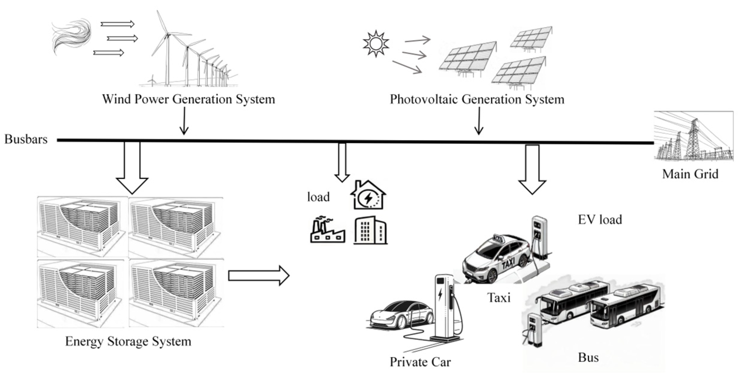
2. Wind–Solar Storage-Load System Model

The system is primarily composed of wind and solar power sources, an ESS, EV load and other load, as shown in Figure 1.

2.1. Wind Power Generation Model

The efficiency of wind power generation is influenced by several factors, with wind speed being of particular significance. Studies in this area have demonstrated that the output power of a wind energy system exhibits a segmented functional relationship with wind speed, as shown by
P W T = 0 v < v c i | | v > v c o v v c i v R a v c i p W T R v c i v < v R a P W T R v R a v < v c o
where P W T is the output power of the wind turbine (WT); v ,   v c o ,   v c i   , and v R a denote the wind speed, cut-out wind speed, cut-in wind speed, and rated wind speed; and P W T R represents the rated output power of the WT.

2.2. Photovoltaic Power Generation Model

The efficiency of photovoltaic (PV) power generation is contingent on several factors, but the solar irradiance and the operating temperature of the photovoltaic cell are the primary factors affecting the output power of the system. The relationship between these variables is expressed by the following (2):
P P V = P P V   R   G g [ 1 + k ( T t T m a ) ] / G m a
where P P V   represents the PV output power, with P P V R as the rated output power; G g represents the current irradiance; G m a is the irradiance under standard test conditions; k is the temperature coefficient of power; T t is the current operating temperature; and T m a is the temperature under standard test conditions.

2.3. ESS Model

The ESS is vital to the overall system, as it not only balances the load effectively but also ensures the stable operation of wind and solar power generation, thereby enhancing the integration of renewable energy.
The state of charge (SOC) of the ESS at time t , denoted as s o c ( t ) , is defined as
s o c   ( t ) = E t   E Z     ×   100 %
where E t represents the stored energy in the ESS at time t   and   E z   represents the rated capacity of the ESS.
The dynamic calculation expression for the SOC during charging and discharging is given by
  s o c   ( t ) = s o c ( t 1 ) η c 0 α Δ T P C ( t ) d t E z P C ( t ) 0                                   s o c ( t 1 ) 0 α Δ T P C ( t ) d t E z η f   P C ( t ) > 0
where   η c   and η f represent charging efficiency and discharging efficiency, respectively,   P c ( t ) denotes the charging and discharging powers, and α is the total number of sampling intervals.

2.4. Multi-Type EVs Flexible Load Model

2.4.1. Modeling of Daily Driving Distance

Daily driving distance is a crucial parameter for assessing the daily energy consumption of EVs and plays a significant role in determining the charging duration. Studies indicate that the distribution of daily driving distances for multi-type EVs exhibits distinct probabilistic characteristics. These characteristics can be mathematically represented by the following expression:
f ( x ) = 1 2 Π σ a e ( x μ a ) 2 2 σ a 2 λ e λ x 1 x m i n x m a x
where x is the daily driving distance, μ a   and σ a   denote the mean and standard deviation, respectively, x m a x   and   x m i n   denote the maximum and minimum driving distances of the EV, respectively, and λ is the distribution parameter.

2.4.2. Model of Charging Start Time

The charging start time of multi-type EVs depends on various factors, including user work schedules, vehicle characteristics, and usage patterns. Its distribution exhibits distinct temporal variations, with probabilistic behavior differing across time intervals. The probability distribution is defined as follows:
f ( t ) = 1 2 Π σ b e ( t μ b ) 2 2 σ b 2 1 t l a s t t e a r l y
where t represents the starting charging time of multi-type EVs,   μ b and σ b denote the mean and standard deviation of the charging start time for an exponential distribution, and t e a r l y and t l a s t denote the earliest and latest charging times for a uniform distribution of charging start times.

2.4.3. Charging Power for EVs

Charging power is intrinsically linked to the charging mode, which can generally be categorized into constant current charging, multi-stage charging, and pulse charging. For this study, it is assumed that the charging power for multi-type EVs is a constant value, denoted as P d .

2.4.4. Charging Duration

The initial SOC of an EV is calculated based on the ratio of the distance traveled to the nominal distance extracted probabilistically for each electric vehicle. In this paper, it is assumed that the initial SOC of an EV is equal to the remaining SOC at the end of the previous trip, and the calculation process of the initial SOC is summarized as follows:
  S O C 1 = 1 x x m a x × 100 %
where S O C 1 represents the initial SOC of the EV at the start of charging.
The charging duration is given by
T = ( S O C 2 S O C 1 ) E P d η e v
where T represents the charging duration, S O C 2 denotes the SOC at the end of charging, η e v denotes the charging efficiency of the EV, and E is the rated capacity of the EV’s battery.

2.5. Multi-Type EVs Load Setting

2.5.1. Electric Private Car

According to the annual transportation report by the Beijing Transportation Research Institute [26] and supplementary regional survey data, fast charging is primarily used during daytime hours. Private car charging initiation follows a uniform distribution during working hours, while post-working hours see a shift to normal distribution, with a marked increase in slow charging frequency. On weekdays, the average daily driving distance for electric private cars is 50.55 km, increasing to 55.56 km on non-working days. The nominal mileage is now commonly around 510 km. The driving distance is modeled using an exponential distribution, reflecting variations in travel demand and patterns between workdays and non-workdays.

2.5.2. Electric Taxi

As shown in Table 1, a thorough investigation into the operational efficiency of electric taxis within a specific region has revealed that a single charge is not sufficient to meet daily operational needs. Consequently, taxi drivers typically adopt a strategy of charging twice daily. The charging time is generally split evenly between the lunch break (11:00–14:00) and after the evening shift (02:00–04:00). The mean daily distance traveled by this taxi was normally distributed, with a mean value of approximately 275 km, reflecting the typical high-frequency use of electric taxis in this operating environment. This distance underscores the high utilization of electric taxis and provides a theoretical foundation for their deployment.

2.5.3. Electric Bus

A review of the current technical specifications of the deployed electric buses indicates that, under normal operating conditions, they generally do not require midway recharging. Consequently, these buses generally necessitate a single daily charge to satisfy their energy requirements. The necessity for charging is not fixed, due to the flexibility to charge after completing a scheduled route or during off-hours. Furthermore, surveys conducted on electric bus operations in specific regions have shown that the distance traveled is consistently between 150 and 200 km per day. Buses are now generally rated at around 180 km. This consistent distance travel is indicative of the operational efficiency and predictable usage patterns exhibited by electric buses, which are critical factors in facilitating their integration into EV scheduling.

2.6. Monte Carlo-Based Multi-Type EV Charging Load Forecasting Process

The Monte Carlo method is a numerical technique based on random sampling, leveraging many samples to simulate complex processes and improve result accuracy through extensive computational simulations [27]. In this paper, a model considering various factors affecting EV charging loads is developed to determine the charging energy and duration for multi-type EVs. Then, the total charging load is calculated by aggregating the charging demand of all vehicles during their respective charging periods, as shown in (9):
      P E V = k = 1 3 t = 1 24 i = 1 N 1 P i j k
where P E V represents the total charging load of EVs at time t , N 1   denotes the number of EVs, and P i j k refers to the charging power of the i EV of type k at time t . The solution process of the Monte Carlo algorithm in this paper is shown in Figure 2:

3. Collaborative Optimization for the Configuration of ESS and the Scheduling of EVs

This paper adopts a collaborative optimization framework aimed at achieving the collaborative optimization of ESS and EVs. In the first stage, by integrating the predicted loads of multi-type EVs with the measured data from other loads, the overall system load curve is constructed, which in turn enabled the collaborative optimization of the energy storage system’s capacity configuration and operational strategy. In the second stage, based on the determined ESS configuration, the loads of multi-type EVs are converted into decision variables, allowing them to respond to time-of-use pricing mechanisms while actively adapting to the operational characteristics of the ESS. This formed a collaborative optimization of ESS configuration and EVs scheduling. Through this approach, the overall performance of the new power system is enhanced.

3.1. Optimization Configuration of ESS

The multi-objective evaluation framework established for optimizing the configuration of ESS is defined as follows:
O p t i m a l   f 1 = min   C T , max   R , min H
where C T represents the annual total cost of the wind–solar-storage system (unit: CNY), R denotes the wind–solar integration rate (unit: %), and H refers to the system electricity deficit (unit: kWh).

3.1.1. Annual Total Cost

The annual total cost includes all expenditures over the system’s life cycle, such as initial capital investment in wind–solar storage, along with ongoing operational and maintenance costs.
C T = C c o n s + C m i t n C B E
Here,   C c o n s represents the construction cost, C m i t n denotes the annual maintenance cost, and C B E refers to the additional annual revenue cost for ESS.
(1)
Construction Cost
The construction cost of the wind–solar storage system is calculated using the following formula:
          C cons = C c o n s P V + C c o n s W T + C c o n s C C c o n s P V = F P V P P V R i ( 1 + i ) N ( 1 + i ) N 1 C c o n s W T = F W T P W T R i ( 1 + i ) N ( 1 + i ) N 1 C cons C = ( F R R C + F P P C ) i ( 1 + i ) N ( 1 + i ) N 1
where C c o n s P V , C c o n s W T , and C c o n s C represent the annual total construction costs for the PV, WT, and ESS, respectively; F P V and F W T denote the construction costs per unit power for the wind–solar system, respectively; F R and F P refer to the construction costs per unit capacity and per unit power for the ESS, respectively; R C and P C represent the rated power and rated capacity of the ESS, respectively; N is the total number of years of operation; and i is the discount rate.
(2)
Maintenance Costs
The annual maintenance costs of wind–solar storage system are as follows:
C m i t n = C m i t n P V + C m i t n W T + C m i t n C C m i t n P V = l = 1 N M P V P P V N ( 1 + i ) l 1 C m i t n W T = l = 1 N M W T P W T N ( 1 + i ) l 1 C m i t n C = l = 1 N M R R C + M P P C N ( 1 + i ) l 1
where C m i t n P V , C m i t n W T , and C m i t n C represent the total annual maintenance costs for the PV, WT, and ESS, respectively; M P V and M W T represent the unit maintenance costs per unit power for the wind–solar system, respectively; and M R and M P represent the unit maintenance costs per unit capacity and per unit power for the ESS, respectively.
(3)
Incremental Annual Grid Revenue from the ESS
ESS makes a profit by transferring power through charging and discharging, which is calculated as follows:
C B E = t = 0 T 1 w t P C ( t ) Δ t
where   w t represents the time-of-use electricity price and T 1 denotes the total time duration during which the ESS feeds electricity into the grid.

3.1.2. Wind–Solar Integration Rate

To enhance the ESS’s role in renewable energy integration, optimizing the wind–solar integration rate is a key objective. This study presents a comprehensive optimization framework that incorporates daily generation profiles year-round to maximize the wind–solar integration rate. This approach effectively addresses the variability of wind–solar resources, enabling efficient utilization throughout the year.
R = 0 8760 [ P P V S ( t ) + P W T S ( t ) ] t 0 8760 [ P P V ( t ) + P W T ( t ) ] t × 100 %
Here,   P W T S and P P V S represent the actual consumption power of wind–solar energy at time t , respectively.

3.1.3. System Electricity Deficit

In new power systems, the intermittent nature of wind–solar generation often leads to situations where the power supply cannot fully meet demand, necessitating the use of conventional energy sources, such as thermal power, to balance supply and demand. The deployment of ESS can significantly mitigate the power deficit, enhancing the reliability and stability of the system during the transition to a power grid with high renewable energy penetration.
H = t Psp [ P G r ( t ) P P V ( t ) P W T ( t ) P C ( t ) ]   Δ t  
Here, H represents the system electricity deficit, P G r ( t ) denotes the system load power, and Psp denotes the system power shortage periods.

3.1.4. Constraints

(1)
Load Balance Constraint
The load balance constraint is one of the core constraints in the wind–solar storage system model. It ensures that the combined generation from wind–solar storage system meets the load demand at each time period. In this case, the total load consists of EV load and other loads:
P G r ( t ) = P E V ( t ) + P O T ( t ) P G r ( t ) + P G ( t ) = P P V ( t ) + P W T ( t ) + P C ( t )
where   P G ( t ) is the curtailment power of the wind–solar storage system at time t and P O T ( t ) is the other load at time t .
(2)
ESS Constraints
The ESS has both upper and lower limits on its output power, as well as cycle life characteristics. The following constraints must be adhered to:
0 | P C | P C _ M A X T B 15   | |   T M A X 5000
where P C _ M A X represents the maximum charging and discharging power of the ESS.
(3)
System Deficit Constraint
The electricity deficit of the system must not be negative at any time, thereby ensuring the rationality and feasibility of the system optimization:
H 0

3.2. Multi-Type EV Optimization Dispatch Objective Function

Upon the completion of the optimization of the ESS configuration, the results are utilized to further optimize the dispatch of EV charging, thereby enhancing the overall performance metrics of the system. The established multi-objective evaluation framework is as follows:
O p t i m a l   f 2 = min   C E V   ,   max     L r
where C E V represents the charging cost for EV users (unit: CNY) and Lr denotes the load factor (unit: %).

3.2.1. Charging Cost for EV Users

In the orderly deployment of multi-type EVs, it should be ensured that users receive the best economic benefit. The charging costs are calculated using the following formula:
C E V = t = 1 T 2 w t P E V ( t ) Δ t
where T 2 is the total duration for which the EV participates in the scheduling process.

3.2.2. Load Factor

The load factor serves as a key performance indicator for the load curve following the optimization dispatch of multi-type EVs. A higher load factor signifies a more uniform distribution of load across different time periods, resulting in a reduced peak-to-valley variation [15]. The mathematical expression is given as follows:
L r = d = 1 365 P aver 365 P G r ,   max × 100 %
where P a v e r represents the average load and P G r , m a x denotes the peak load.

3.2.3. Constraints

(1)
Load Balance Constraint
The power balance equation must be maintained at every time step in the system when multi-type EVs are scheduled in a coordinated manner.
  P G r ( t ) = P E V ( t ) + P O T ( t ) P G r ( t ) = P P V ( t ) + P W T ( t ) + P C ( t ) P G ( t )
(2)
Multi-Type EVs Load Constraints
Given the varying parameter characteristics of multi-type EVs, it is necessary to ensure the accuracy of the research results by imposing the following constraints on each vehicle type:
0 P E V P E V α , M A X S E V α , M I N S E V S E V α , M A X N E V α , M I N < N E V < N E V α , M A X
where P E V α , M A X represents the maximum charging load of EV type α , S E V α . M I N and S E V α . M A X denote the minimum and maximum SOC of EV type α , respectively, and N E V α . M I N and N E V α . M A X represent the minimum and maximum number of EV type α , respectively.

3.3. Solution Algorithm—IMOPSO

3.3.1. Classical PSO Algorithm

The classical PSO algorithm is a stochastic optimization method that explores the solution space. The initial population consists of particles randomly distributed within the search space [28]. Throughout the optimization process, particles update their velocity and position by combining individual historical information with knowledge shared by the swarm. In every iteration, the velocity and position of each particle are updated based on two key “optimal positions”—the individual best (pbest) and the global best (gbest)—using the following update rules:
v i j k + 1 = w k v i j k + c 1 r 1 ( p b e s t i j k x i j k ) + c 2 r 2 ( g b e s t i j k x i j k )
x i , j k + 1 = x i , j k + v i , k k + 1
where w represents the inertia weight,   c 1 and c 2 are the individual cognitive and social learning factors, respectively, k is the current iteration, r 1 and   r 2   are random values uniformly distributed within the interval [0, 1], v i j   k and x i j   k refer to the j-th component of the velocity and position vector of the i-th particle at iteration k , respectively, and p b e s t i j   k and   g b e s t i j   k are the j-th component of the best position achieved by the i-th particle and the global best position of the swarm at iteration k , respectively.
Due to the inherent nonlinearity, dynamics, and uncertainty of the ESS allocation and EV scheduling problems, the traditional algorithm tends to converge to the local optimum prematurely, thus limiting its ability to find the global optimum. The main challenges include (1) the lack of a theoretical basis for inertia weight selection and (2) the inefficiency of the fitness ranking mechanism in multi-objective optimization when dealing with non-dominated solution sets [29]. To address these issues, this paper improves the Pareto updating strategy, optimizes the inertia weighting mechanism, and selects the optimal solution using the entropy weighting method. These improvements enhance the global optimization capability and adaptability of the algorithm, which is conducive to exploring and utilizing the solution space more efficiently and ultimately achieving the global optimal solution.

3.3.2. Pareto Solution Set Update Strategy

In multi-objective optimization, crowding distance is essential for updating the Pareto front [30]. However, traditional methods are limited by exchange of information only between adjacent individuals, which can degrade solution distribution and uniformity. To overcome this, this paper proposes a particle sorting and selection mechanism using dynamic crowding distance, improving both global optimization and solution distribution. The dynamic crowding distance is computed by summing the distances between a particle and its two nearest neighbors. Pareto solutions are ranked by descending crowding distance, and solutions with the smallest distances are iteratively removed until the desired number of solutions is reached.
d x i , k = | f 1 x i f 1 x k | f 1 m a x + | f 2 x i f 2 x k | f 2 m a x + | f 3 x i f 3 x k | f 3 m a x
Here, d ( x i , k ) represents the distance between particle x i and x k ; k = 1,2 , , N; f 1 ( x i ) , f 2 x i , and f 3 ( x i ) are the three objective function values of particle x i ; and f 1 m a x , f 2 m a x , and f 3 m a x are the maximum values of the three objective functions across all particles.

3.3.3. Adaptive Adjustment of Inertia Weight

The inertia weight parameter is crucial for algorithm performance. A larger value promotes global exploration but may reduce solution precision, while a smaller value enhances local search but risks premature convergence to suboptimal solutions [31]. To address this, the proposed enhanced algorithm employs an adaptive inertia weight strategy, optimizing particle search behavior. Particles with higher fitness are directed toward local searches for greater accuracy, while those with lower fitness are assigned larger weights to facilitate broader exploration, improving global optimization. This mechanism maintains solution diversity and ensures balanced convergence, optimizing exploration and exploitation.
w = w m i n + ( w m a x w m i n ) ( s i s m i n ) s a s m i n     s i s a v                                                     w m a x                                             s i > s a v
Here, w m i n and w m a x represent the lower and upper bounds of the inertia weight coefficient, respectively, s i   denotes the fitness of the current particle, and s a v and s m i n refer to the average and minimum fitness values of the current particle swarm, respectively.

3.3.4. Selection of the Optimal Solution

In the final decision-making phase of the multi-objective optimization system, this paper employs the TOPSIS method based on entropy weighting to determine the optimal solution. The process consists of the following steps.
First, the data in the Pareto solution set is normalized to eliminate the impact of different units of measurement across the objective functions. This normalization process follows (29):
f i k = f k m a x f i k f k m a x f k m i n ,     i = 1,2 , 3 , , n
where n represents the number of solutions in the Pareto set, f i k and f i k denote the actual and normalized values of the k-th objective function for particle i , respectively, and f k m a x and f k m i n represent the absolute positive and negative ideal solutions for the k -th objective function.
Next, the entropy-based method is used to calculate the weights for each objective, as shown in (30):
λ k = 1 E k m i = 1 n E i E k = i = 1 n P i k ln P i k ln ( n )
where
P i k = f i k i = 1 n f i k
where E k represents the information entropy of the k -th attribute and λ k denotes the weight of the k -th attribute.
Finally, based on the determined weights for each objective, the improved MOPSO algorithm further calculates the distance and closeness of each solution to the ideal solution.
  S i + = k = 1 m ( λ k f i k λ k f k + ) 2       S i = k = 1 m ( λ k f i k λ k f k ) 2       C i = S i S i + + S i
Here, S i + and S i represent the positive and negative ideal distances for particle i , respectivel, and C i denotes the closeness of particle i .

3.3.5. Solution Process

The solution process of the IMOPSO algorithm in this paper is shown in Figure 3:

4. Simulation Analysis

4.1. Simulation Setting

The energy system depicted in Figure 1 is utilized for simulation analysis to validate the effectiveness of the proposed method in optimizing the configuration of ESS and the scheduling of multi-type EVs. In this system, historical wind and solar power generation data are shown in Figure 4, where each curve of different color represents the power output on different dates. Both wind and solar power generation exhibit significant volatility, with the annual volatility intensity of wind power being 2.3 orders of magnitude higher than that of solar power. The time-series analysis reveals the complementary characteristics of the wind–solar system; during the daytime, the solar system achieves efficient energy conversion, while wind power contributes 33% to the total power generation at night.
Furthermore, the parameters of the IMOPSO algorithm, designed using the MATLAB R2024a platform, are set as follows; the initial population size is 100 individuals, the maximum number of iterations is 200, and the archiving capacity for non-dominated solutions is 100 sets. Additional parameters are provided in Table 2.

4.2. Case Study Analysis

To validate the effectiveness of the proposed method, three operating scenarios were established for comparative analysis:
  • Scenario 1: only optimizing the configuration of ESS;
  • Scenario 2:optimizing the configuration of ESS and the scheduling of single-type EVs;
  • Scenario 3: optimizing the configuration of ESS and the scheduling of multi-type EVs.
Table 3 shows the simulation results of the three scenarios. Compared to Scenario 1, Scenario 3 reduces annual total cost by 17.42%, increases wind–solar integration rate by 4.91%, decreases power deficit by 54.76%, lowers user charging costs by 30.21%, and improves load factor by 5.66%. Compared to Scenario 2, Scenario 3 reduces annual total cost by 10.49%, increases wind–solar integration rate by 2.92%, decreases power deficit by 40.98%, lowers user charging costs by 19.79%, and improves load factor by 2.97%. These results demonstrate that the optimized ESS configuration, combined with the orderly scheduling of multi-type EVs, not only enhances the economic performance of the system but also significantly improves energy consumption efficiency and power supply–demand balance, thereby strengthening the overall system performance.

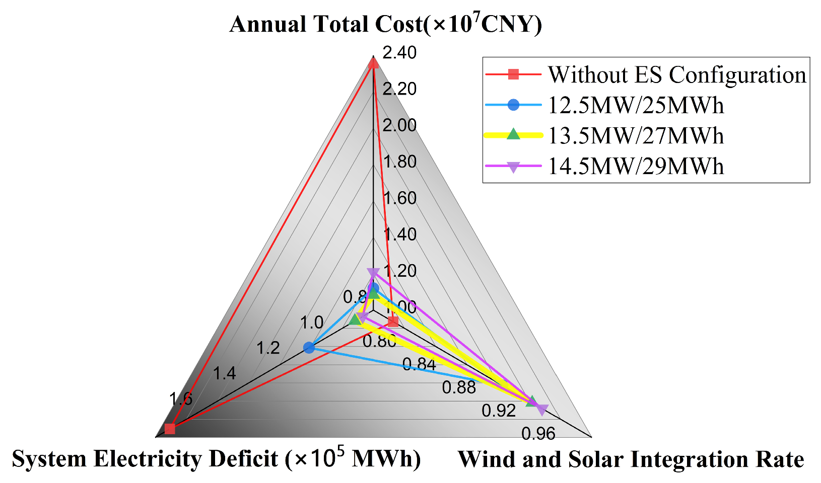
4.3. Optimization Results of ESS Configuration

Figure 5 illustrates the typical daily output of wind–solar energy and the operation of the ESS. The maximum output is observed to be 29.2 MW at 14:00, while the minimum is recorded as 19.5 MW at 03:00, with a peak-to-valley difference of 33.21%. The operational profile demonstrates “source–load inversion” during 00:00–06:00 and 09:00–16:00, while revealing a 12.3 MW power deficit during the evening peak period (17:00–21:00). This pattern underscores the mismatch between wind–solar generation output and load demand. Load analysis (red curve) shows two demand peaks—a daytime peak at 10:00 (26.3 MW) and an evening peak at 20:00 (26.9 MW)—with a subsequent decline to 19.3 MW during the nighttime period. This mismatch presents opportunities for optimizing ESS operation. The ESS achieved efficient energy transfer through time-of-use pricing implementation for charge/discharge operations, storing 24.81 MWh by 17:00 and delivering 14.42 MWh during peak demand periods (17:00–22:00). Quantitative analysis shows that the system enables an additional 17.67 MWh of wind–solar integration, generating CNY 30,185.1 in revenue and reducing CO2 emissions by 15.9 tons on the same day.
A comparative analysis is conducted to evaluate ESS configurations with capacity variations, drawing upon established findings. The optimal configuration is found to result in a 56.85% reduction in total annual costs, a 17.5% improvement in wind–solar integration rate, and a 51.89% reduction in power deficits compared to the scenario without ESS deployment. As shown in Figure 6, approaching the optimal ESS capacity creates a positive cost–benefit balance. Beyond that point, efficiency drops, and adding 1 MW of ESS reduces wind–solar integration growth from 0.98% to 0.21%, and cost change from −3.74 × 10⁵ CNY/MW to +1.03 × 10⁶ CNY/MW. The optimal solution is selected using the TOPSIS method, with the target weights assigned as follows: annual cost (0.497), wind–solar integration rate (0.272), and electricity deficit (0.231). The comprehensive performance index reached 0.873, representing a 62.4% improvement over the baseline. This provides a robust model for optimal ESS planning in high renewable energy grids.

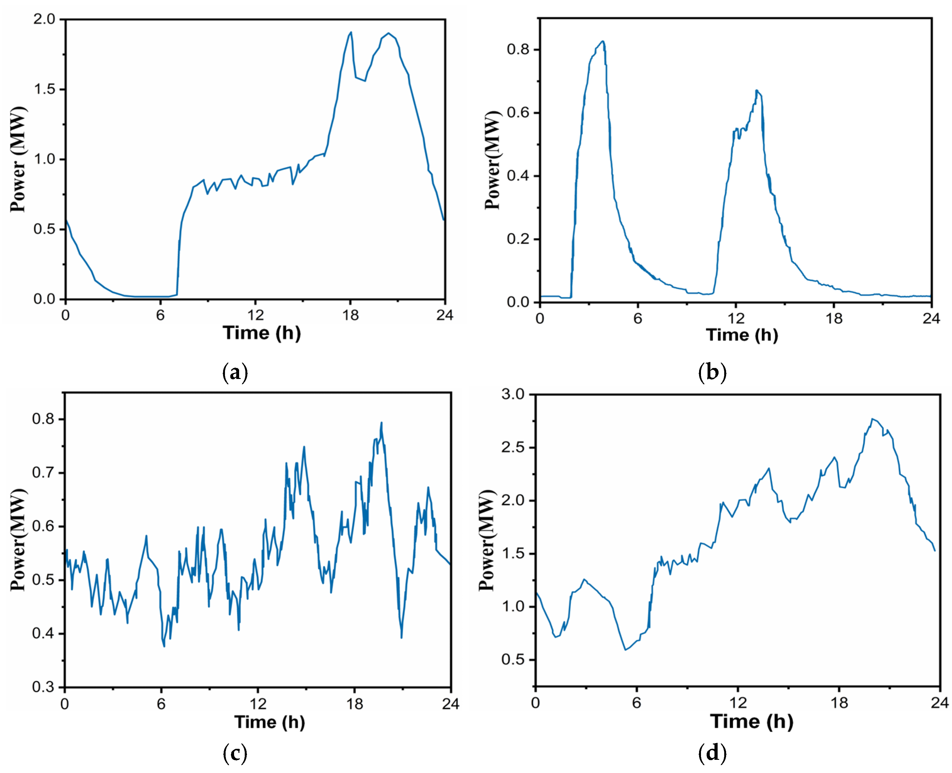
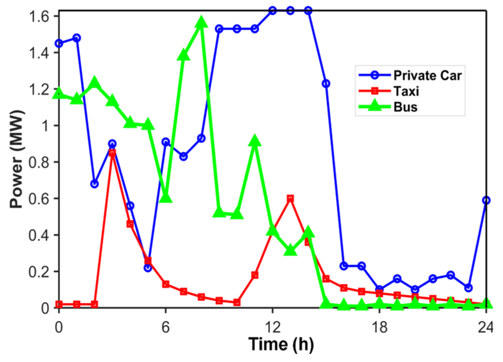
4.4. Monte Carlo Simulation for Multi-Type EV Load Forecasting

The private car charging load peaked at 1.89 MW at 20:00 and decreased to a minimum of 0.01 MW at 07:00. During time period 1 (16:00–21:00), the load increases significantly due to the concentration of after-work charging demand. During time period 2 (21:00–07:00), the load gradually decreases as those opting for fast charging complete their charging and those opting for slow charging have a slower SOC ramp-up, resulting in lower overall power demand. This trend reflects the reduction in charging demand during the night. A peak occurs during the third hour (07:00–16:00) as vehicles that have not been charged overnight start charging before the morning peak, after which the load stabilizes. Figure 7b shows the bimodal distribution of taxi charging demand, with double peaks at 04:00 (0.85 MW) and 14:00 (0.69 MW), which is influenced by fleet operations and time-of-use price. The bus charging load profile is highly variable, with no significant peak charging periods. Loads fluctuate between 0.37 MW and 0.79 MW. This variation is a direct result of the characteristics of bus operations and charging strategies. Adaptive charging strategies can be used by bus operators to meet the operational demands of different routes and schedules, to reduce the risk of load concentration, and to optimize the charging demand distribution.
Analysis of the total EV load profile shows that the total load is influenced by the combined charging demand of all vehicle types. The trend of total load is closely related to private car load. Fluctuations in total load are more pronounced than for private cars or taxis, mainly due to the charging behavior of buses. The total load shows multiple peaks, especially between 02:00 and 04:00 and 11:00–14:00, which is mainly due to the charging pattern of taxis. These fluctuations reflect the different charging needs of different types of EVs throughout the day. Two situations present themselves:
  • Situation 1: disordered EV charging;
  • Situation 2: ordered EV charging.
As shown in Figure 8, incorporating multi-type EVs into the system presents both challenges and opportunities for optimizing wind–solar energy consumption and improving system economics. In Situation 1, characterized by disordered EV charging, significant operational constraints are observed. The ESS reaches its maximum charging capacity at 04:00 h due to the uncontrolled EV demand during the night, resulting in insufficient wind–solar absorption reserves during the day. This configuration leads to a 34.5% increase in wind–solar curtailment compared to situation 2. Additionally, a 13.26 MWh peak-hour electricity deficit in the grid highlights the dual inefficiencies of this scheme; the inability to efficiently utilize the ESS undermines wind–solar integration, and the rigid charging model exacerbates peak–valley load differentials, ultimately reducing economic benefits.
Situation 2 addresses these challenges through the implementation of orderly EV scheduling. In this scenario, the system achieves two ESS charge/discharge cycles that are aligned with the wind–solar generation profile, based on the varying charging times of the multi-type EVs. This optimized scheduling increases wind–solar integration by 38.7% and improves the system load factor to 85.9%. It completely eliminates daily power shortfalls, enhances wind and solar energy uptake without curtailing power, and reduces charging costs for EV users by CNY 16,510 on the same day. Simultaneously, the ESS strategically discharges power between 18:00 and 24:00 to support evening peak demand, demonstrating effective energy arbitrage. The scenario analyses show that the orderly scheduling of multi-type EVs transforms their demand into a flexible resource, enabling the grid to maintain balance and achieve a combined optimization of wind–solar integration, energy efficiency, and economic returns.
The private car scheduling strategy shows a clear feature of charging concentration during the daytime, with a maximum charging power of 1.62 MW to relieve the evening peak pressure. In total, 50.3% of the charging load is shifted 2–3 h ahead to the period of high wind–solar generation, while 41.1% of the demand is shifted after 00:00, combined with delayed slow-charging initiation after evening returns. This strategy has been shown to achieve a peak shaving effect of 90.6%. During the 20:00 peak load period, the demand-side response mechanism adjusts the charging power to near-zero levels, effectively curbing 2.7 MW of potential peak load growth and ensuring grid stability.
Electric taxis, as essential transportation components, present a dual-peak charging characteristic (02:00–09:00 and 10:00–16:00) with maximum charging power of 0.87 MW, demonstrating coupling with system dispatch requirements. Data analysis reveals 92.3% off-peak charging concentration. Projected 2.8-fold fleet expansion combined with intelligent charging scheduling could additionally absorb 23.6% of curtailed wind–solar power during nighttime and increase annual energy utilization by 1.55 GWh.
Electric buses exhibit superior scheduling flexibility, dynamically adjusting charging plans based on operational requirements. As illustrated in Figure 9, 73.6% of their charging loads concentrate within 00:00–09:00, with only 16.4% daytime supplementary demand and emergency charging intensity reduced to 1.2 kW/vehicle during evening peaks. Orderly scheduling with other vehicle types achieves 99.8% wind–solar integration rate and reduces EV user charging costs to 29.5% on the same day.
This study predicts the demand response of multi-type EVs, performs load shifting, and matches the output of a wind–solar-storage system, which significantly improves the operational efficiency of a modern power system. The proposed model innovatively converts traffic loads into grid regulation resources, providing a 6% flexible regulation capability for grids with high renewable energy penetration.

4.5. Sensitivity Analysis of Key Parameters

In this study, a quantitative sensitivity analysis based on the univariate perturbation method was conducted to ascertain the marginal effects of EV penetration, time-of-use price, and ESS cost pass-through on the total annual cost of the new power system, the wind–solar integration rate, and the electricity deficit. The result highlights the significant impact of electric private cars and buses on system performance due to the high uncertainty of their charging behavior. At critical penetration thresholds of 88.47% for private cars and 5.43% for buses, they optimize the system, with annual cost reductions of 5.24% and 4.92%, respectively, and wind–solar integration rate increases of 1.78% and 1.41%. However, the power deficit rises by only 0.45% and 0.22%. In contrast, the charging behavior of electric taxis is highly synchronized with wind–solar generation peaks. Increasing their penetration to 11.69% reduces costs by 0.81%, increases the wind–solar integration rate by 0.65%, and increases the electricity deficit incrementally by less than 0.09%. Exceeding these thresholds leads to deterioration in all metrics due to insufficient storage capacity. A sensitivity analysis of time-of-use price shows that widening the peak-to-valley price differential by 27.3% results in a 2.98% cost reduction and a 2.65% increase in wind–solar integration rate. Reducing ESS costs by 5% yields a 3.61% cost reduction and a 5.66% increase in wind–solar integration rate. However, a 48% reduction in ESS costs leads to diminishing returns. Therefore, policy should prioritize optimizing private car/bus penetration up to the tipping point, adjust the peak–valley price differential around the 27.3% marginal utility inflection point, and advance ESS technologies to overcome the “48% cost reduction barrier.” This multi-objective optimization framework provides a theoretical and policy coordination model to achieve a multi-dimensional Pareto frontier in next-generation power systems, balancing economy, wind–solar integration, and electricity deficit.

4.6. The Comparison of Algorithms

Table 4 presents the comparative results of optimal solutions obtained from 3 optimization algorithms through 50 independent runs. To ensure a fair and transparent comparative analysis of IMOPSO, traditional MOPSO, and NSGA-II in the wind–solar storage-load optimization, we have applied strict rules for the benchmark setup: (1) all algorithms solve the same multi-objective optimization problem, with identical parameters for the wind–solar storage-load system; (2) the algorithm configurations regarding population size, maximum iteration count, and constraint conditions are consistent with those of the IMOPSO algorithm; (3) all algorithms are based on the MATLAB(R2024a, MathWorks, Natick, Massachusetts, US, 2024) simulation environment and are tested under the same computer configuration.
Experimental results reveal that, compared with traditional MOPSO, the IMOPSO achieves improvements of 18.54%, 7.64%, 34.63%, 31.36%, and 45.98% in annual total cost, wind–solar integration rate, system electricity deficit, user charging cost, and load factor, respectively, while simultaneously reducing ESS configuration capacity by 7.53%. This enhancement validates the effectiveness of algorithmic improvements. By incorporating an adaptive inertia weight adjustment mechanism and a Pareto update strategy based on dynamic crowding distance, the IMOPSO effectively balances global exploration and local exploitation capabilities. This approach mitigates the premature convergence tendency inherent in conventional algorithms that often leads to local optima entrapment, while simultaneously enhancing search efficiency in high-dimensional nonlinear solution spaces.
NSGA-II is a classical multi-objective optimization algorithm based on genetic algorithms, the core of which balances the convergence and distribution of solutions by filtering the Pareto layers through fast non-dominated sorting and using the crowding distance to maintain the diversity of the population. The algorithm employs an elite retention strategy to avoid loss of quality solutions and avoids local aggregation with the help of a sharing mechanism. It is noteworthy that the NSGA-II algorithm has an advantage in multi-objective optimization through its elite preservation strategy and non-dominated sorting mechanism [32], but IMOPSO exhibits superior overall performance in the empirical analysis. The experimental data demonstrate that IMOPSO has multiple improvements over NSGA-II; the annual total cost is further optimized by 8.01%, the wind–solar integration rate is increased by 2.65%, the system power deficit is additionally reduced by 9.27%, the user charging cost is reduced by 9.93%, the optimization of the load factor is improved by 16.48%, and the ESS capacity allocation is further reduced by 2.88%. These breakthroughs demonstrate the ability of the improved algorithm to obtain optimal solutions when solving high-dimensional multi-constraint problems for wind–solar storage load.
From a computational efficiency perspective, the average solving times for traditional MOPSO, NSGA-II, and IMOPSO are 1290 s, 2120 s, and 781 s, respectively. IMOPSO demonstrates a 39.4% improvement in time efficiency compared to traditional MOPSO and a 63.2% acceleration over NSGA-II, highlighting that the proposed enhancements effectively reduce ineffective iterations and improve algorithmic efficiency. Regarding the solution set quality, the number of Pareto non-dominated solutions obtained by traditional MOPSO, IMOPSO, and NSGA-II are 31, 65, and 71, respectively. IMOPSO achieves a 109.7% increase in solution set size compared to the traditional MOPSO, significantly mitigating the solution sparsity issue inherent in the latter. Although NSGA-II excels in terms of solution set quantity, IMOPSO demonstrates superior performance in obtaining optimal solutions. As shown in Figure 10, through Pareto front distribution analysis, traditional MOPSO solutions exhibit pronounced local clustering, with 68% of solutions concentrated within 12.5% of the objective space. While NSGA-II solutions exhibit a wider distribution, they suffer from front depression. IMOPSO, on the other hand, maintains global distribution characteristics while achieving superior endpoint values, making it particularly effective in optimal solution-seeking scenarios. Robustness test results reveal that IMOPSO has significantly lower parameter sensitivity compared to NSGA-II. When adjusting the crossover probability (0.6→0.9) and mutation probability (0.1→0.4) in NSGA-II, its optimal solution objective function values fluctuate by up to 18.7%. In contrast, IMOPSO experiences only a 2.2% variation under the same parameter perturbations, confirming that the adaptive inertia weight adjustment mechanism effectively reduces parameter sensitivity.

5. Conclusions

This paper proposes a multidimensional collaborative optimization framework that reveals the nonlinear coupling mechanisms between ESS and multi-type EVs charging demands in high-penetration renewable energy systems, achieving theoretical advancements beyond conventional single-resource ESS or demand-side management approaches. A comprehensive prediction method for differentiated charging demands of multi-type EVs is proposed for EVs load forecasting, enhancing prediction accuracy and practical applicability. In terms of algorithmic performance, the IMOPSO algorithm demonstrates breakthrough advantages in coordinating ESS configuration and EV scheduling. The combination of the two methods results in a 10.49% reduction in annual total cost, a 2.92% increase in the wind–solar integration rate, and a 40.98% reduction in the system power deficit, compared to Scenario 2. Quantitative sensitivity analysis demonstrates the existence of synergistic optimization boundaries for three types of key parameters: EV penetration threshold (88.47% for private cars, 5.43% for buses, and 11.69% for taxis), optimal peak-to-valley tariff spread (which requires expansion by 27.3%), and ESS cost reduction threshold (48% limit). These provide a theoretical foundation for the formulation of policy. Concurrently, the optimal weighted economy (0.497), wind–solar integration rate (0.272) and electricity deficit (0.231) of the triple-objective framework are obtained to provide guidance for the subsequent research. The framework provides quantitative decision-making tools for ESS planning and multi-type EVs scheduling in support of “dual carbon” targets.

Author Contributions

Conceptualization, Y.L. and X.W.; Methodology, Y.L.; Software, Y.L.; Validation, Y.L.; Writing—original draft, Y.L.; Writing—review & editing, X.W. All authors have read and agreed to the published version of the manuscript.

Funding

This research received no external funding.

Data Availability Statement

The data presented in this study are included in the article. Further inquiries can be directed to the main author, Yirun Liu.

Conflicts of Interest

The authors declare no conflict of interest.

Nomenclature

ESS energy storage systems
EVs electric vehicles
IMOPSO improved multi-objective particle swarm optimization
ESenergy storage
BESS battery energy storage systems
PSOparticle swarm optimization
TOPSIStechnique for order preference by similarity to an ideal solution
NSGA-IInon-dominated sorting genetic algorithm-II
MOPSOmulti-objective particle swarm optimization
WTwind turbine
PVphotovoltaic
SOCstate of charge
P W T output power of the WT, (kW)
P P V     PV output power, (kW)
P c ESS charging and discharging power, (kW)
P E V total charging load of EVs, (kW)
C T annual total cost of the wind–solar storage system, (CNY)
R wind–solar integration rate, (%)
H system electricity deficit, (kWh)
P G curtailment power, (kW)
C E V charging cost for EV users, (CNY)
Lrload factor, (%)

References

  1. Jiang, B.; Raza, M.Y. Research on China’s renewable energy policies under the dual carbon goals: A political discourse analysis. Energy Strat. Rev. 2023, 48, 101118. [Google Scholar] [CrossRef]
  2. Xia, P.; Lu, G.; Yuan, B.; Gong, Y.; Chen, H. Analysis of China’s Low-Carbon Power Transition Path Considering Low-Carbon Energy Technology Innovation. Appl. Sci. 2025, 15, 340. [Google Scholar] [CrossRef]
  3. Wei, H.; Zhuo, Z.; Zhang, N.; Du, E.; Xiao, J.; Wang, P.; Kang, C. Transition Path Optimization and Influencing Factor Analysis of Carbon Emission Peak and Carbon Neutrality for Power System of China. Autom. Electr. Power Syst. 2022, 46, 1–12. [Google Scholar] [CrossRef]
  4. Zhu, L.; Liang, Z.; Zhang, L.; Meng, W.; Yao, X.; Su, B.; Tao, Z. Assessing the impacts of coal-to-electricity transition in China’s regional power system and “2 + 26” cities. iScience 2025, 28, 111775. [Google Scholar] [CrossRef] [PubMed]
  5. Hoicka, C.E.; Zhao, Y.; McMaster, M.L.; Das, R.R. Diffusion of demand-side low-carbon innovations and socio-technical energy system change. Renew. Sustain. Energy Transit. 2022, 2, 100034. [Google Scholar] [CrossRef]
  6. Chen, Y.; Dai, X.; Fu, P.; Luo, G.; Shi, P. A review of China’s automotive industry policy: Recent developments and future trends. J. Traffic Transp. Eng. 2024, 11, 867–895. [Google Scholar] [CrossRef]
  7. Wang, Z. Charging of New Energy Vehicles. In Annual Report on the Development of the Pure Electric New Energy Vehicle Market and Vehicle Usage (2023), 1st ed; Springer Singapore: Singapore, 2024; Volume 5, pp. 141–209. Available online: https://link.springer.com/book/10.1007/978-981-97-4840-2 (accessed on 1 December 2024).
  8. China Association of Automobile Manufacturers. Annual Report on the Development of China Automotive Industry; Social Sciences Academic Press: Beijing, China, 2023. [Google Scholar]
  9. Oladigbolu, J.O.; Mujeeb, A.; Li, L. Optimization and energy management strategies, challenges, advances, and prospects in electric vehicles and their charging infrastructures: A comprehensive review, Computers and Electrical Engineering. Comput. Electr. Eng. 2024, 120, 109842. [Google Scholar] [CrossRef]
  10. Prakhar, P.; Jaiswal, R.; Gupta, S.; Tiwari, A.K. Electric vehicles in transition: Opportunities, challenges, and research agenda—A systematic literature review. J. Environ. Manag. 2024, 372, 123415. [Google Scholar] [CrossRef]
  11. Zhan, C.; Ge, J.; Hao, F.; Zhu, H.; Wang, C.; Wang, N. Assuring Security and Stability of a Remote/Islanded Large Electric Power System with High Penetration of Variable Renewable Energy Resources. IEEE Power Electron. Mag. 2025, 12, 53–63. [Google Scholar] [CrossRef]
  12. Ma, L.; Zhang, B.; Wang, L.; Zeng, J.; Jiao, R.; Gong, C. Research on Participation of Electric Vehicles in Microgrid Load Power Fluctuation Mitigation Based on Digital Twin Hybrid Energy Storage. Automot. Eng. 2024, 46, 1046–1054. [Google Scholar] [CrossRef]
  13. Sun, B.; Dong, H.; Chen, G.; Liu, A.; Li, S. An intraday optimal scheduling model for joint operation of electric vehicles and wind-storage hybrid systems. Renew. Energy Resour. 2018, 36, 1033–1038. [Google Scholar] [CrossRef]
  14. Zheng, J.; Lai, H.; Zheng, W.; Xi, H.; Zhou, Z.; Qi, F.; Yu, K.; Yang, J. Capacity optimization configuration of WT-PV-DE-BES independent microgrid with electric vehicles. Power Demand Side Manag. 2024, 26, 31–36. [Google Scholar] [CrossRef]
  15. Liu, Z.; Wang, Y. Research on Two-stage Optimal Dispatching Strategy of Distribution Network Considering EV and BESS. J. Power Supply 2022, 2022, 1–13. [Google Scholar] [CrossRef]
  16. Wang, T.; Liu, H.; Su, M. Energy Optimization for Microgrids Based on Uncertainty-Aware Deep Deterministic Policy Gradient. Processes 2025, 13, 1047. [Google Scholar] [CrossRef]
  17. Li, S.; Zhang, T.; Liu, X.; Xue, Z.; Liu, X. Performance investigation of a grid-connected system integrated photovoltaic, battery storage and electric vehicles: A case study for gymnasium building. Energy Build. 2022, 270, 112255. [Google Scholar] [CrossRef]
  18. Motevakel, P.; Roldán-Blay, C.; Roldán-Porta, C.; Escrivá-Escrivá, G.; Dasí-Crespo, D. Hybrid Energy Solutions for Enhancing Rural Power Reliability in the Spanish Municipality of Aras de los Olmos. Appl. Sci. 2025, 15, 3790. [Google Scholar] [CrossRef]
  19. Ahmed, H.Y.; Ali, Z.M.; Refaat, M.M.; Aleem, S.H.E.A. A Multi-Objective Planning Strategy for Electric Vehicle Charging Stations towards Low Carbon-Oriented Modern Power Systems. Sustainability 2023, 15, 2819. [Google Scholar] [CrossRef]
  20. Chen, Z.; Zhu, J.; Liu, Y.; Fan, J.; Lan, J.; Zhang, L. Renewable Energy Accommodation Strategy Based on Cyber-Physical-Social Integration. Autom. Electr. Power Syst. 2021, 46, 127–136. [Google Scholar] [CrossRef]
  21. Dong, X.-J.; Shen, J.-N.; Liu, C.-W.; Ma, Z.-F.; He, Y.-J. Simultaneous capacity configuration and scheduling optimization of an integrated electrical vehicle charging station with photovoltaic and battery energy storage system. Energy 2024, 289, 129991. [Google Scholar] [CrossRef]
  22. El Mezdi, K.; El Magri, A.; Bahatti, L. Advanced control and energy management algorithm for a multi-source microgrid incorporating renewable energy and electric vehicle integration. Results Eng. 2024, 48, 102642. [Google Scholar] [CrossRef]
  23. Chai, X.; Zhang, Y.; Du, D.; Sun, Y. Bi-level optimization scheduling of electric vehicle-distribution network considering demand response and carbon quota. J. Phys. Conf. Ser. 2024, 2849, 012075. [Google Scholar] [CrossRef]
  24. Huang, Z.; Fang, B.; Deng, J. Multi-objective optimization strategy for distribution network considering V2G-enabled electric vehicles in building integrated energy system. Prot. Contr. Mod. Pow. 2020, 5, 278–283. [Google Scholar] [CrossRef]
  25. Elghanam, E.; Abdelfatah, A.; Hassan, M.S.; Osman, A.H. Optimization Techniques in Electric Vehicle Charging Scheduling, Routing and Spatio-Temporal Demand Coordination: A Systematic Review. IEEE Open J. Veh. Tech. 2024, 5, 1294–1313. [Google Scholar] [CrossRef]
  26. Zhang, D.; Chen, J.; Liu, Y. Daily Travel Characteristics and the Development Strategy of Private Motor Vehicles in Beijing. In Proceedings of the International Conference of Transportation Professionals, Dalian, China, 23–26 June 2006. [Google Scholar]
  27. Xing, Y.; Li, F.; Sun, K.; Wang, D.; Chen, T.; Zhang, Z. Multi-type electric vehicle load prediction based on Monte Carlo simulation. Energy Rep. 2022, 8, 966–972. [Google Scholar] [CrossRef]
  28. Kennedy, J.; Eberhart, R. Particle swarm optimization. Proc. ICNN Int. Conf. Neural Netw. 1995, 4, 1942–1948. [Google Scholar] [CrossRef]
  29. Ang, K.H.; Lim, W.H.; Mat Isa, N.A.; Tiang, S.S.; Wong, C.H. A constrained multi- swarm particle swarm optimization without velocity for constrained optimization problems. Expert. Syst. Appl. 2020, 140, 2461–2468. [Google Scholar] [CrossRef]
  30. Coello, C.A.C.; Pulido, G.T.; Lechuga, M.S. Handling multiple objectives with particle swarm optimization. IEEE Trans. Evol. Comput. 2004, 8, 256–279. [Google Scholar] [CrossRef]
  31. Jain, M.; Saihjpal, V.; Singh, N.; Singh, S.B. An Overview of Variants and Advancements of PSO Algorithm. Appl. Sci. 2022, 12, 8392. [Google Scholar] [CrossRef]
  32. Ma, H.; Zhang, Y.; Sun, S.; Liu, T.; Shan, Y. A comprehensive survey on NSGA-II for multi-objective optimization and applications. Artif. Intell. Rev. 2023, 56, 15217–15270. [Google Scholar] [CrossRef]
Figure 1. Wind–solar storage-load system model.
Processes 13 01343 g001
Figure 2. Flowchart of the Monte Carlo algorithm.
Processes 13 01343 g002
Figure 3. Process of the IMOPSO algorithm.
Processes 13 01343 g003
Figure 4. (a) Wind power output throughout the year; (b) solar power output throughout the year.
Processes 13 01343 g004
Figure 5. (a)Typical daily system operation diagram; (b) ES charging and discharging process.
Processes 13 01343 g005
Figure 6. Comparison of different ES configuration schemes.
Processes 13 01343 g006
Figure 7. Charging load: (a) electric private car; (b) electric taxi; (c) electric bus; (d) total load.
Processes 13 01343 g007
Figure 8. (a) Typical daily system load curve. (b) ES output under two situations.
Processes 13 01343 g008
Figure 9. Scheduling diagram of multi-type EVs.
Processes 13 01343 g009
Figure 10. The Pareto front for three algorithms: (a) IMOPSO; (b) NSGA-II; (c) traditional MOPSO.
Processes 13 01343 g010
Table 1. Characteristics of different types of EVs.
Vehicle TypeCharging Strat TimeDaily Driving DistanceCharging Power Number of Vehicles
Electric BusU (0, 24)U (150, 200)80 kW90 units
Electric TaxiU (2, 4)N (275, 152)35 kW225 units
U (11, 14)
Electric Private Car (Weekdays)U (7, 18)X~E (0.020)30 kW1950 units
N (19.2, 1.72)7 kW
Electric Private Car (non-working days)U (7, 18)X~E (0.018)30 kW
N (19.2, 2.52)7 kW
Table 2. Algorithm parameters.
WT Construction Cost/(CNY/kW)1801
PV Construction Cost/(CNY/kW)3167
PV Operation and Maintenance Cost/(CNY/kW)37
WT Operation and Maintenance Cost/(CNY/kW)50
Wind–solar-Storage Discount Rate8%
WT Construction Generation Capacity/MW55
PV Construction Generation Capacity/MW20
System Life Cycle/year15
Off-Peak Electricity Price (0–6, 11–13)/(CNY/kWh)0.5998
Peak Electricity Price (19–23)/(CNY/kWh)1.8322
Off-Peak Electricity Price (7–10, 14–18)/(CNY/kWh)1.2322
ES Unit Capacity Price/(CNY/kWh)1080
ES Unit Power Price/(CNY/kW)850
ESS Loss Efficiency95%
Table 3. Comparison table of different optimization results of three scenarios.
ScenarioCT (Million CNY)R (%)H (MWh)
110.8593.167853
210.0194.966040
38.9697.733553
ScenarioCEV (Million CNY)Lr (%)
16.6285.19%
25.7687.41%
34.6290.01%
Table 4. Comparison table of final optimization results of three algorithms.
AlgorithmsCT (Million CNY)R (%)H (MWh)ESS SolutionCEV RR (%)Lr GR (%)
MOPSO12.2391.20543514.6 MW/29.2 MWh20.611.11
IMOPSO8.9697.73355313.5 MW/27.0 MWh30.212.61
NSGA-II10.8395.21391613.9 MW/27.8 MWh27.212.18
Here, CEV RR denotes the comparison of CEV reduction rate with Scenario 1 and Lr GR denotes the comparison of Lr growth rate with Scenario 1.
Disclaimer/Publisher’s Note: The statements, opinions and data contained in all publications are solely those of the individual author(s) and contributor(s) and not of MDPI and/or the editor(s). MDPI and/or the editor(s) disclaim responsibility for any injury to people or property resulting from any ideas, methods, instructions or products referred to in the content.

