Article

A Hybrid Method of Moving Mesh and RCM for Microwave Heating Calculation of Large-Scale Moving Complex-Shaped Objects

1
College of Electrical Engineering, Guizhou University, Guiyang 550025, China
2
College of Computer Science and Cyber Security (Pilot Software College), Chengdu University of Technology, Chengdu 610059, China
3
College of Big Data and Information Engineering, Guizhou University, Guiyang 550025, China
4
Engineering Research Center of Power Semiconductor Reliability, Guizhou University, Guiyang 550025, China
5
Chengdu MaiPin HuiNeng Technology Co., Ltd., Chengdu 610041, China
*
Author to whom correspondence should be addressed.
Processes 2025, 13(7), 2109; https://doi.org/10.3390/pr13072109
Submission received: 14 May 2025 / Revised: 14 June 2025 / Accepted: 20 June 2025 / Published: 3 July 2025
(This article belongs to the Section Chemical Processes and Systems)

Abstract

In order to improve the uniformity of microwave heating, moving components are often added to the cavity. For higher uniformity or greater industrial processing capacity, samples often perform large-scale movements such as rotating and lifting motion or translational motion on a conveyor belt. The microwave heating algorithm based on the ray-casting method (RCM), as proposed in previous studies, can calculate moving complex-shaped samples, but the calculation efficiency is low when the sample moves on a large scale due to the large refined mesh area. To solve this problem, this study introduced a moving mesh combined with the RCM for calculation purposes. A microwave oven model with a rotating and lifting turntable was selected for the analysis. First, the calculation area was divided into a sliding mesh and a telescopic mesh area. The telescopic mesh area was stretched or compressed at different times, which was equivalent to the translational motion of the sample. Then, the electromagnetic parameters were assigned to each mesh point in combination with the boundary recognition algorithm based on the ray-casting method, and the horizontal motion was calculated while calculating the large-scale translation. The proposed method only needs to refine the mesh in the horizontal motion area, which reduces the number of overall meshes. The electromagnetic field distribution obtained by the model during the heating process was verified by the discrete position method. The surface temperature distribution and the real-time curve of the center point temperature were further compared with the RCM. The results show that the average error of the sample center temperature is 2.5% and the calculation time was reduced to 9.8%, which verified the accuracy and efficiency of the proposed method. Finally, the influence of different lifting and rotating speeds on the heating effect was further explored.

1. Introduction

Microwave heating technology has been widely used in chemical [1,2], medical [3], food [4,5], and other industrial fields [6,7]. However, microwave heating presents the problem of uneven heating due to the uneven electric field distribution in the microwave cavity or the uneven microwave energy absorption of the material. Usually, the uniformity of material heating is improved by adding moving components such as mode stirrers [8,9], rotating turntables [10,11], and conveyor belts [12,13]. Multi-physics field coupling calculations with moving components can reveal the electric field distribution and temperature distribution at different locations, which is of great significance for analyzing microwave heating performance [14]. However, the microwave heating model with moving elements is complex, which makes it challenging to simulate microwave heating in traditional ways.
Researchers have proposed a large number of methods to calculate microwave heating with moving elements. Geedipalli et al. and Pitchai et al. both used discrete algorithms [15,16] to update the position and electromagnetic loss of the material at each time step for microwave heating calculations. The discrete algorithm will redivide the mesh at each time step, and the mesh structure may not match, thus affecting the calculation accuracy. Zhu et al. [17] proposed a microwave heating algorithm based on transformation optics, which distorts the electric field by adding anisotropic media. Lian et al. [18] proposed an inheritance algorithm that inherits the material mesh and temperature distribution to calculate the microwave heating process. Ye et al. [19] proposed the implicit function and level set method (IFLSM) to represent the material implicitly in the calculation, and used the movement of electromagnetic parameters to equate the movement of the material, thus avoiding the influence of moving meshes. Zhang et al. [20] proposed that the material position is prescribed, and the material movement can be equivalent to moving the cavity. These calculation methods make it difficult to calculate moving complex-shaped materials due to mesh inconsistency, mesh division restrictions, and the inability to describe complex-shaped boundaries.
In microwave heating systems, the shapes of materials or mode agitators are mostly complex, meaning that accurate microwave heating calculations of complex-shaped moving materials are required. Therefore, Ye et al. [21] proposed the application of a hybrid arbitrary Lagrangian Euler (ALE)/implicit function method to track the sample boundary and calculate complex-shaped samples. The more complex the sample shape, the more complex the mesh will be, and the source of electromagnetic loss cannot be found during electrothermal coupling calculations. Li et al. [22] proposed a ray-casting method (RCM) for microwave heating calculation. The boundary recognition algorithm based on ray-casting was used to determine each mesh point in the motion domain and assign electromagnetic parameters, thus realizing microwave heating calculation of a complex-shaped sample. However, these implicit methods require the mesh of the entire motion area to be refined. Therefore, when the sample moves on a large scale, the mesh in a larger spatial volume needs to be refined, resulting in low computational efficiency. In actual industrial applications, in order to improve processing efficiency or heating uniformity [23,24], the scale of the cavity is relatively large, and the movement scale of the material is generally several times its own volume.
In order to solve the problem of the refined volume of the implicit method being too large, it is necessary to reduce unnecessary refined volume. Moving mesh is a good numerical calculation method involving moving interfaces [25], which can be divided into free deformation and prescribed deformation. The free deformation method is often used in applications involving fluid-solid coupling, such as vibrations caused by wind action on inflatable membranes or the dynamics of heart valves (hemodynamics) [26,27]. Prescribed deformation is the stretching or compression of regular meshes, which is more suitable for solving translational motion. Prescribed deformation involves stretching or compressing the regular mesh, which is more suitable for solving translational motion, such as studying the moving process of electromagnetic field distribution and temperature distribution during the launch of an electromagnetic railgun [28].
In this study, moving mesh is introduced for calculation purposes, and a hybrid method of moving mesh and RCM is proposed, which can quickly calculate the microwave heating process of complex-shaped and large-scale moving samples. Taking the rotating and lifting motion as an example, the moving mesh stretches or compresses different mesh areas at different times to eliminate the refined mesh area caused by the lifting motion. In Section 2, the moving mesh theory for microwave heating calculation is proposed, and the multi-physics field model of microwave heating is described. In Section 3, the electric field distribution of complex-shaped samples is compared with the discrete position method; the temperature distribution and calculation time are compared with the RCM; and the accuracy of the method is verified by designing an experimental system. Finally, the effects of different rotation and lifting speeds on microwave heating performance are discussed.

2. Methodology and Methods

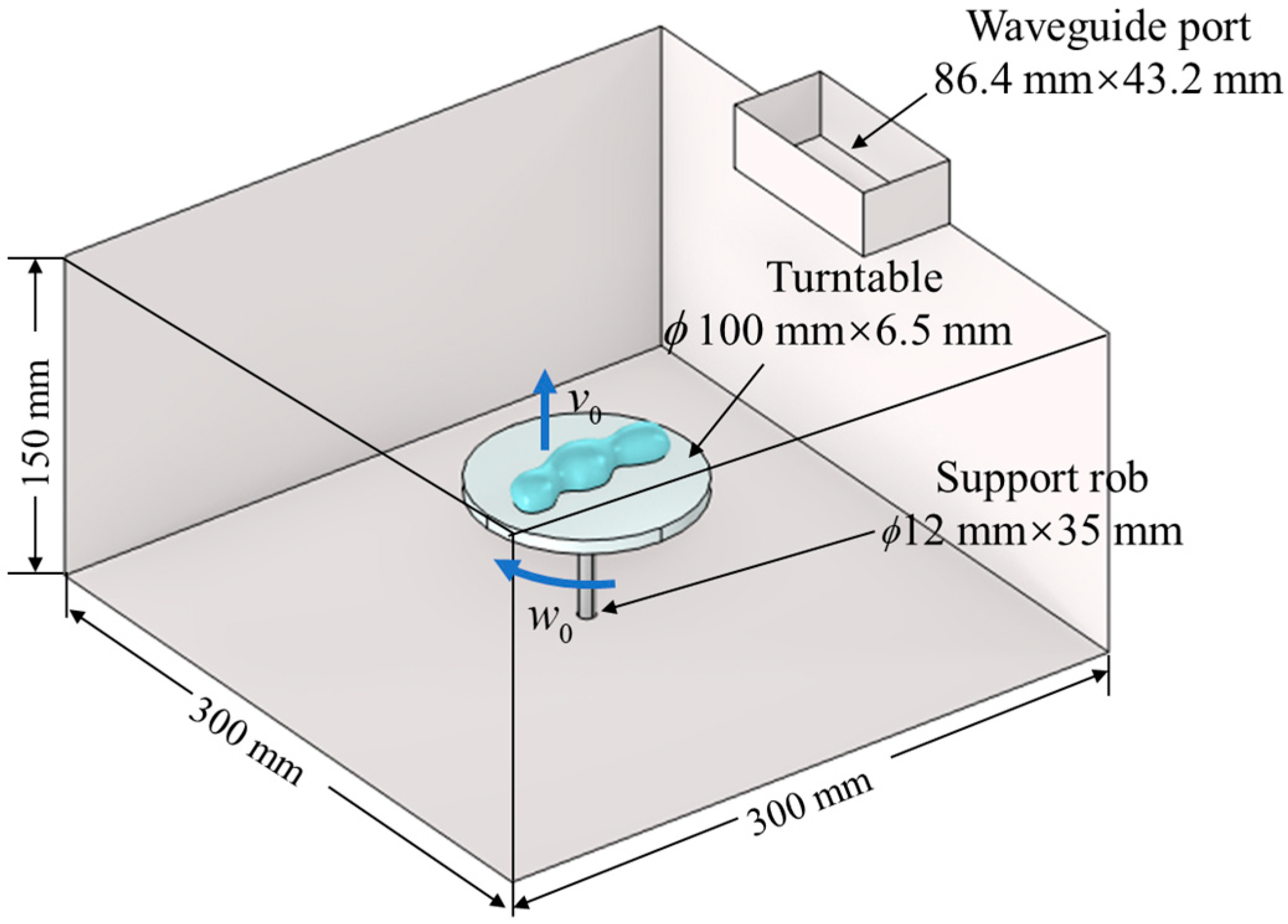
2.1. Simulation Model Geometry

In this paper, a three-dimensional microwave oven model was established using COMSOL Multiphysics software (COMSOL 6.3, Stockholm, Sweden). The geometric structure of the model is shown in Figure 1. The size of the microwave cavity is 300 mm × 300 mm × 150 mm, and there is a BJ26 waveguide on the top for microwave feeding. A quartz turntable with a diameter of 50 mm and a thickness of 6.5 mm is located at the center of the bottom of the rectangular cavity and is driven by a polyethylene rod with a diameter of 8 mm. It can rotate clockwise or counterclockwise and can also rise or fall. The heated sample is placed at the center of the turntable.

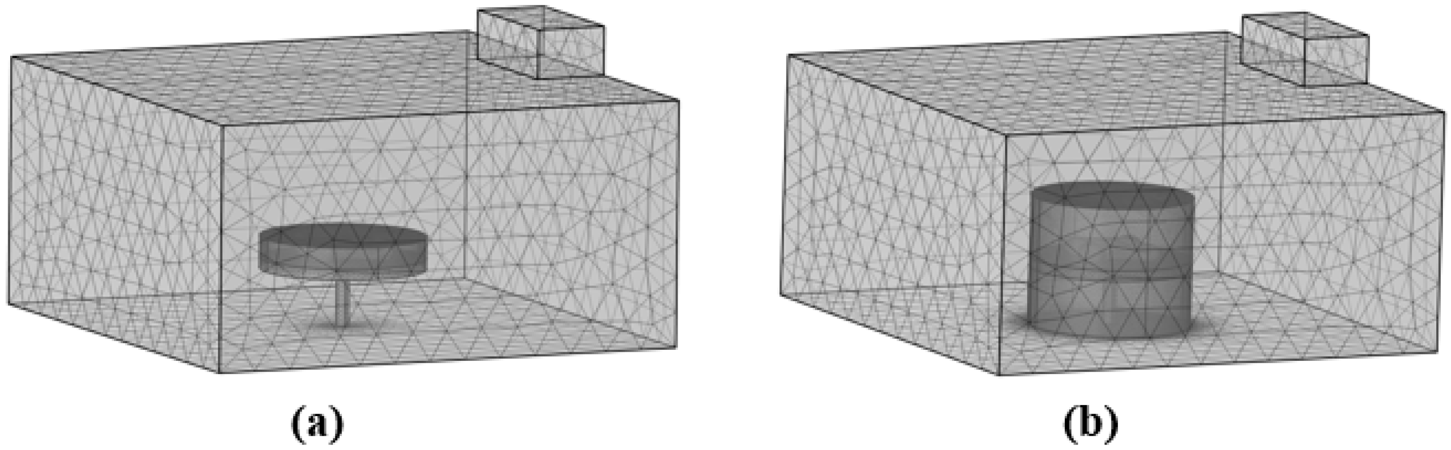
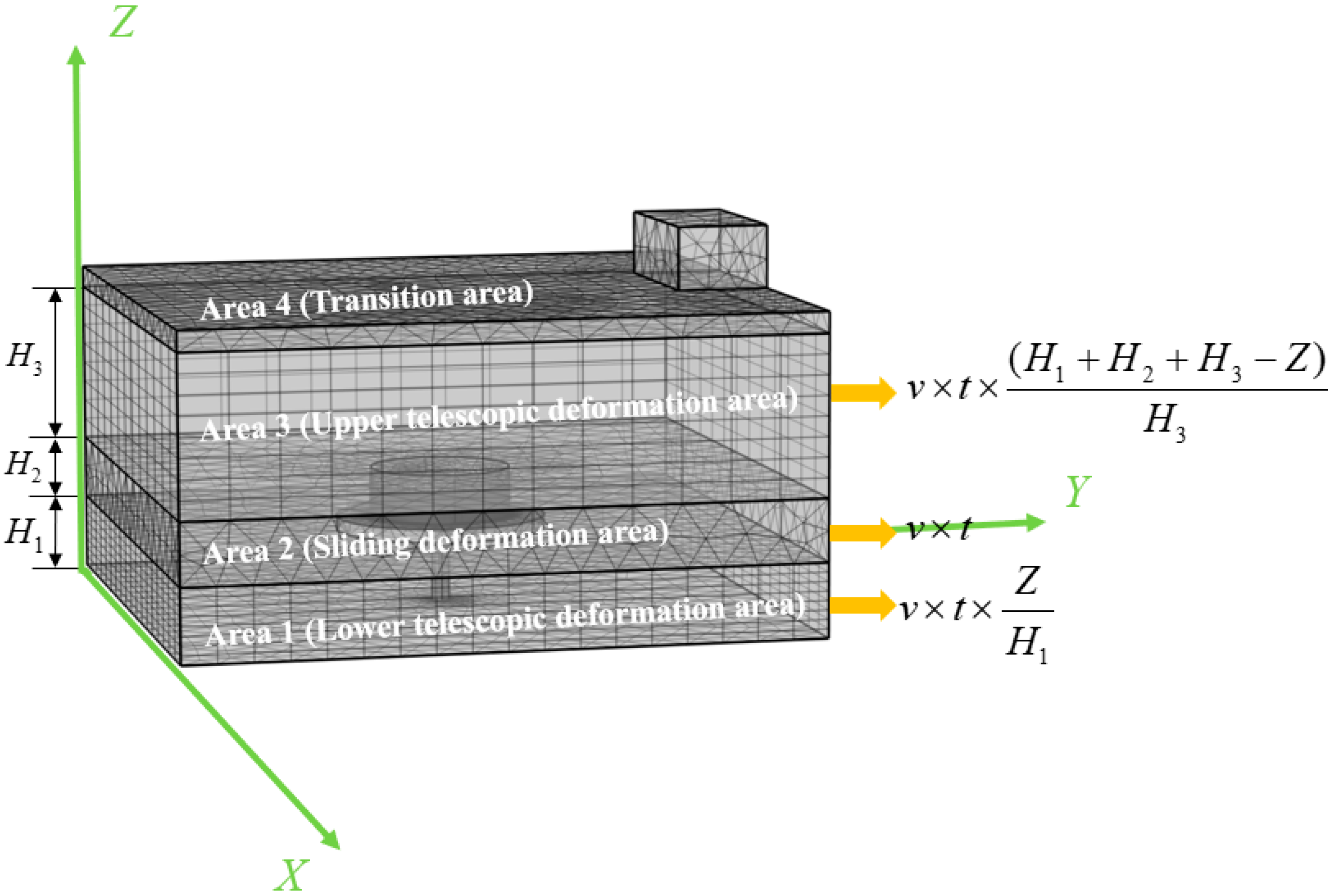
2.2. Design of Moving Mesh in Microwave Heating Calculation

In the implicit method, the mesh division of the sample in the rotating motion and the rotating with lifting motion are shown in Figure 2a and Figure 2b, respectively. It can be seen that, since the mesh of the lifting motion area needs to be refined in the rotating and lifting motion, the number of meshes increases rapidly with the increase in the sample movement distance. In order to improve the computational efficiency of the rotating and lifting motion, this study adopts the method of prescribed deformation of the moving mesh, which divides the mesh into two parts: the sliding mesh and the telescopic mesh. The sliding mesh generally divides the moving sample and its surrounding area into tetrahedral meshes. During the calculation process, the sliding mesh area moves as a whole, and the mesh structure remains relatively unchanged. In order to facilitate stretching and compression, the telescopic mesh generally divides the upper and lower parts of the sliding mesh into a swept mesh form.
The mesh division of the overall simulation model in this chapter is shown in Figure 3. It can be seen that the mesh area is divided into four layers, namely the lower telescopic deformation area (area 1), the sliding deformation area (area 2), the upper telescopic deformation area (area 3), and the transition area (area 4). Area 1 includes the lower cavity and the support rod. Since there is no interface change, the easily stretched swept mesh can be directly adopted. Area 2 includes both the tray and the sample to be heated, which needs to refine the mesh of the moving region of the sample to be heated, so as to perform the calculation of rotating motion in conjunction with the ray-casting method, and free tetrahedrons are used for mesh area 2. Area 3 is same as area 1, and can be directly divided in the form of a swept mesh. However, in the daily use of microwave ovens, the top surface may not be flat. As shown in Figure 3, there may be a feed on the top surface of the cavity, meaning that area 4 needs to be added to provide a consistent interface between areas 4 and area 3. Area 4 is meshed with free tetrahedrons, and the mesh in this area remains unchanged during the calculation. Therefore, the internal refined mesh only needs to include the rotating motion area in area 2, which greatly reduces the number of meshes and calculation time.
The meshes of the telescopic deformation area and the sliding deformation area change over time. The meshes in areas 1 and 3 will deform accordingly with different z-axis coordinates, and the mesh in area 2 will translate with the moving equation. For the rotating and lifting motion, the overall mesh deformation method is shown in Figure 3, where H1, H2, and H3 represent the height of area 1, area 2, and area 3 in the lifting direction at the initial time.
In this study, the sample undergoes a uniform rotating and lifting motion with a lifting speed v 0 . The deformation distance of area 1 at different z coordinates and time t during the lifting motion is shown as
D 1 ( z , t ) = v 0 t z H 1
where D 1 ( z , t ) is the function of the z coordinate and time. It can be seen that the mesh deformation distance is different for different z coordinates. The deformation distance of area 2 is:
D 2 ( t ) = v 0 t
The mesh in area 2 is uniformly displaced with no relative deformation. The deformation distance of area 3 is given by:
D 3 ( z , t ) = v 0 t ( H 1 + H 2 + H 3 z ) L 3
In area 1, when the z coordinate is 0, D 1 ( 0 ) is 0, indicating that the bottom of the cavity is fixed and will not deform. The z coordinate of the upper surface of region 1 is H1, D 1 ( H 1 ) is v 0 t , and the deformation distance of the top surface of area 1 is the same as the translation distance of area 2, such that the mesh of areas 2 and 1 will not be layered.
At the bottom of area 3, when z coordinate is H1 + H2, the D 3 ( H 1 + H 2 ) is v 0 t , and the deformation distance of the bottom of area 3 of the cavity can be consistent with the translation distance of area 2, meaning that the meshes of areas 2 and 3 will not be layered. At the top of area 3, when z coordinate is H1 + H2 + H3, the D 3 ( H 1 + H 2 + H 3 ) is 0, and no deformation will occur.
Figure 4a and Figure 4b show, respectively, the mesh distribution at the initial time and the final time. It can be seen that the meshes of areas 1 and 3 are stretched or compressed according to the position of the sample, and the mesh of area 2 where the sample is located has only changed position. At this time, the meshes are consistent at different time steps, and the area where the sample is located will also shift with the deformation of the mesh, thereby ensuring the accuracy of the calculation.

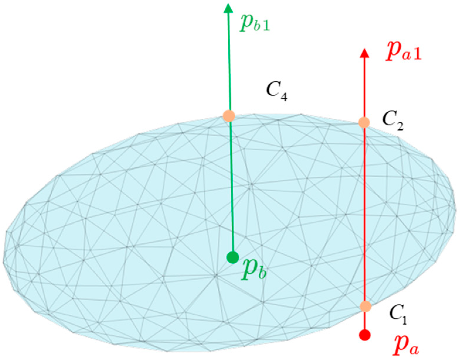
2.3. Representation of Sample in the Model

The moving mesh introduced in the model can only describe the lifting motion of the sample. When the sample rotates at the same time, the sample in the refined mesh moving region needs to be implicitly represented in area 2. The boundary recognition method based on the ray-casting method is to emit a ray at point p in order to determine whether point p is within the sample boundary by calculating the parity of the ray passing through the sample boundary [21].
N ( r p ) = 2 n 1 , n = 1 , 2 , p B o u n d a r y i n 2 n , n = 0 , 1 , p B o u n d a r y o u t
where N r p is the number of rays crossing the sample boundary. As shown in Figure 5, when N r p b is an even number, point pb is outside the boundary, and when N r p a is an odd number, point pa is inside the boundary. After the inside and outside identification, the Heaviside function is used to indicate whether the point is within the sample boundary.
H r p = 1 , i f r p B o u n d a r y i n 1 , i f r p B o u n d a r y 0 , o t h e r w i s e
The value is 1 when the point is inside or on the boundary; otherwise, it is outside the boundary.

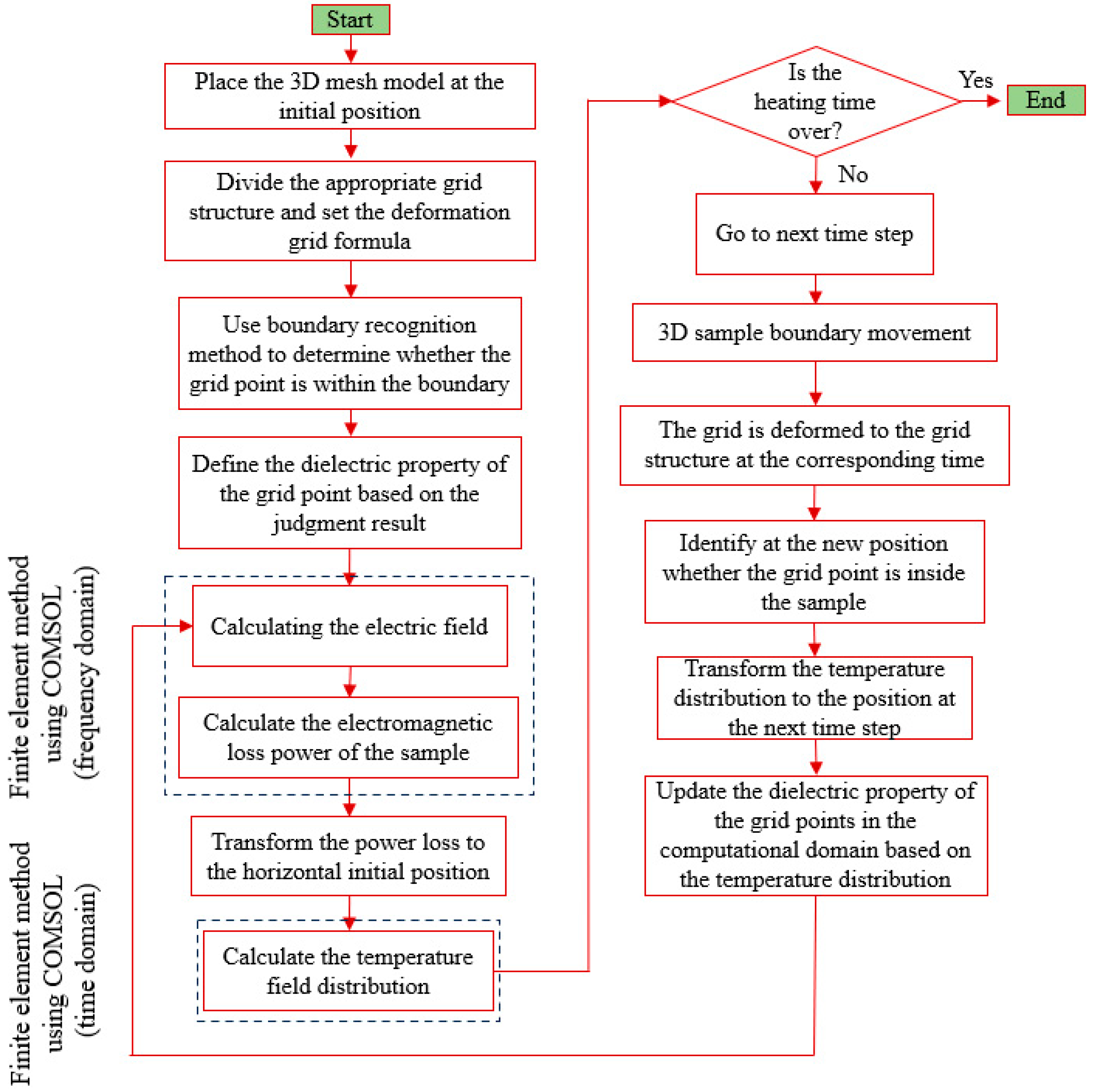
2.4. Microwave Heating Multi-Physics Simulation Process

In electromagnetic calculations, complex-shaped samples are implicitly represented by refined mesh. According to the Heaviside function results obtained by identifying inside and outside the boundary [28], we assign electromagnetic parameters to each mesh point in the moving region, as follows:
ε ( r , T ) = ε 2 ( T ) ( 1 H ( r ) ) + ε 1 ( T ) H ( r )
where ε 1 and ε 2 represent the relative permittivity of the sample and the material outside the sample, respectively, and T represents the temperature value. The relative permittivity value varies greatly with temperature and is set as a function of temperature and space.
In electromagnetic field simulation, the electromagnetic wave distribution in the cavity can be calculated by Maxwell’s wave equation. The distribution of relative permittivity and relative permeability in the equation determines the distribution of the field. We express the dielectric parameters of the wave equation as a function of space and temperature based on the identification results inside and outside the boundary and the temperature distribution in space, as shown below:
× μ 1 × E k 0 2 ε ( r , T ) j ε ( r , T ) E = 0
where μ represents the relative permeability of the material, E represents the electric field vector in space, k0 represents the propagation constant in vacuum, ε represents the real part of the relative permittivity, and ε represents the imaginary part of the relative permittivity. In the microwave heating calculation, the waveguide port corresponds to a BJ-26 rectangular waveguide that injects 100 W of 2.45 GHz microwave power into the cavity in the TE10 mode. The cavity wall is set as a perfect electrical conductor, and the tangential component of the electric field is zero, as follows:
n × E = 0
where n is the unit normal vector of the surface. The electromagnetic power loss generated when an electromagnetic wave passes through a lossy dielectric medium is used as a heat source in the temperature calculation process and is given by
Q e r , t = 1 2 ω ε 0 ε r , T | E | 2
where w represents the frequency of the electromagnetic wave. It can be seen that the electromagnetic dissipated power is a function of space and temperature.
Before calculating the temperature field at each time step, the heat source position needs to be transformed to the initial position in order to ensure the consistency of temperature inheritance. In the microwave heating multi-physics field calculation of the proposed method, the moving mesh is introduced. The z-axis position of the sample changes at different time steps. When calculating the temperature field during the rotating and lifting motion, only the rotating angle needs to be transformed to the initial position [29].
Q ( r ) θ 0 = Q ( r ) θ n m = 1 n w 0 ( m 1 ) Δ t
where Q ( r ) θ 0 represents the horizontal rotating angle of the sample at the initial time, and Q ( r ) θ n represents the rotating angle of the sample at the nth time step. The temperature distribution in the sample can be obtained by the heat conduction equation:
ρ C p T k T = Q e
where ρ represents the density of the sample to be heated, Cp is the specific heat capacity, k is the thermal conductivity, and Qe is the heat source generated by the electric field loss. In addition to the heat transfer inside the heated sample, the surface also exchanges heat with the surrounding air through thermal convection:
n q = h ( T T a i r )
where n is the unit normal vector, q is the heat flux, h is the heat transfer coefficient, and Tair is the temperature of the air. In this study, h is set to 10 W/(m2∙K), the initial temperature of the heated sample and the air is set to 20 °C. Considering the relatively short heating time, the thermal insulation boundary condition is set between the heated material and the tray.
The dielectric property of the sample to be heated changes greatly with temperature, and the relative permittivity of the sample needs to be updated according to the temperature distribution at each time step. Therefore, before performing electromagnetic calculations in the next time step, the temperature distribution of the sample needs to be converted to the actual position to update the relative permittivity
T ( r 0 , t n ) T ( r n + 1 , t n )
where T ( t n + 1 ) changes by Δ t time relative to T ( t n ) . The overall calculation flow chart is shown in Figure 6.

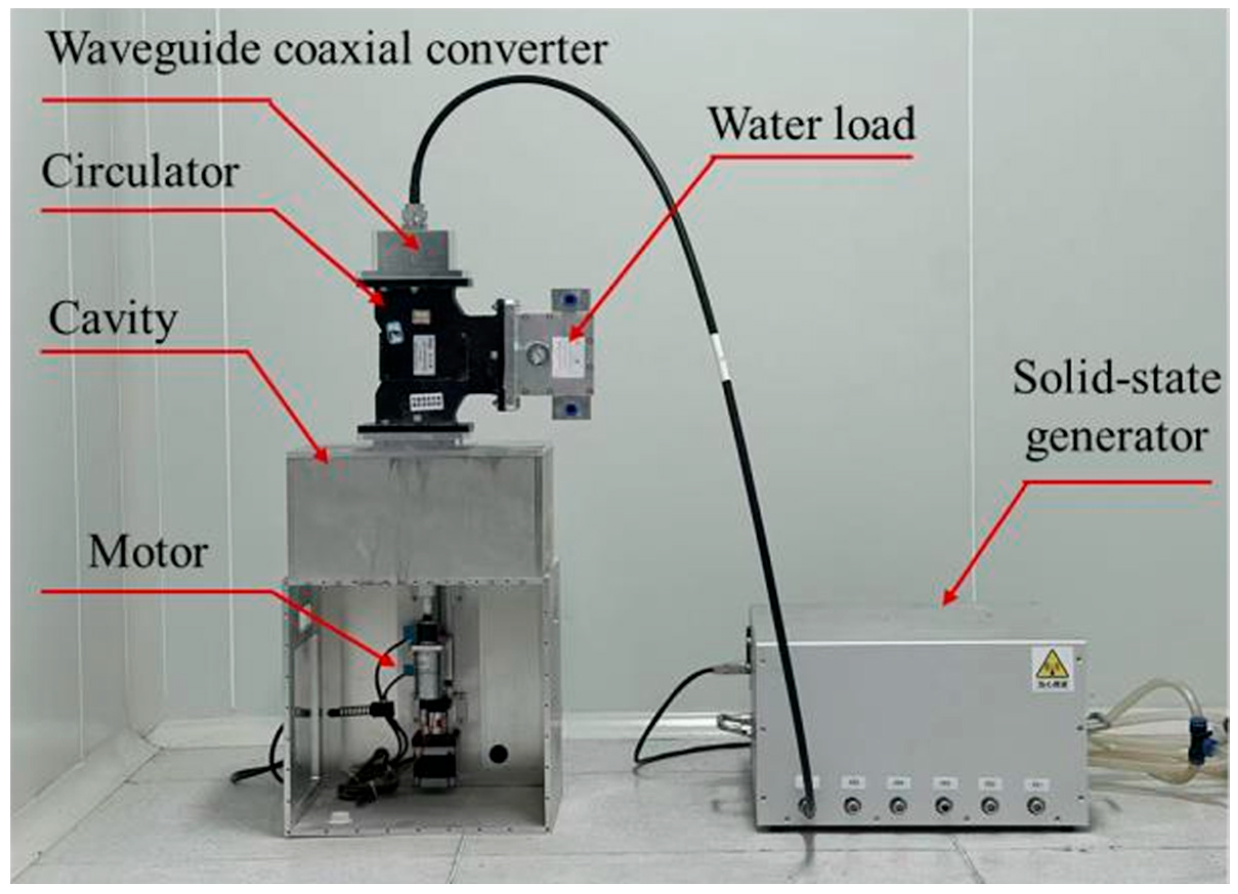
2.5. Experimental Settings

In order to verify the proposed method, an experimental system was built, as shown in Figure 7. Microwaves were fed into the cavity by a solid-state power generator (WSPS-2450-200M, Wattsine, Chengdu, China) through a waveguide coaxial connector, with an input power of 100 W at 2.45 GHz. A directional coupler and a microwave power meter (AV2433, the 41st Institute of China Electronic Technology Group Corporation, Anhui Province, China) were used to measure the effective feeding microwave power at 2.45 GHz. The circulator and water load were used to protect the solid-state power generator by absorbing the microwave energy reflected by the cavity. A motor was positioned under the cavity to drive the rotation of the turntable and the lifting of the support rod. After heating, a thermal imager (UTi160H) was used to record the surface temperature of the heated sample. The sample to be heated was placed in the center of the turntable, which was agar with a water content of 99.5%. The total time of the microwave heating process was 24 s, the lifting speed during the heating process was 1 mm/s, and the rotating velocity was π/12 rad/s. The relative permittivity of agar changes with temperature. The electromagnetic parameters and thermal parameters of the materials in the cavity are shown in Table 1.

3. Results and Discussion

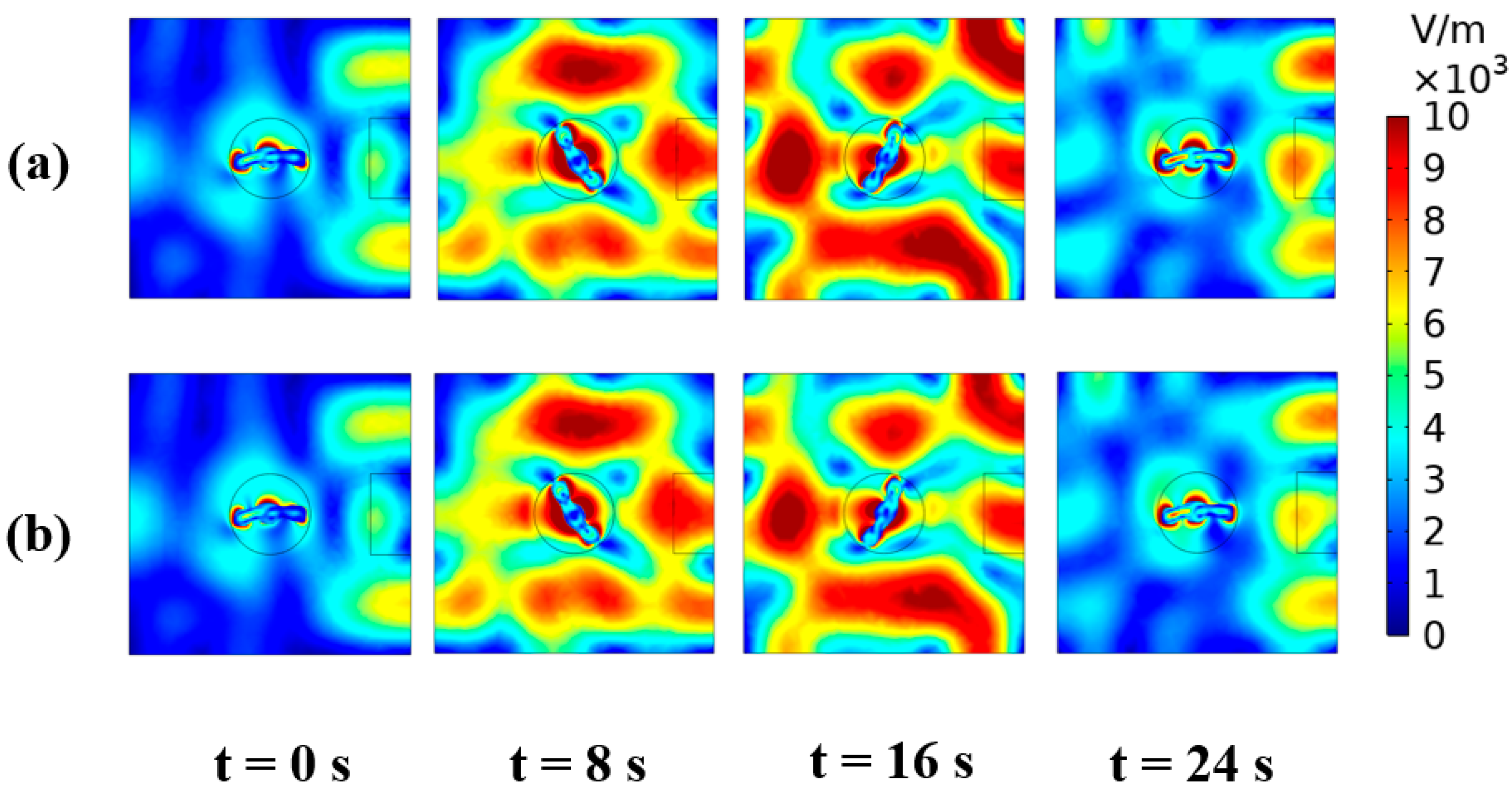
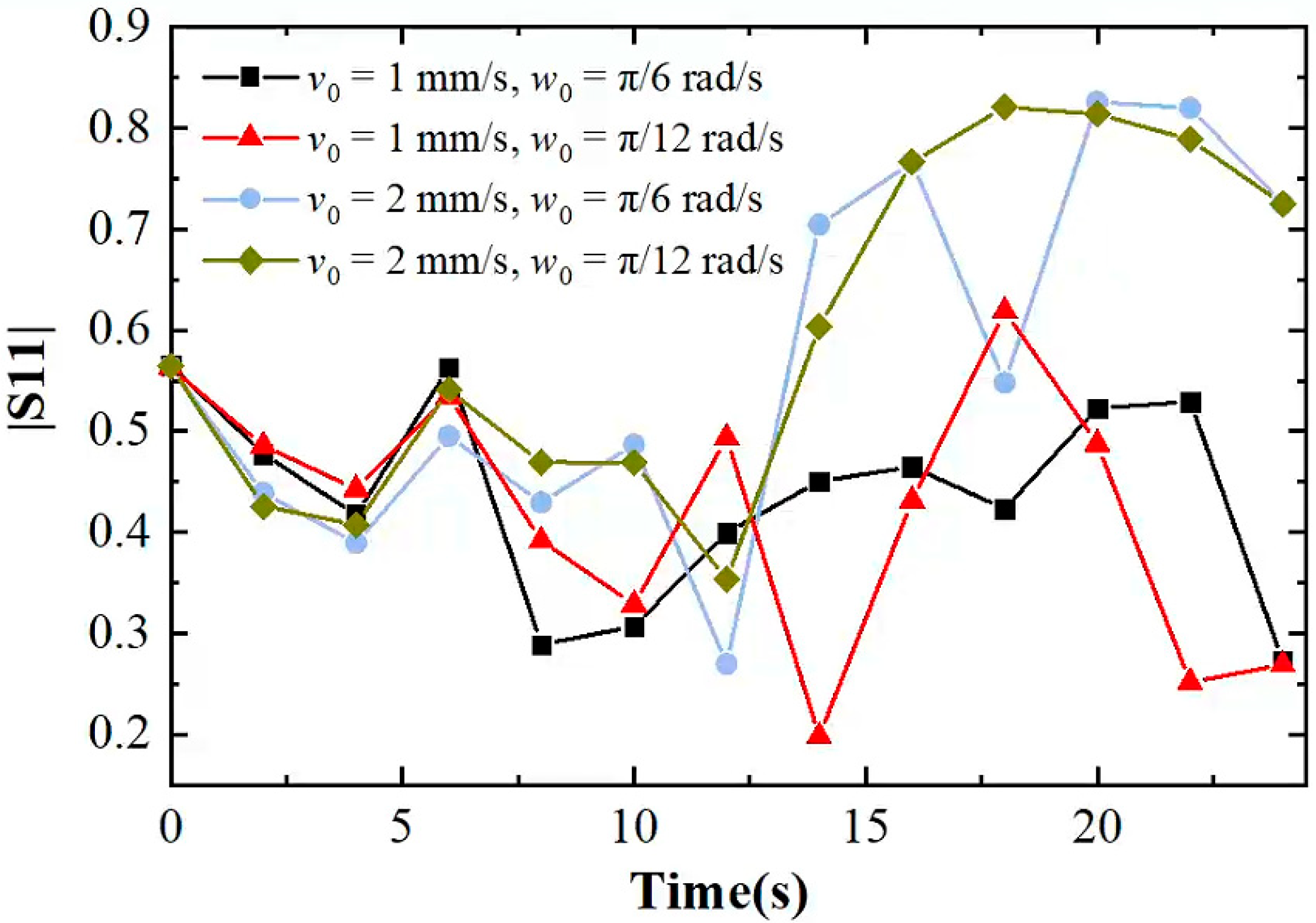
3.1. Validation of Electromagnetic Field Model

In order to verify the correctness of the proposed method in electromagnetic field calculations, a complex-shaped sample was selected to perform a rotating and lifting motion for calculation. Before the calculation, the mesh independence was studied by normalized power absorption (NPA). NPA is defined as the ratio of the average dissipated power absorbed by the lossy medium to the effective input power. If the change in the NPA value is less than 1%, it can be considered that the calculation result is independent of the mesh density. Figure 8 shows the relationship between NPA and the maximum mesh size in the refined mesh. Considering the calculation time and calculation accuracy, the maximum mesh size is 1.7 mm and the number of meshes is 490907 (386101 elements in the refined mesh). All the simulations were performed on the same workstation with 128 gb RAM running memory and an Intel® Xeon® Gold 5218 processor with a working frequency of 2.3 GHz.
First, the electromagnetic field calculation results obtained by the proposed method at different times were compared with the results obtained by the proposed method. As shown in Figure 9, it can be seen that the electric field distributions obtained by the two methods are consistent. The discrete method is intended to establish the geometric shape of the corresponding position of the sample movement before calculation. At the same time, the port reflection coefficient S11 calculated by the two methods at different times is shown in Figure 10. The results show that the S11 calculated by the proposed method is consistent with the S11 calculated by the discrete method, with a maximum error of only 0.05, which verifies the accuracy of the proposed method.

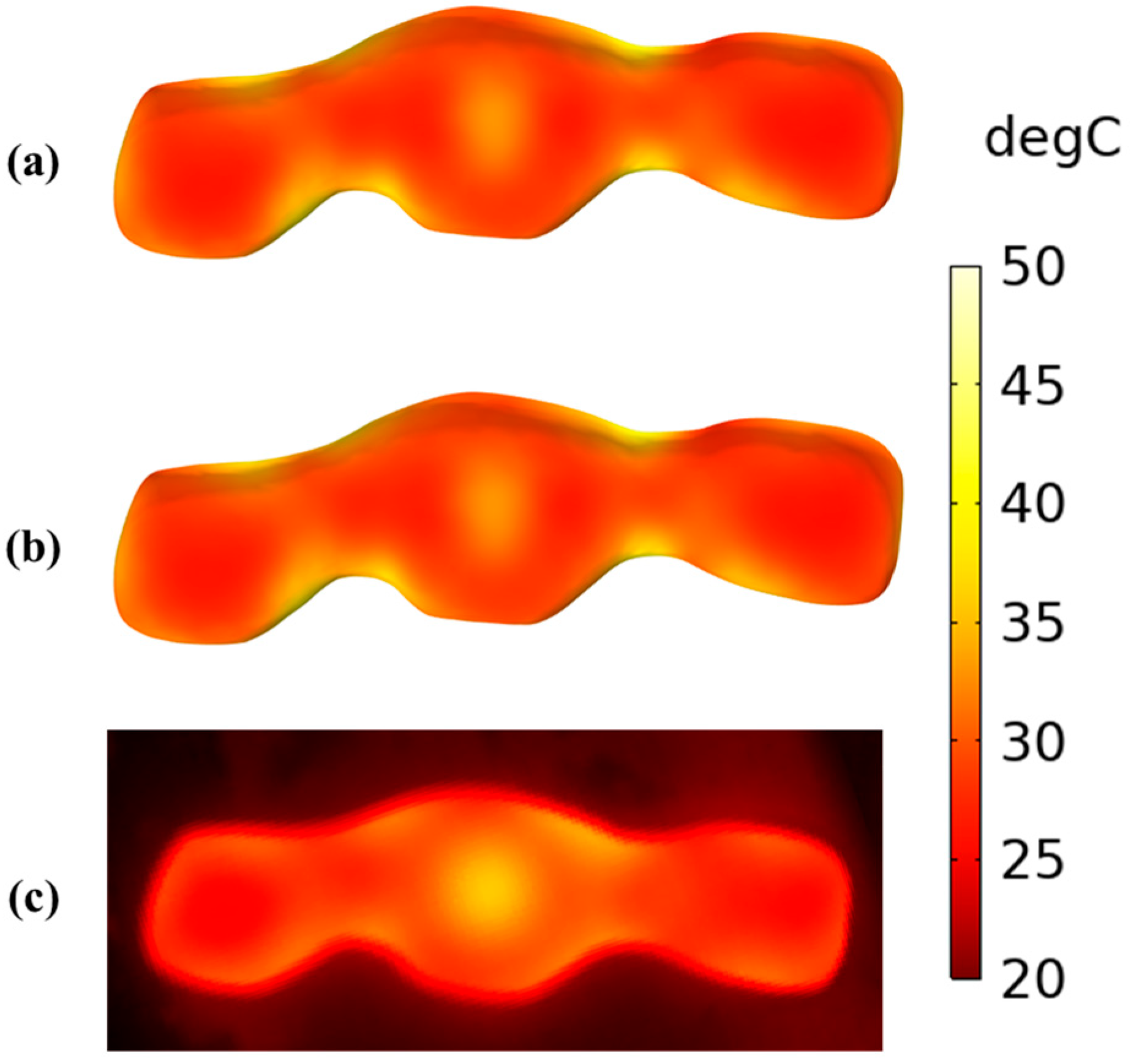
3.2. Temperature Distribution

Under the same mesh size of the moving region, the total number of meshes used in the simulation of the proposed method and the ray-casting method is 490,907 and 2,114,187, respectively. It can be seen that the number of meshes of the proposed method under large-scale motion is greatly reduced compared to the ray-casting method. The moving region mesh divided by the ray-casting method is a cylinder, which includes the motion area of the sample, while the moving region mesh divided by the proposed method in this paper only includes the area where the sample moves horizontally. The number of meshes and the calculation time of the two methods are shown in Table 2. It can be seen that the number of meshes of the method proposed in this paper has dropped to 23% of the original, and the time has dropped to 9.8%, which improves the calculation efficiency. The total computation time includes both frequency-domain and transient simulation phases. The total simulation time includes both frequency-domain and transient phases. The proposed method achieves a significant speed-up in the frequency-domain simulation (1.3 min vs. 17.9 min) thanks to its reduced mesh scale. In contrast, the transient-phase runtimes are nearly identical (~0.5 min) because both methods compute the same sample domain with the same mesh and solver settings.
During the experiment, a thermal imager was used to capture the temperature distribution on the sample surface. We compared the temperature distribution results calculated by the proposed method and the RCM with the experimental results, as shown in Figure 11. The initial temperature of the sample during the microwave heating simulation was 20 °C.
It can be seen that the temperature distribution results calculated by the proposed method are consistent with those calculated by the ray-casting method. The experimental surface temperature is slightly lower than the simulation temperature, but the overall temperature distribution is consistent with the simulated surface temperature distribution. The overall low temperature in the experiment is due to the fact that it takes a certain amount of time for the microwave source to reach the set power after it is turned on. There is a time interval of about 10 s between the end of sample heating and the capture of the thermal image of the sample surface, during which the heat of the sample will dissipate into the air. Another reason is that the sample thermal parameters used in the simulation are water, which is not set as a function of temperature, so there will be some errors compared with the actual heating situation.
In order to make a more accurate comparison, we used a fiber optic thermometer to measure the real-time temperature at the center of the sample and compare the measured temperature with the simulation results, as shown in Figure 12. The average error between the experimental instantaneous temperature at the center of the sample and the simulated instantaneous temperature is 2.5%, and the experimental results are consistent, which verifies the accuracy of the proposed method.

3.3. Effects of Rotating Speed and Lifting Speed on Heating Efficiency and Uniformity

In addition, the influence of different movement speeds of rotating and lifting on microwave heating performance was explored using this sample as an example. Temperature covariance (COV) is used to quantitatively analyze heating uniformity
C O V = 1 N i = 1 N T i T ¯ 2 / T ¯ T 0
where T i represents the temperature at different mesh points of the sample, N is the total number of the mesh points of the sample, and T ¯ represents the average temperature of the sample.
It can be observed from Table 3 and Figure 13 that different movement conditions have a relatively large influence on heating performance. When the lifting speed is the same, different rotating speeds w0 have little effect on the temperature distribution and heating efficiency (i.e., volume average temperature rise) of the sample. The heating efficiency at the lifting speed v0 = 1 mm/s is higher than that at the lifting speed v0 = 2 mm/s. This is because the energy reflection from the cavity increases as the sample rises, as shown in Figure 14. The COV value is relatively small when the lifting speed v0 = 2 mm/s. The change in the power dissipation distribution of the sample during heating increases with the increase in the vertical lifting distance, making the overall temperature distribution more uniform.

4. Conclusions

This study proposes a microwave heating calculation method for large-scale motion of complex-shaped samples, which can improve the calculation efficiency compared to previous methods. The method introduces the moving mesh for calculation, selects the appropriate moving mesh area, and divides the model into the stretching mesh deformation area and the sliding mesh deformation area. For the rotating and lifting motion, the telescopic deformation mesh is stretched or compressed at different times to eliminate the refined grid area caused by the lifting motion. Then, combined with a boundary recognition algorithm based on the ray-casting method, the electromagnetic parameters are assigned to each grid point, and the horizontal rotating motion is calculated while calculating the large-scale translation. By analyzing the microwave oven model with a rotating and lifting turntable, the maximum error of the reflection coefficient calculated by this method and the traditional discrete position method is 0.05, and the calculation time is reduced to 9.8% of the RCM, which verifies the efficiency and accuracy of the algorithm. At the same time, a microwave heating experiment of complex-shaped samples with rotating and lifting motion was designed. The experimental results show that the proposed method can accurately calculate the microwave heating process, and the average error of the sample center temperature is 2.5%. Finally, the effects of different lifting speeds and rotating speeds on sample heating uniformity and efficiency were discussed. This method can be used for microwave heating calculation of large-scale motion of complex-shaped samples, improving the calculation efficiency.

Author Contributions

Conceptualization, Y.H. and F.Y.; methodology, Y.H.; software, F.Y.; validation, Y.W., F.Y. and W.X.; formal analysis, F.Y.; investigation, Y.W. and W.X.; resources, L.D.; data curation, W.X.; writing—original draft preparation, Y.H. and L.D.; writing—review and editing, F.Y.; visualization, Y.H.; supervision, L.D.; project administration, F.Y.; funding acquisition, L.D. All authors have read and agreed to the published version of the manuscript.

Funding

This study was supported by the Sichuan Science and Technology Program under Grant No. 2024ZYD0263, the Key Project of Chengdu City under Grant No. 2024-JB00-00012-GX, the Shanxi Science and Technology Cooperation and Exchange Special Project under Grant No. 202204041101030, and the Shanxi Science and Technology Achievement Transformation–Guiding Special Project under Grant No. 202304021301044.

Data Availability Statement

Data are contained within the article.

Conflicts of Interest

Author Lu Dong was employed by the company Chengdu Micropower Tech Co., Ltd. The remaining authors declare that the research was conducted in the absence of any commercial or financial relationships that could be construed as a potential conflict of interest.

References

  1. Peng, Y.; Zhou, D.; Chen, H.; Liu, M.; Tang, Z.; Hong, T. Resonance-Driven Microwave Heating of Low-Loss Cylindrical Substances in Waveguide Systems. IEEE Trans. Microw. Theory Tech. 2024, 72, 3722–3733. [Google Scholar] [CrossRef]
  2. Yin, C. Microwave-Assisted Pyrolysis of Biomass for Liquid Biofuels Production. Bioresour. Technol. 2012, 120, 273–284. [Google Scholar] [CrossRef] [PubMed]
  3. Kappe, C.O.; Stadler, A.; Dallinger, D. Microwaves in Organic and Medicinal Chemistry; John Wiley and Sons: Hoboken, NJ, USA, 2012. [Google Scholar]
  4. Chandrasekaran, S.; Ramanathan, S.; Basak, T. Microwave Food Processing—A Review. Food Res. Int. 2013, 52, 243–261. [Google Scholar] [CrossRef]
  5. Liu, M.; Zhou, D.; Peng, Y.; Tang, Z.; Huang, K.; Hong, T. High-Efficiency Continuous-Flow Microwave Heating System Based on Metal-Ring Resonant Structure. Innov. Food Sci. Emerg. Technol. 2023, 85, 103330. [Google Scholar] [CrossRef]
  6. Tang, J.; Hao, F.; Lau, M. Microwave Heating in Food Processing. In Advances in Bioprocessing Engineering; Springer: Dordrecht, The Netherlands, 2002; pp. 1–44. [Google Scholar]
  7. Ye, J.; Lan, J.; Xia, Y.; Yang, Y.; Zhu, H.; Huang, K. An Approach for Simulating the Microwave Heating Process with a Slow-Rotating Sample and a Fast-Rotating Mode Stirrer. Int. J. Heat Mass Transf. 2019, 140, 440–452. [Google Scholar] [CrossRef]
  8. Kurniawan, H.; Alapati, S.; Che, W.S. Effect of Mode Stirrers in a Multimode Microwave-Heating Applicator with the Conveyor Belt. Int. J. Precis. Eng. Manuf.-Green Technol. 2015, 2, 31–36. [Google Scholar] [CrossRef]
  9. Chen, J.; Pitchai, K.; Birla, S.; Jones, D.D.; Subbiah, J. Modeling Heat and Mass Transport during Microwave Heating of Frozen Food Rotating on a Turntable. Food Bioprod. Process. 2016, 99, 116–127. [Google Scholar] [CrossRef]
  10. Wang, L.; Yang, Y.; Zhang, Y.; Tang, J. Modeling the RF Heating Uniformity Contributed by a Rotating Turntable. J. Food Eng. 2023, 339, 111289. [Google Scholar] [CrossRef]
  11. Rodriguez, J.; Morona, L.; Erans, M.; Buttress, A.J.; Nicholls, M.; Batchelor, A.R.; Duran-Jimenez, G.; Kingman, S.; Groszek, D.; Dodds, S. Solving the microwave heating uniformity conundrum for scalable high-temperature processes via a toroidal fluidised-bed reactor. Chem. Eng. Process.-Process Intensif. 2024, 202, 109838. [Google Scholar] [CrossRef]
  12. Bae, S.-H.; Jeong, M.-G.; Kim, J.-H.; Lee, W.-S. A Continuous Power-Controlled Microwave Belt Drier Improving Heating Uniformity. IEEE Microw. Wirel. Compon. Lett. 2017, 27, 527–529. [Google Scholar] [CrossRef]
  13. Yi, Q.; Lan, J.; Ye, J.; Zhu, H.; Yang, Y.; Wu, Y.; Huang, K. A Simulation Method of Coupled Model for a Microwave Heating Process with Multiple Moving Elements. Chem. Eng. Sci. 2021, 231, 116339. [Google Scholar] [CrossRef]
  14. Geedipalli, S.S.R.; Rakesh, V.; Datta, A.K. Modeling the Heating Uniformity Contributed by a Rotating Turntable in Microwave Ovens. J. Food Eng. 2007, 82, 359–368. [Google Scholar] [CrossRef]
  15. Pitchai, K.; Chen, J.; Birla, S.; Gonzalez, R.; Subbiah, J. A Microwave Heat Transfer Model for a Rotating Multi-Component Meal in a Domestic Oven: Development and Validation. J. Food Eng. 2014, 128, 60–71. [Google Scholar] [CrossRef]
  16. Zhu, H.-C.; Liao, Y.-H.; Xiao, W.; Ye, J.-H.; Huang, K.-M. Transformation Optics for Computing Heating Process in Microwave Applicators with Moving Elements. IEEE Trans. Microw. Theory Tech. 2017, 65, 1434–1442. [Google Scholar] [CrossRef]
  17. Lian, C.; Li, J.-J.; Zhang, Y.; Ye, J.-H.; Zhu, H.-C.; Huang, K.-M. A General Inheritance Algorithm for Calculating of Arbitrary Moving Samples during Microwave Heating. IEEE Trans. Microw. Theory Tech. 2022, 70, 1964–1974. [Google Scholar] [CrossRef]
  18. Ye, J.-H.; Zhu, H.-C.; Liao, Y.-H.; Xiao, W.; Huang, K.-M. Implicit Function and Level Set Methods for Computation of Moving Elements during Microwave Heating. IEEE Trans. Microw. Theory Tech. 2017, 65, 4773–4784. [Google Scholar] [CrossRef]
  19. Zhang, M.; Jia, X.; Tang, Z.; Li, Y.; Wang, Y. A Fast and Accurate Method for Computing the Microwave Heating of Moving Objects. Appl. Sci. 2020, 10, 2985. [Google Scholar] [CrossRef]
  20. Li, R.; Hong, T.; Liu, R.; Chen, H.; Yang, Y.; Zhu, H. Microwave Heating Multiphysics Computation of Moving Complex-Shaped Samples Based on Ray Casting Method. IEEE Trans. Microw. Theory Tech. 2024, 72, 1234–1245. [Google Scholar] [CrossRef]
  21. Ye, J.; Xu, C.; Zhang, C.; Zhu, H.; Huang, K.; Li, Q.; Wang, J.; Zhou, L.; Wu, Y. A Hybrid ALE/Implicit Function Method for Simulating Microwave Heating with Rotating Objects of Arbitrary Shape. J. Food Eng. 2021, 302, 110551. [Google Scholar] [CrossRef]
  22. Farag, K.W.; Lyng, J.G.; Morgan, D.J.; Cronin, D.A. A Comparison of Conventional and Radio Frequency Thawing of Beef Meats: Effects on Product Temperature Distribution. Food Bioprocess Technol. 2011, 4, 1128–1136. [Google Scholar] [CrossRef]
  23. Ye, J.; Zhu, H.; Lan, J.; Xia, Y.; Yang, Y.; Huang, K. Dynamic Analysis of a Continuous-Flow Microwave-Assisted Screw Propeller System for Biodiesel Production. Chem. Eng. Sci. 2019, 202, 146–156. [Google Scholar] [CrossRef]
  24. Tezduyar, T.E. Finite element methods for flow problems with moving boundaries and interfaces. Arch. Comput. Methods Eng. 2001, 8, 83–130. [Google Scholar] [CrossRef]
  25. Teixeira, P.R.F.; Awruch, A.M. Numerical Simulation of Fluid–Structure Interaction Using the Finite Element Method. Comput. Fluids 2005, 34, 249–273. [Google Scholar] [CrossRef]
  26. Küttler, U.; Wall, W.A. Fluid-Structure Interactions Using Different Mesh Motion Techniques. Comput. Struct. 2008, 86, 1523–1532. [Google Scholar]
  27. Gu, B.; Yang, C. A Review of the Computational Investigation of Three-Dimensional Transient Magneto-Thermal Coupling Characteristics of Electromagnetic Railgun Armature and Rail in High-Speed Sliding Electrical Contact. J. Phys. Conf. Ser. 2023, 2478, 082007. [Google Scholar] [CrossRef]
  28. Zhou, J.; Yang, X.; Chu, Y.; Li, X.; Yuan, J. A Novel Algorithm Approach for Rapid Simulated Microwave Heating of Food Moving on a Conveyor Belt. J. Food Eng. 2020, 282, 110029. [Google Scholar] [CrossRef]
  29. Roth, S.D. Ray Casting for Modeling Solids. Comput. Graph. Image Process. 1982, 18, 109–144. [Google Scholar] [CrossRef]
  30. Purcell, T.J.; Buck, I.; Mark, W.R.; Hanrahan, P. Ray Tracing on Programmable Graphics Hardware. In ACM SIGGRAPH 2005 Courses; ACM: Los Angeles, CA, USA, 2005. [Google Scholar]
  31. Rossi, S.; Benaglia, M.; Brenna, D.; Porta, R.; Orlandi, M. Three Dimensional (3D) Printing: A Straightforward, User-Friendly Protocol to Convert Virtual Chemical Models to Real-Life Objects. J. Chem. Educ. 2015, 92, 1398–1401. [Google Scholar] [CrossRef]
Figure 1. Model schematic.
Processes 13 02109 g001
Figure 2. Meshing of the rotating motion and the rotating and lifting motion based on the ray-casting method. (a) Meshing of rotating motion; (b) Meshing of the rotating with lifting motion.
Processes 13 02109 g002
Figure 3. Mesh division and deformation.
Processes 13 02109 g003
Figure 4. (a) Mesh distribution at the initial time; (b) Mesh distribution at the final time.
Processes 13 02109 g004
Figure 5. Schematic diagram of ray-casting.
Processes 13 02109 g005
Figure 6. Overall calculation flow chart.
Processes 13 02109 g006
Figure 7. Experimental system.
Processes 13 02109 g007
Figure 8. Variation of normalized power absorption (NPA) with maximum grid size.
Processes 13 02109 g008
Figure 9. Electric field comparison. (a) Discrete position method; (b) Proposed method.
Processes 13 02109 g009
Figure 10. S11 at different times calculated by two methods.
Processes 13 02109 g010
Figure 11. Temperature distribution obtained by two methods and experiments. (a) The RCM; (b) Proposed method; (c) Experimental results. (Unit: °C).
Processes 13 02109 g011
Figure 12. Temperature curve of the center point of the simulation experiment.
Processes 13 02109 g012
Figure 13. Temperature distribution after heating for 24 s under different motion conditions (a) v0 = 1 mm/s, w0  = π/6 rad/s, (b) v0 = 1 mm/s, w0 = π/12 rad/s, (c) v0 = 2 mm/s, w0 = π/6 rad/s, (d) v0 = 2 mm/s, w0 = π/12 rad/s.
Processes 13 02109 g013
Figure 14. |S11| for 24 s under different motion conditions.
Processes 13 02109 g014
Table 1. Material Parameters.
PropertyPhysical
Domains
ValueSource
Relative permittivityAgar ε = ε ( T ) j ε ( T ) [20]
Air1
Turntable4.2[30]
Support rod2.3[31]
Density   ( k g / m 3 )Agar1000[28]
Thermal conductivity
( W / m 3 K )
Agar0.609
Specific heat Capacity
( J / k g K )
Agar4190
Table 2. Mesh numbers and computation time of the two methods.
RCMProposed Method
Total number of meshes2,114,187490,907
Calculation time221 min21.6 min
Table 3. Average temperature rise T and COV values after 24 s of heating under different motion conditions.
v0 = 1 mm/s,
w0 = π/6 rad/s
v0 = 1 mm/s,
w0 = π/12 rad/s
v0 = 2 mm/s,
w0 = π/6 rad/s
v0 = 2 mm/s,
w0 = π/12 rad/s
COV0.4230.4240.40.36
T (°C)17.1116.7413.1511.95
Disclaimer/Publisher’s Note: The statements, opinions and data contained in all publications are solely those of the individual author(s) and contributor(s) and not of MDPI and/or the editor(s). MDPI and/or the editor(s) disclaim responsibility for any injury to people or property resulting from any ideas, methods, instructions or products referred to in the content.

