A Novel ARX-Based Approach for the Steady-State Identification Analysis of Industrial Depropanizer Column Datasets

Abstract

This paper introduces a novel steady-state identification (SSI) method based on the auto-regressive model with exogenous inputs (ARX). This method allows the SSI with reduced tuning by analyzing the identifiability properties of the system. In particular, the singularity of the model matrices is used as an index for steady-state determination. In this contribution, the novel SSI method is compared to other available techniques, namely the F-like test, wavelet transform and a polynomial-based approach. These methods are implemented for SSI of three different case studies. In the first case, a simulated dataset is used for calibrating the output-based SSI methods. The second case corresponds to a literature nonlinear continuous stirred-tank reactor (CSTR) example running at different steady states in which the ARX-based approach is tuned with the available input-output data. Finally, an industrial case with real data of a depropanizer column from PETROBRAS S.A. considering different pieces of equipment is analyzed. The results for a reflux drum case indicate that the wavelet and the F-like test can satisfactorily detect the steady-state periods after careful tuning and when respecting their hypothesis, i.e., smooth data for the wavelet method and the presence of variance in the data for the F-like test. Through a heat exchanger case with different measurement frequencies, we demonstrate the advantages of using the ARX-based method over the other techniques, which include the aspect of online implementation.

1. Introduction

Steady-state identification (SSI) methods allow the determination of when the process has attained its stationary operation. There are several reasons for the need for SSI methods. For example, phenomenological models that are used for online implementation of process systems frameworks, such as model predictive control (MPC) and real-time optimization (RTO), are typically based on lumped parameters that contain phenomena information embedded in their values [1]. For optimal performance, these parameters must be updated in order to maintain the actual representation of the system. These updates can be performed by periodically defining stationary models that represent a detected steady state. Without SSI, RTO for example, would define targets that characterize suboptimal process operation. Several issues and challenges for SSI methods have been pointed out in the literature [2,3], for instance multiple oscillations, irregular process data, errors of Types I and II and multiple parameters to be tuned or defined by the selected technique. In this work, a novel ARX-based approach is proposed and compared to selected SSI methods from the literature via different process examples, including an industrial system.

In the literature, SSI has gained the attention of considerable research in the last few decades. Cao and Rhinehart [4] proposed a methodology, denoted as the F-like test, based on the comparison of two variances for the determination of steady states with efficient computational time. Cao and Rhinehart [5] and Shrowti et al. [6] showed that tuning the critical values of the F-like test can improve the performance of the method. In addition, this technique has been tested for validation on different chemical processes, such as a pilot-scale two-phase flow experiment [7,8] and a fractional distillation unit [9]. Brown and Rhinehart [10] extended the F-like test to address the multivariable case in which a pilot-scale distillation process is used. Other implementations of the F-like test found in the literature correspond to its use as a stop criterion for neural networks [11] and as a convergence indicator for the optimization of stochastic models [12]. Bhat and Saraf [13] also expanded the F-like test to consider the early determination of steady states and gross error detection in a crude distillation unit by means of tuning the critical values, implementing a linear Kalman filter and performing data reconciliation by least-squares techniques. Kim et al. [14] used a moving window of data and its standard deviations for the determination of steady states in a vapor compression system. Kelly and Hedengren [15] developed a method for SSI, which depends on the tuning of the window size and the critical value of its index, to detect non-stationary drifts in chemical processes. Flehmig and Marquardt [16] reported a technique that can infer trends in unmeasured states by using a linear process model that relates the unmeasured and measured states. Even when the model is necessary in the above method, the authors discarded the use of nonlinear state estimation due to its computational cost and mention the benefits of this technique for monitoring and control. Jiang et al. [17] applied a wavelet methodology to a crude oil distillation, where experimental data were treated in order to extract valuable information from the process. In a separate effort, Jiang and coworkers [18] derived a method that detects steady-state points employing wavelet theory. In a brief overview, this approach is comprised of four steps: obtain the first derivative of the smoothed signal; filter the steady-state data; identify the steady-state period; and tune the threshold values. The above method has been applied to a crude oil unit and a recausticizing plant of a chemical pulp mill. Furthermore, the authors reported that the computational cost was not a problem, as the approach could be executed once per second. Korbel et al. [19] presented an approach for SSI for online applications by a combination of wavelet and statistical techniques. This method was applied to a paper machine and large-scale processes for steady-state detection in real time. Yao and coworkers [20] implemented an SSI methodology based on principal component analysis specific for batch processes, in which the Mahalanobis distance, the eigenvalue information, among others steps, were used in the proposed method. Finally, Le Roux et al. [21] and Tao et al. [22] proposed a technique based on a polynomial equation assuming a specified degree and a moving window of data. Such techniques were employed for SSI by using the polynomial slope as the index or critical value.

This paper contributes with a novel framework for the identification of steady states using an ARX model. Specifically, the index of this new method is defined based on the identifiability information obtained from the ARX model, in which the singularity of the process model indicates the steady-state condition. Thus, as a differential from the other methods mentioned above, the ARX-based approach considers the process model characteristics when defining its index. Simulated and industrial systems are used for the purpose of performance comparison among different SSI methods. A simulated dataset and a nonlinear continuous stirred-tank reactor (CSTR) (described in Pannocchia and Rawlings [23]) represent the theoretical cases. The other key contribution of this paper lies in the implementation of the SSI methods to address a depropanizer column from PETROBRAS S.A., in which real industrial data are analyzed. The following techniques are applied to the case studies: the F-like test [4], the polynomial-based approach [22], the wavelet method [18] and the proposed ARX-based framework. In each of these techniques, tests are proposed to help guide the user decision on whether the system considered is at the steady state or not. Due to the statistical nature of the tests and the process noise patterns, such tests identify probable steady-state or transient conditions. The rest of this work is organized into four sections as follows. First, the SSI techniques are presented in Section 2. Then, the systems employed for the case studies are described. Later, the discussion of the results is shown in Section 4. Finally, the paper is closed with conclusions and future directions.

2. Steady-State Identification Techniques

In the following subsections, we present the four addressed steady-state identification techniques, which range from the classical to novel ones.

2.1. F-Like Test

Cao and Rhinehart [4] developed a method based on an F-like test. This method is widely used in the literature, especially due to its fast computational capabilities. These features are needed for online implementation, when SSI has to be combined with other computationally expensive techniques, such as MPC and RTO. Simply stated, this approach compares the ratio of two different estimated variances following the steps:

• A filtering value is estimated from the data:

  $$X_{f,1}={\lambda }_1{X}_i+(1-{\lambda }_1)X_{f,i-1}$$

  (1)

  where X is the process variable, X_f is the filtered value of X, λ₁ is a filter factor and i is the time sampling index.
• The initial variances are calculated by the following exponentially weighted moving average:

  $$v_{f,i}^2={\lambda }_2{\left(X_i-X_{f,i-1}\right)}^2+(1-{\lambda }_2)v_{f,i-1}^2$$

  (2)

  in which $v_{f,i}^2$ is the filtered value of a measure of variance based on the difference between process data and filtered values. Furthermore, $v_{f,i-1}^2$ is the previous variance filtered value, and λ₂ is a filter factor for the variance.
• The second filtered variance estimate is computed as:

  $${\delta }_{f,i}^2={\lambda }_3{\left(X_i-X_{i-1}\right)}^2+(1-{\lambda }_3){\delta }_{f,i-1}^2$$

  (3)

  where, once again, ${\delta }_{f,i}^2$ is the filtered value of a measure of variance based on the difference between data at different time units, ${\delta }_{f,i-1}^2$ is the previous filtered value and λ₃ is another filter factor for the variance.
• The ratio based on the two variances corresponds to the SSI index and is obtained by the following equation:

  $$R=\frac{(2-{\lambda }_1)v_{f,i}^2}{({\delta }_{f,i}^2)}$$

  (4)

In order to determine if the system is at steady state, the value of R is compared to a critical value, which corresponds to another parameter to be tuned. If R is greater than this critical value, the system is in transient behavior. Cao and Rhinehart [4] suggested the following filter factors for the best balance between errors of Type I and Type II (i.e., rejecting the null hypothesis when it is true and accepting it when it is false, respectively): λ₁ = 0.2, λ₂ = λ₃ = 0.1. The work in [4] also identified possible process issues that can affect R.

2.2. Adaptive Polynomial

Tao et al. [22] proposed a technique for steady-state identification that fits a polynomial of order two to a window of data. This window has a constant size and moves along with the process data. As in the previous technique, an index is defined for the determination of the steady-state condition.

For this method, a generic polynomial of order two is specified as follows:

$$x(t)=p_0+p_{1}t+p_2{t}^2$$

(5)

Furthermore, the vector of parameters to be estimated is expressed as:

$$\varphi =\left[p_0,p_1,p_2\right]$$

(6)

Additionally, the vector of regression variables is given by:

$$r(t)={\left[t^0,t^1,t^2\right]}^T$$

(7)

Using this vector, the polynomial above can be represented, as well, as:

$$x(t)={\varphi }^{T}r(t)$$

(8)

In order to determine the parameters of the polynomial for a window of size N, the following equation is solved:

$$\tilde{\varphi }={\left(R^{T}R\right)}^{-1}\tilde{x}$$

(9)

with:

$$R=\left[\begin{array}{c}r(1)\\ \cdot \\ \cdot \\ r(N)\end{array}\right]\tilde{x}=\left[\begin{array}{c}\tilde{x}(1)\\ \cdot \\ \cdot \\ \tilde{x}(N)\end{array}\right]$$

Finally, the index for this technique is defined by the following equation, as reported in the original paper:

$$|p_1|<\lambda ;\lambda =\frac{3\sigma }{N}$$

(10)

in which σ is the standard deviation. In this case, the parameter p₁ is used as an indicator of the steady-state condition. The only parameter to be tuned in this technique is the size of the window.

2.3. Wavelet-Based Method

This method that is based on the wavelet transform is taken from Jiang et al. [18]. As briefly mentioned above, this technique is comprised of the steps detailed below.

First, the acquired measurements need to be filtered to a certain degree by a user selected method. Then, the first and the second derivatives of the filtered data, d₁ and d₂, respectively, are calculated. In this work, we employ the “diff” function of MATLAB for that purpose. The thresholds T_s, T_w and T_u are computed by:

$$T_s={\sigma }_{d_1};T_w=\overline{d_1};T_u=3T_s\lambda$$

(11)

where λ is a tuning parameter, ${\sigma }_{d_1}$ is the standard deviation with respect to d₁ and $\overline{d_1}$ is the median of d₁.

Then, γ, θ(t) and ξ(θ(t)) are calculated as follows:

$$\gamma =\{\begin{array}{ll}0\hfill & \left|d_2\right|\le T_w\hfill \\ (\left|d_2\right|-T_w)/2T_w\hfill & T_w<\left|d_2\right|\hfill \\ 1\hfill & \left|d_2\right|\ge 3T_w\hfill \end{array}$$

(12)

$$\theta (t)=\left|d_1\right|+\gamma \left|d_2\right|$$

(13)

$$\xi (\theta (t))=1/2[\cos (\frac{\theta (t)-T_s}{T_u-T_s}\pi )+1]$$

(14)

The SSI index for this method is obtained as reported in the original paper by:

$$R_i=\{\begin{array}{ll}0\hfill & \theta (t)\ge T_u\hfill \\ \xi (\theta (t))\hfill & T_s<\theta (t)<T_u\hfill \\ 1\hfill & \left|d_2\right|\ge 3T_w\hfill \end{array}$$

(15)

For the multivariate case, the following equation is used to consider all variables:

$$R_T(t)={\displaystyle \prod _{i=1}^N{[R_i(t)]}^{1/N}}$$

(16)

in which N is the number of variables. Furthermore, these indexes, R_T and R_i, can take values between zero and one. In particular, one indicates a steady-state condition and zero an unstable/transient condition. The values between zero and one also indicate an unstable condition.

2.4. Proposed ARX-Based Approach

Most of the SSI techniques that are available in the literature depend on a specified index. This index determines the frontier between the steady-state and the transient behavior. For that reason, careful tuning is needed for a successful identification of the steady state. Our proposed approach considers the well-known ARX model as part of the SSI scheme and introduces a more fundamental index for the identification of the steady state. In particular, this approach explores the identifiability characteristics of the system. In essence, the singularity of the process model matrix is used as an indicator for the determination of the steady state.

In order to describe the technique, consider the following input and output data for the identification of the ARX model:

$$\begin{array}{l}y\left(k_i\right)+a_{1}y\left(k_i-1\right)+\dots +a_{n}y\left(k_i-n\right)\\ =b_{1}u\left(k_i-1\right)+\dots +b_{n}u\left(k_i-n\right)\end{array}$$

(17)

where y and u are the output and input variables, respectively, and i = 1 to N. The vector of parameters, a_i and b_i, are identified by least-squares as follows:

$$\theta ={\left(X^{T}X\right)}^{-1}{X}^{T}Y$$

(18)

in which:

$$X=\underset{Y=[-y(k_1)\dots -y(k_N)u(k_N-1)\dots u(k_N)1]}{\overset{\theta =[a_1,\dots ,a_n,b_1,\dots ,b_n,c]}{\left[\begin{array}{ccccccc}-y(k_1-1)& \dots & -y(k_1-n)& u(k_i-1)& \dots & u(k_i-n)& 1\\ ⋮& & & & & & \\ -y(k_N-1)& \dots & -y(k_N-n)& u(k_N-1)& \dots & u(k_N-n)& 1\end{array}\right]}}$$

In this technique, all of the attention is focused on the matrix X^T X, which carries the model information. This matrix, which is comprised of the measured and the input variables, can be analyzed by means of a singular value decomposition (SVD) given by:

$$X^{T}X=U\Sigma V^T$$

(19)

where Σ is a diagonal matrix that contains the singular values of X^T X from which the eigenvalues, diag(λ₁, λ₂, …, λ_n), can be obtained, and U and V are unitary matrices. For different process systems applications, SVD is also used in principal component analysis (PCA) for fault and diagnosis detection by combining observations of measured variables.

The index for SSI is defined by employing the eigenvalues of X^T X, as follows:

$$R_{ARX}=\{\begin{array}{l}1ifmin\left({\lambda }_1,{\lambda }_2,\dots ,{\lambda }_n\right)<\in \hfill \\ 0ifmin\left({\lambda }_1,{\lambda }_2,\dots ,{\lambda }_n\right)>\in \hfill \end{array}$$

(20)

in which one and zero indicate whether the system is at the steady state or not, respectively. Thus, if the smallest eigenvalue of X^T X is less than a certain specified threshold, the system is at steady state. This can be explained by the fact that the ARX model matrix, X^T X, presents a singularity (represented by the eigenvalue close to zero) in the steady-state condition where the ARX model is not identifiable. In the absence of noise, the smallest eigenvalue of the model matrix would be zero at steady state. However, in the transient state, where there is enough system excitation, the eigenvalues will be well conditioned. In other words, this SSI technique is based on the continuous analysis of the matrix X^T X. Note that in this proposed approach, it is necessary to define the size of the ARX window and the threshold ( ) for Equation (20). In this work, we use a value of ϵ = 10⁻² and n = 1 for a_n and b_n for all SSI simulations. The selected ARX model order could be changed if performance improvement of the method was necessary. Furthermore, for performance improvement, although here we consider only one threshold value for all variables, the user could choose to define one of such values for each variable if needed.

3. Description of Case Studies

In this section, three examples are presented for the subsequent evaluation of the different steady-state identification techniques.

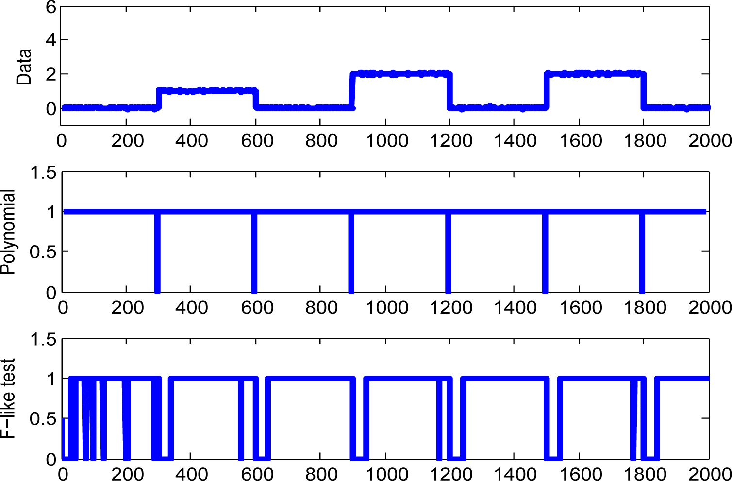
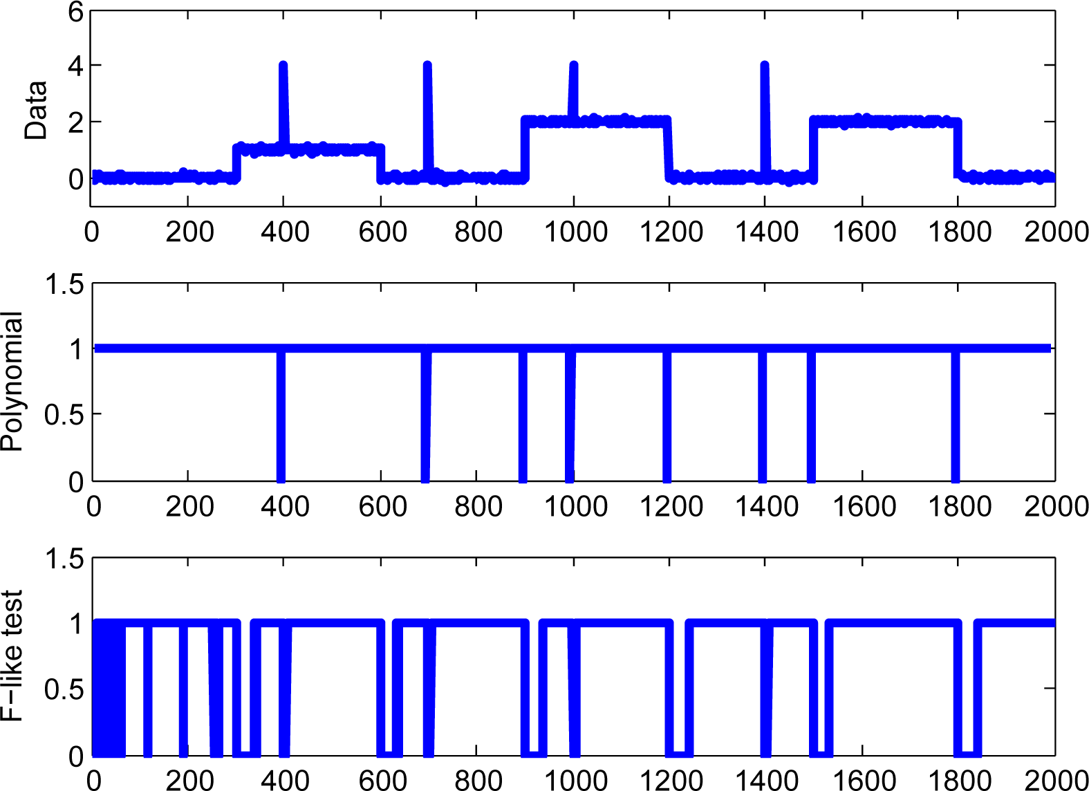
3.1. Simulated Dataset

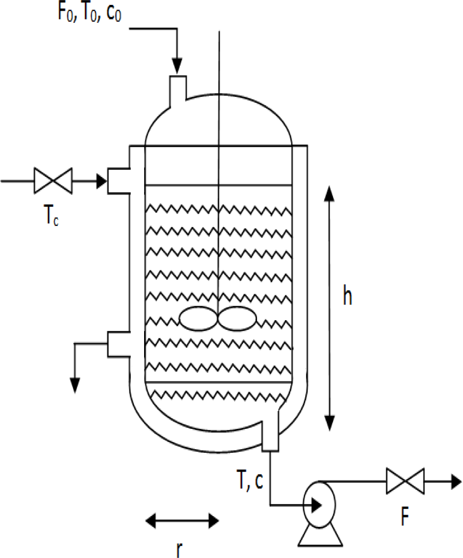
The simulated dataset case is designed for the preliminary performance evaluation of the techniques. This case allows us to have complete control of the steady-state periods, as presented in Tao et al. [22]. Simply stated, for the data simulation, a constant signal with the addition of a Gaussian noise is defined for a certain time window. To generate non-steady-state periods, steps are applied to the original signal.

Two case studies are performed using the simulated data. In the first study, 3% of the noise is added to the simulated data. In the second study, gross error is also included in the simulated data with 5% of noise, which provide additional realism to the studies. Figures 1 and 2 present in their top part the datasets for these studies. These datasets will be employed for checking the performance of the techniques and for proposing tuning modifications when necessary. The polynomial, wavelet and the F-like test techniques will be considered in this case, as they only use the measurement information from process outputs for identifying the steady-state/unstable condition. The reactor system presented next will allow the evaluation of the techniques with potential for online implementation, a category that includes our novel ARX-based approach.

3.2. CSTR System

A CSTR is used for evaluating the steady-state techniques with the online potential mentioned above. A first-order and irreversible reaction, A−>B, in the liquid phase occurs with external cooling for regulation of the reactor temperature (see the process schematic in Figure 3 and the parameters in

Table 1. Parameters of the CSTR.

Parameters	Name	Value
k0	frequency factor	7.210 × 1010 min−1
F0	inlet flow rate	0.1 m3/min
C0	concentration of A in the inlet flow	1 mol/m3
r	radius of the tank	0.219 m
Tc	coolant liquid temperature	300 K
U	heat transfer coefficient	54,936 J/(min m2 K)
h	level of the tank	0.659 m
E/R	activation energy and gas constant	8.75 × 103
T0	temperature of the inlet flow	350 K
−∆H	heat of reaction	5.7 J/mol
ρ	density	1 × 103 kg/K
Cp	specific heat capacity	239 J/(kg K)

). In this case, the level is assumed constant. The mass and energy balances that represent this system are given by the following differential equations [23,24]:

$$\frac{dC}{dt}=\frac{F_0\left(C_0-C\right)}{\pi rh}-k_{0}C\exp \left(-\frac{E}{RT}\right)$$

(21)

$$\frac{d{T}_r}{dt}=\frac{F_0\left(T_0-T\right)}{\pi r^{2}h}-\frac{-\mathrm{\Delta }H}{\rho C_p}{k}_{0}C\exp (-\frac{E}{RT}+\frac{2U}{r\rho C_p}(T_c-T_r)$$

(22)

Normally, chemical processes have controllers to manipulate the process inputs in order to achieve different steady states. As this CSTR system presents highly nonlinear behavior, a nonlinear model predictive control (MPC) approach is implemented during the transitions to drive the system from one steady state to another [25]. This MPC implementation also enables the application of the SSI methods under more realistic process conditions. In a typical hierarchical process control structure, such a controller would be placed under an RTO scheme that uses SSI to help define its models as motivated above. In this system, the following variables are considered: two controlled variables, y = [C, T_r], the concentration of A and reactor temperature, respectively; and two manipulated inputs, u = T_c, coolant liquid temperature, and u = F₀, the inlet flow rate. The optimization problem solved by the controller at each time step is given by:

$$min{\displaystyle \sum _{i=1}^p{\Vert y(k+i)-y_{sp}\Vert }_Q^2}+{\displaystyle \sum _{i=0}^{m-1}{\Vert \mathrm{\Delta }u(k+i)\Vert }_R^2}$$

(23)

subject to:

$$\begin{array}{c}{u}_{min}\le u(k+i)\le u_{max},i=0,\cdots ,m-1\\ \left|\mathrm{\Delta }u(k+i)\right|\le \mathrm{\Delta }{u}_{max},i=0,\cdots ,m-1\\ \text{Equations}\left(21\right)\text{and}\left(22\right)\end{array}$$

where p is the prediction horizon, m is the control horizon, Q and R are symmetric positive definite weighting matrices, which were tuned by trial and error, and y_sp is the output setpoint.

For the controller implementation, time derivatives of the mass and energy balances were discretized using a forward finite difference scheme and an integration step of 10 seconds. The problem was written in GAMS 24.1.3 [26] and solved with IPOPT [27]. In the two top parts of Figure 4, the closed-loop results for a case with 3% of noise added to the measurement with different setpoints during the simulation are presented. The information of the concentration was not used for the present study, because measurements of this state are not normally available in chemical processes. The SSI for estimated states was the subject of investigation in [16].

3.3. Industrial Depropanizer Column

In Figure 5, the process flowsheet schematic of the depropanizer unit operated by PETROBRAS S.A. is presented (proprietary details are omitted). Simply stated, a hydrocarbon mixture is expanded in valve V3 before entering the distillation tower T-3 that has 197 stages. The main bottom product of the tower in Stream 27 is propane, which is sent to the splitter SB3 that separates the part sold to the market from the other part to be used in the reboiler (RB3). The light products of the tower in Stream 18 are mixed with Stream 25, which comes from the distribution tank TA1. The components of this mixed Stream 19 are then compressed in C1, which increases the pressure in the stream until condensation is possible in RB3. The splitter SC1 sends part of the vapor to heat exchanger HX4 for condensation and the larger proportion to RB3. The liquids from RB3 and HX4 are expanded through valves V5 and V4, respectively, and later sent back to the tank.

The process model that describes this unit is highly nonlinear, and the pieces of equipment are highly interconnected, as observed in the above description. Furthermore, the detailed version of the model of this process is composed by ≈9,338 variables and represented by differential and algebraic equations. This process is under study for the implementation of a real-time optimization framework based on an equation-oriented simulation environment. For this reason, the identification of the steady states is essential as motivated above. Due to the high-dimensionality characteristics of the original system, we analyze here the SSI involving individual pieces of equipment, namely the reflux drum (TA1) of the column and the heat exchanger (HX4), for simplification purposes. A full-scale SSI problem would be tackled by using the product operator of the SSI results for each variable [3], i.e., if only one variable is not at steady state, the process is considered in transient condition. In this analysis, real process data are considered for the studies. Figure 6 depicts the temperature experimental data for an entire month period of the TA1 outlet Stream 24, which corresponds to an output dataset. Furthermore, Figures 7 and 8 show the level (controlled variable) and flow rate (manipulated variable) of the heat exchanger (HX4) for a month of operation, which is an input-output dataset. To address these cases, first the polynomial, wavelet and the F-like test are implemented for the reflux drum dataset. Then, the selected output-based methods, as well as the proposed ARX-based approach are evaluated for the heat exchanger input-output data.

4. Steady-State Identification Results

This section presents the analysis of the SSI results for the systems described above. Throughout this section, one and zero indicate whether the system is at steady state or not, respectively. For each category of examples (theoretical/industrial), the traditional methods (F-test, polynomial, wavelet) are implemented first, followed by the inclusion of the ARX-based approach in the subsequent test cases. For all of the techniques, the tuning parameters mentioned in Section 2 are initially considered. In case such techniques do not show satisfactory performance, the tuning parameters are changed, and their new values are reported.

4.1. Simulated Data Example

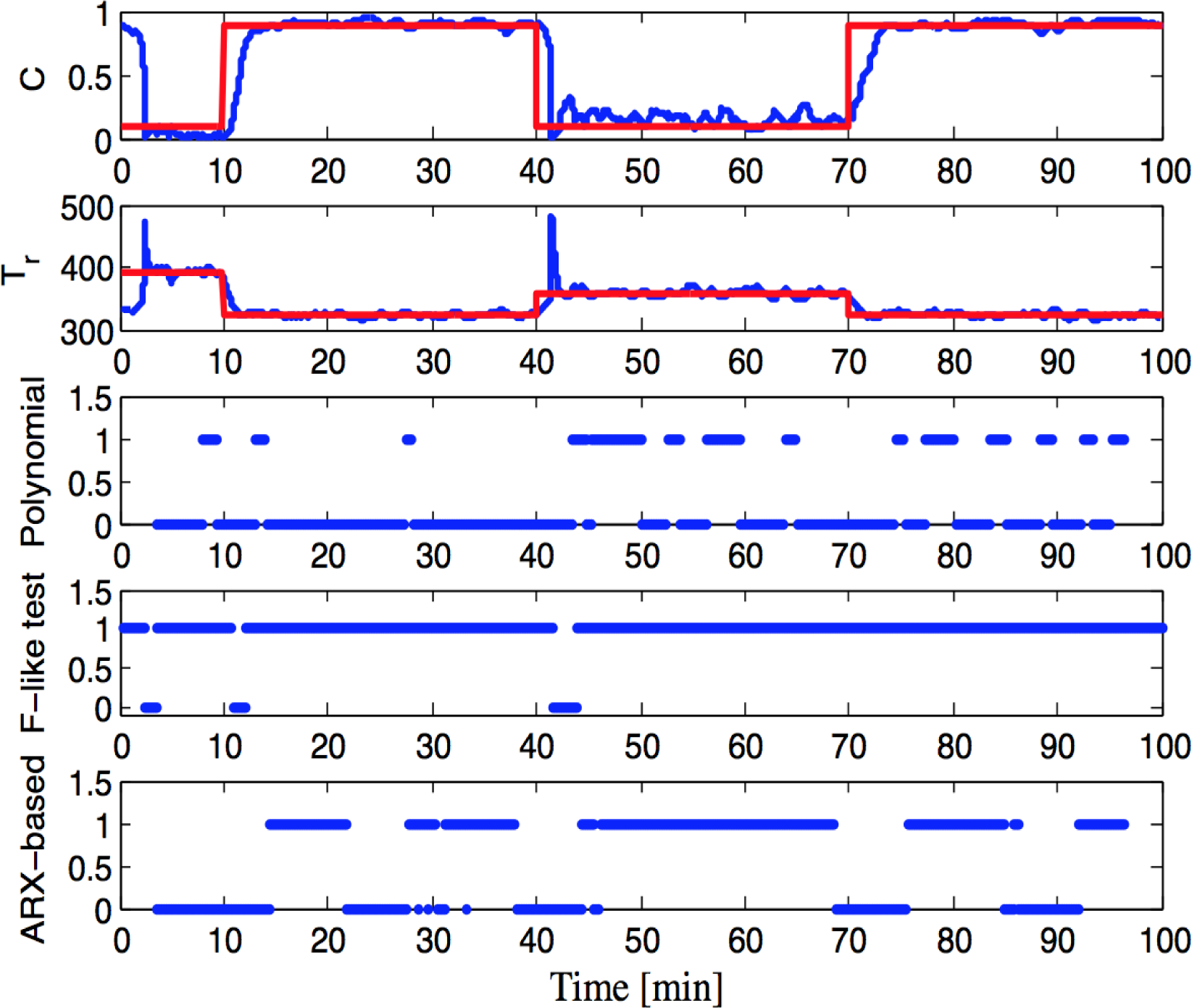
The simulated dataset is addressed with the F-like test, polynomial and wavelet techniques. This dataset provides a simple scenario for evaluation of these methods. In this case, our proposed ARX-based approach is not considered due to the absence of process inputs in this dataset. For both cases involving the simulated datasets, the initial simulations with the polynomial technique using the original index defined by Equation 10 did not produce a satisfactory performance. Due to this lack of performance, the polynomial technique index was changed to $\lambda =\frac{30\sigma }{N}$with N = 10. Furthermore, the parameters of the F-like test, λ₁ = 0.0587, λ₂ = 0.3, λ₃ = 0.02, were taken from

Table 2. Success rate of steady-state identification (SSI) methods for different frequencies for the HX4 case.

Frequency	F-Like Test	Wavelet	ARX-Based
1	37%	30%	46%
3	50%	60%	83%
5	56%	88%	92%

of [13], because these factors improved the performance of the method, and a λ = 1.2 was employed for the wavelet approach.

Figure 1 depicts in the top part, denoted as Data, the variation of the steady state for the first simulated process. This process is changing to different steady states with values of zero, one and two with 3% of noise for a total of seven steady-state periods. As the results show in the middle part of Figure 1, the polynomial technique successfully identified all of the steady states with the selected window. In the bottom part of the figure, the F-like test results present less accuracy in the identification of the steady states for the simulated data.

Figure 2 presents the performance of the two approaches (F-like test and polynomial) when four gross errors and 5% of noise are considered in the second case. As the results show in the middle part of the figure, the polynomial technique with a window size of 10 successfully identified all four gross errors and most of the steady states. However, for a system of higher complexity, the tuning of the constant parameter in the index equation would have to be carefully defined. On the other hand, the F-like test missed the identification of steady states in the beginning of the dataset, but performed well after a time of 400 units, as shown in the bottom part of Figure 2. It is worth mentioning that when these methods are connected to other frameworks that require SSI, such successful identification would be necessary at least once during the sampling period. Thus, depending on the process operating region, the results of the F-like test could also be considered satisfactory with the assumed tuning parameters.

The wavelet method is also implemented after filtering the simulated data associated with the second case. This step is necessary for the calculation of the first and the second derivatives employed to define the SSI index. Figure 9 presents the SSI results obtained with the wavelet method. Note that this method was able to identify all of the transients and gross errors as observed in the lower part of the figure, where these 10 identified unstable points are represented by discontinuities.

4.2. CSTR System

For the CSTR system, two simulations are performed (with 3% of noise) using the three SSI techniques with higher potential for online application. The wavelet method is not considered here, due to its original offline nature (see the industrial case below for a comparison between the proposed method and the wavelet). In the first simulation, the polynomial and ARX-based techniques use a window of 70. As mentioned above, the eigenvalue threshold for the ARX-based technique is 10⁻², i.e., below this value, the process is considered at steady state. To build the ARX model matrix, information is taken from the manipulated input u = T_c and the controlled output y = T_r. The other techniques only used information of the controlled output y = T_r. Finally, the F-like test considered the following tuning parameters, λ₁ = 0.2, λ₂ = λ₃ = 0.1.

Figure 4 presents the results for the above conditions, in which the red lines correspond to the process setpoints. In this case, the polynomial technique showed less accuracy in the identification of the steady-state conditions by determining that the process is transient for the majority of time. The F-like test obtained good performance during most of the SSI period. Particularly, this test only missed identifying the transients at Time 70 and at the beginning of the simulation. The ARX-based technique performed slightly better than the polynomial approach, but still had issues with the steady-state detection at several data points. In order to improve the performance of these two approaches, the size of the specified windows will be reduced in the next simulation.

For the second simulation, the tuning parameters of the analyzed techniques are modified. Specifically, the size of the window for the ARX and the polynomial approaches is reduced to 30. Furthermore, the F-like test parameters are updated to λ₁ = 0.0587, λ₂ = 0.3, λ₃ = 0.02. Figure 10 presents the results for these new conditions. Note in this figure that the polynomial technique improved its performance when compared to the previous case. However, the technique still fails to indicate the steady-state condition at some points, for example during the time interval between 15 and 25. For guaranteed performance, the polynomial technique may need further development, including further studies on its index definition. The F-like test with the new tuning is now able to identify the transients at Time 70 and at the first instants. Finally, the ARX-based technique considerably improved its performance after re-tuning, showing comparable results to the F-like test, with less Type-I errors. From the number of tuning parameters point of view, the ARX-based approach requires the size of the window and the threshold (ϵ), which has an intuitive definition, as it depends on the singularity of the model matrix. The F-like test is based on three λ’s. The above results indicate that the ARX-based technique offers an alternative with comparable performance to the F-like test, but with less tuning parameters.

4.3. Industrial Depropanizer Column

In this section, the industrial datasets of the depropanizer process (shown in Figure 5) are analyzed considering two cases for the implementation of the F-like test, the polynomial, the wavelet and ARX-based techniques. As mentioned above, we focus this study on datasets from selected pieces of equipment that describe the industrial process. However, the methodology developed in this work can also be applicable to other parts of the process.

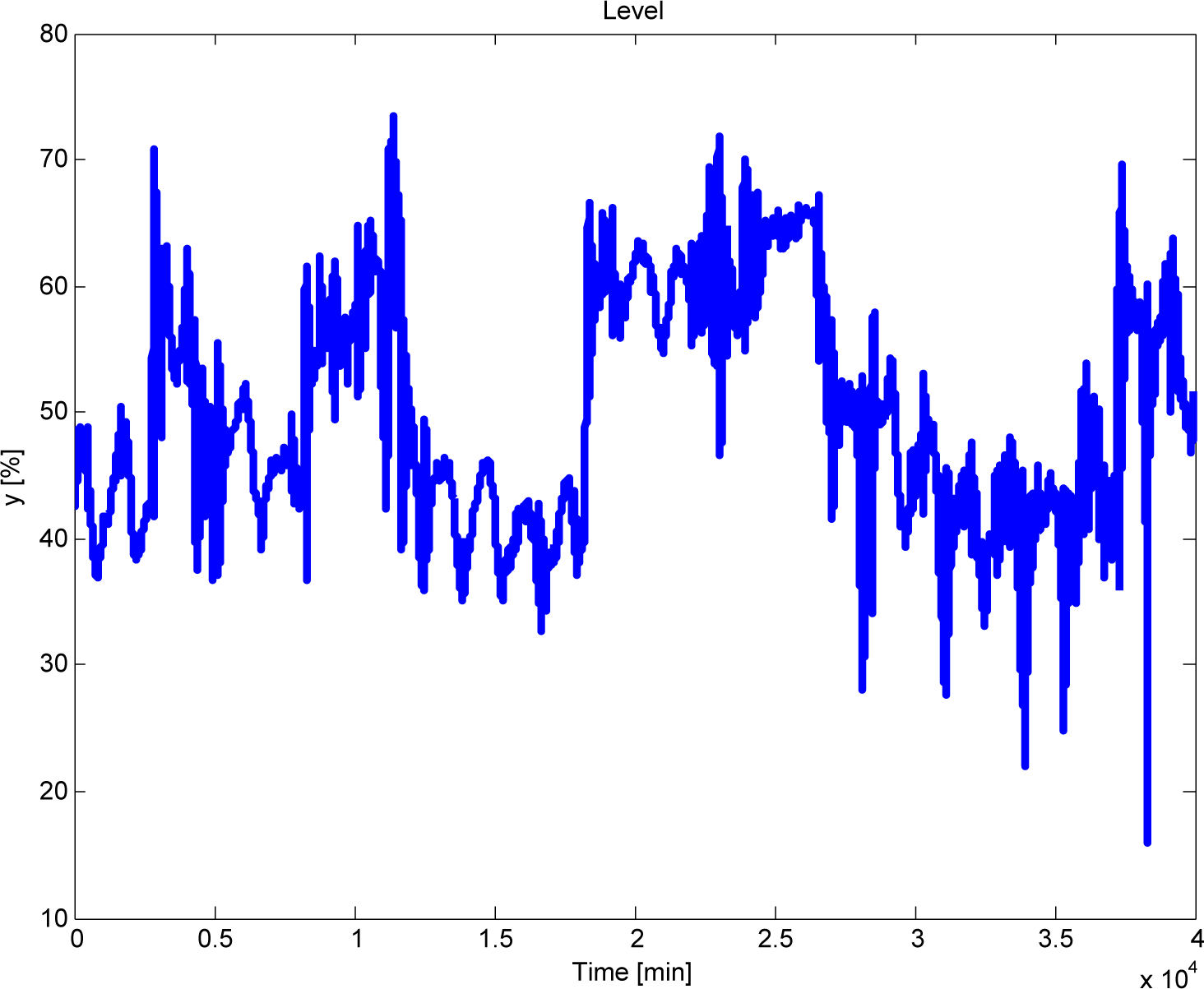
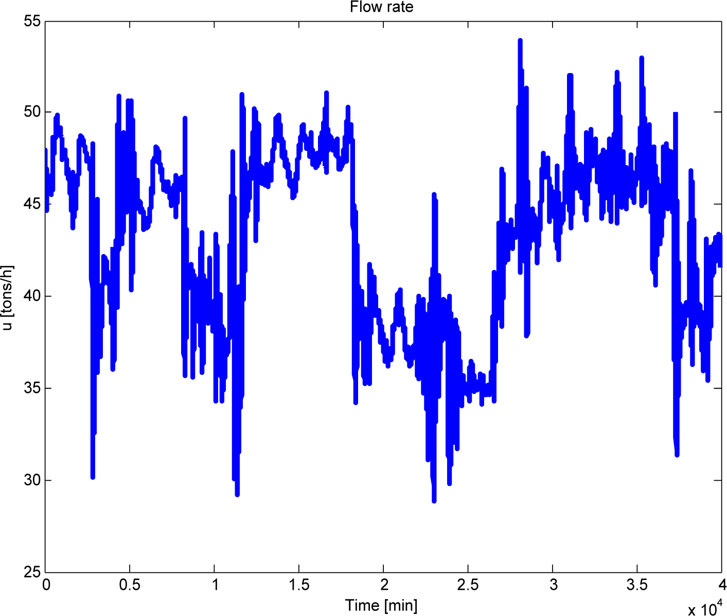
4.3.1. Analysis of the Reflux Drum (TA1)

In this subsection, the output dataset associated with the reflux drum (TA1) of the depropanizer process is analyzed to evaluate the output-based SSI methods (see the next case for an input-output study). The experimental data considered here were provided by PETROBRAS S.A. with a frequency of 1 min for each measurement. These data were taken directly from the data acquisition equipment, i.e., without pre-filtering. For this study, the temperature at the exit of the tank in Stream 24 is used for the comparison of the aforementioned techniques. In particular, portions of the original data depicted in Figure 6 are considered for SSI. The first portion is shown in the top part of Figure 11 and corresponds to two steady-state periods (from test Days 18 at 09:22:00 a.m to 19 at 08:42:00 a.m.) with a transient in between. These periods were defined by visual inspection of the dataset. Figures 11 and 12 present the results of the techniques employing the following tuning: a window of 30 for the polynomial approach, λ₁ = 0.0587, λ₂ = 0.3, λ₃ = 0.02 for the F-like test and a λ = 1.2 for the wavelet method.

Figure 11 shows a lack of performance of the F-like test and the polynomial techniques for the clear steady-state condition at the beginning and the end of the experimental data. Several tuning parameters (window sizes and λ’s) were tested for these methods in order to improve the results without success. On the other hand, Figure 12 shows the correct identification of the transient data by the wavelet method between 600 and 1,000 min. Due to the smooth characteristics of the original data, the filtering step in the wavelet method implementation was not necessary. In an attempt to improve the performance of the variance-based methods, namely the F-like test and the polynomial, a scenario in which an artificial additional Gaussian noise of 5% was added to the experimental data is considered. Figures 13 and 14 present the steady-state detection results for this scenario associated with the F-like test, the polynomial and wavelet approaches with the same tuning parameters previously mentioned. Differently from the previous results, Figure 13 shows improvement in the SSI by both the polynomial and F-like techniques. The polynomial technique presents a complete identification of the transient period in the middle of the data with some scattered misses in the SSI during the beginning and the end of the set. The F-like test shows better results, in which the identification of the steady states at the tails of the dataset is satisfactory with only some spare failings at some points. Figure 14 presents the wavelet results when the noise is added to the experimental data. Here, the wavelet method is no longer accurate, as it was previously. Therefore, these results indicate that the noise level in the dataset plays a critical role in the performance of the methods. The variance-based methods needed the presence of the noise for improved performance. On the other hand, the wavelet approach demands a smoother experimental dataset (with a high level of filtering) for accuracy. This is an important conclusion for industrial processes in which noisy datasets are generally observed. Thus, depending on the implemented method of choice, careful attention must be paid in terms of data processing prior to the steady-state identification.

The second portion of the temperature data in Figure 6 corresponding to a different time period is now considered (between test Day 06 at 3:34:00 p.m. until day 09 at 07:53:00 a.m.). These data depicted in the top part of Figure 15 present a different challenge for the methods, as stable periods occur from about 0–600 min and 1,200–1,700 min, with a transient behavior in the rest of the data. Figures 15 and 16 show the results of SSI of this dataset using the output-based methods. Note in Figure 15 that the polynomial technique identified some steady-state points before 600 min, but it missed detecting whole periods, for example the transient one from 2,000–2,500 min. The F-like test obtained a much better result using the last tuning parameters mentioned. As it is possible to observe in the lower part of Figure 15, the F-like test correctly pointed out most of the steady-state period before 600 min. After that point, it obtained satisfactory performance given the dataset variability, except for the part between 1,400 and 1,600 min. The results of the wavelet method with a new λ = 0.1 (used for enhanced performance) are presented in Figure 16 in which the stable periods were efficiently identified before 600 min and from 1,200–1,700 min. This method once again shows improved performance when compared to the other output-based counterparts, with only minor errors for some scattered points before 1,200 min and in the final period of transient behavior from 2,000–2,500 min.

4.3.2. Loop Data from the Heat Exchanger (HX4)

In this case, we analyze the proposed ARX-based approach in an industrial setting by using a complete input-output dataset for the steady-state identification. Although this approach requires additional process information, its implementation still maintains the relative degree of simplicity. A loop of the heat exchanger (HX4) presented above is considered for studying the behavior of the methods assuming different measurement frequencies (1, 3, 5 min). This frequency analysis will permit the identification of the sampling effect in the performance of the methods. The experimental data now correspond to the level (output, y) and the inlet flow rate (input, u) taken from the original data depicted in Figures 7 and 8. The purely output-based methods selected for this example are the F-like test and the wavelet techniques based on their better performance than the polynomial approach in the above cases. Figure 17 presents the results of the methods for a measurement frequency of 1 min and with the following tuning: a window of 5 for the ARX-based method, λ₁ = 0.0587, λ₂ = 0.3, λ₃ = 0.02 for the F-like test and a λ = 0.06 for the wavelet approach. In this figure, the top two parts depict the data associated with the output and input variables. These variables show a transient behavior in the first 410 min, followed by a steady-state period. The results of the F-like test in this figure show that this approach is able to correctly identify the steady-state part after 400 time units. However, the initial period was not identified properly. The wavelet method performs in a similar manner by missing most of the transient periods between 0 and 400 min, but detecting the steady-state period afterwards. The ARX-based approach has a slightly better performance. It identified correctly the entire steady-state period after 400 time units, and the transient parts between 60–160 and 300–340 min.

In the next case, we analyze the performance of the methods assuming the same dataset, but with a measurement frequency of 3 min. The results for this new frequency are presented in Figure 18. Note that the F-like test improves the identification of the unstable condition from 0–120 min when compared to the case in Figure 17. Likewise, the wavelet approach enhanced considerably its performance by pointing out transient periods that were not identified with a frequency of 1 min (see Figure 18). For the ARX-based method, the unstable period was detected with even a greater precision with this new frequency, as observed in Figure 18, in which it mostly missed the transient from 250–300 min. Similarly to the previous results, the proposed ARX-based approach shows an improved performance when compared to other methods considered.

As a final case study, a measurement frequency of 5 min is assumed for the data collection step, and the obtained data are presented in the top two portions of Figure 19. This same figure also shows the final results for all methods assuming the same tuning as in the previous case. In these results, the F-like test shows small progress when compared to the previous case, but still has issues in the identification of the unstable period from 180–310 min. On the other hand, the wavelet and ARX-based methods obtained SSI results of higher accuracy. Specifically, for the transient period, the wavelet method now mostly missed detecting the points between 250 and 290 min, while the ARX-based approach has no error in this period when considering a method threshold of = 10⁻³. The steady-state period was once again correctly identified by both the ARX-based and the wavelet methods, in which the ARX-based one only missed some stable points around 410–430 min. Thus, both methods demonstrated a satisfactory level of accuracy for this application. Table 2 summarizes the SSI results for different frequencies in terms of their success rate in identifying steady-state/transient points. Therefore, this case study shows that the performances of the methods improve when reducing the measurement sampling. This conclusion suggests that, for really fast sampling, the SSI analysis is giving a higher weight to the faster dynamics (including local noises and oscillations), rather than the overall dynamic characteristics of the system that are relevant to the steady-state detection. It is also important to note that depending on the noisy characteristics of the dataset, the wavelet method may require a data pre-filtering step (for the correct calculation of the first and second derivatives), which would preclude its online implementation. That is not the case of our proposed ARX-based approach that uses a model that is computationally tractable for online application.

5. Conclusions

This paper analyzed four SSI techniques: the available F-like test, the polynomial-based approach and the wavelet method, as well as the proposed novel ARX-based method. For the analysis, three case studies were selected. In the first case, the methods that depend only on output measurements (polynomial, wavelet and F-like test) were initially tuned and compared using a simulated dataset. The results of this case showed a better performance of the polynomial and the wavelet approaches when compared to the F-like test, after careful tuning of their parameters. The second case, a CSTR model coupled with a nonlinear model predictive controller, provided a setup for the comparison of three techniques with higher potential for online implementation (F-like test, polynomial approach and ARX-based method) under more challenging operating conditions. The results of this implementation presented equivalent performance for the F-like test and the ARX-based techniques (that was better than the polynomial method) after changing the tuning parameters associated with their SSI indexes. In the third case, industrial process data from a refinery operated by PETROBRAS S.A. were used considering two different pieces of equipment associated with a depropanizer column: the reflux drum and the heat exchanger. Two temperature (output) datasets for the reflux drum case were analyzed using the polynomial, the F-like test and the wavelet approaches. The results showed that the F-like and the polynomial technique have improved performance for industrial datasets of noisy characteristics, as opposed to the wavelet method, which requires a data pre-filtering step for relatively smoother data. In a final example with the heat exchanger input-output data, selected output-based techniques, namely the F-like test and the wavelet method, as well as the ARX-based approach were considered. The results for this implementation indicated that the selection of the measurement sampling rate is critical for SSI of industrial datasets. This rate determines the importance of local vs. overall process dynamics in the SSI. In particular, the ARX-based method and the wavelet approach overcame the performance of the F-like test and presented satisfactory SSI results for this case for a measurement sampling frequency of 5 min. In this study, the robustness of the SSI techniques was not considered. For that purpose, a Monte Carlo analysis would have to performed, which would enable the construction of pdf graphs associated with the SSI results.

After these studies, we have the following overall recommendations and conclusions for researchers and industrial practitioners: (i) the F-like test and the polynomial approaches have the advantages of their relatively simple implementation requiring only output datasets; however, a really careful tuning analysis must be carried out for the practical application of these methods; (ii) the wavelet method, which is also output-based, has a higher level of sophistication when compared to the F-like test and the polynomial methods, but requires a data pre-filtering step for accurate performance; and (iii) our proposed ARX-based approach provides a new alternative that has the greatest SSI precision in general when compared to the other methods. Although this approach needs input-output datasets for its implementation, it has the advantage of incorporating the system dynamics through a computationally tractable ARX model for online application. As future work, the SSI results of the depropanizer column will be incorporated into an RTO software solution that is currently under development for PETROBRAS S.A.

References

1. Biegler, L.T.; Lang, Y.; Lin, W. Multi-scale optimization for process systems engineering. Comput. Chem. Eng. 2014, 60, 17–30. [Google Scholar]
2. Korbel, M.; Bellec, S.; Jiang, T.; Stuart, P. Steady state identification for on-line data reconciliation based on wavelet transform and filtering. Comput. Chem. Eng. 2014, 63, 206–218. [Google Scholar]
3. Rhinehart, R.R. Automated steady and transient state identification in noise processes. Proceedings of the American Control Conference, Washington, DC, USA, 17–19 June 2013; pp. 4477–4493.
4. Cao, S.; Rhinehart, R.R. An efficient method for on-line identification of steady state. J. Proc. Cont. 1995, 5, 363–374. [Google Scholar]
5. Cao, S.; Rhinehart, R.R. Critical values for a steady-state identifier. J. Proc. Cont. 1997, 7, 149–152. [Google Scholar]
6. Shrowti, N.; Vilankar, K.; Rhinehart, R.R. Type-II critical values for a steady-state identifier. J. Proc. Cont. 2010, 20, 885–890. [Google Scholar]
7. Rhinehart, R.R. Automated steady-state identification: Experimental demonstrations. J. Proc. Anal. Chem. 2002, 7, 1–4. [Google Scholar]
8. Rhinehart, R.R. A statistically based filter. ISA Trans. 2002, 41, 167–175. [Google Scholar]
9. Vennavelli, A.N.; Resetarits, M.R. Demonstration of the SS and TS Identifier at the Fractionation Research, Inc. (FRI) Distillation Unit, Proceedings of the American Control Conference, Washington, DC, USA, 17–19 June 2013; pp. 4494–4497.
10. Brown, P.R.; Rhinehart, R.R. Demonstration of a method for automated steady-state identification in multivariable system. Hydrocarb. Process 2000, 79, 79–83. [Google Scholar]
11. Iyer, M.S.; Rhinehart, R.R. A novel method to stop neural network training. Proceedings of the American Control Conference, Chicago, IL, USA, 28–30 June 2000; pp. 929–933.
12. Rhinehart, R.R.; Su, M.; Manimegalai-Sridhar, U. Leapfrogging and synoptic Leapfrogging: A new optimization approach. Comput. Chem. Eng. 2012, 40, 67–81. [Google Scholar]
13. Bhat, A.S.; Saraf, D.N. Steady-state identification, gross error detection, and data reconciliation for industrial process units. Ind. Eng. Chem 2004, 43, 4323–4336. [Google Scholar]
14. Kim, M.; Yoon, S.H.; Domanski, P.A.; Payne, W.V. Design of a steady-state detector for fault detection and diagnosis of a residential air conditioner. Int. J. Refriger 2008, 31, 790–799. [Google Scholar]
15. Kelly, J.D.; Hedengren, J.D. A steady-state detection (SSD) algorithm to detect non-stationary drifts in processes. J. Proc. Cont. 2013, 23, 326–331. [Google Scholar]
16. Flehmig, F.; Marquardt, W. Inference of multi-variable trends in unmeasured process quantities. J. Proc. Cont. 2008, 18, 491–503. [Google Scholar]
17. Jiang, T.; Chen, B.; He, X. Industrial application of Wavelet Transform to the on-line prediction of side draw qualities of crude unit. Comput. Chem. Eng 2000, 24, 507–512. [Google Scholar]
18. Jiang, T.; Chen, B.; He, X.; Stuart, P. Application of steady-state detection method based on wavelet transform. Comput. Chem. Eng. 2002, 27, 569–578. [Google Scholar]
19. Korbel, M.; Bellec, S.; Jiang, T.; Stuart, P. Steady state identification for on-line data reconciliation based on wavelet transform and filtering. Comput. Chem. Eng. 2014, 63, 206–218. [Google Scholar]
20. Yao, Y.; Zhao, C.; Gao, F. Batch-to-batch steady state identification based on variable correlation and mahalanobis distance. Ind. Eng. Chem. 2009, 48, 11060–11070. [Google Scholar]
21. Le Roux, G.A.C.; Santoro, B.F.; Sotelo, F.F.; Teissier, M.; Joulia, X. Improving steady-state identification, Proceedings of the 18th European Symposium on Computer Aided Process Engineering, ESCAPE 18, Lyon, France, 1–4 June 2008; pp. 459–464.
22. Tao, L.; Li, C.; Kong, X.; Qian, F. Steady-state identification with gross errors for industrial process units, Proceedings of the 10th World Congress on Intelligent Control and Automation, Beijing, China, 6–8 July 2012; pp. 4151–4154.
23. Pannocchia, G.; Rawlings, J.B. Disturbance models for offset-free model-predictive control. AIChE J 2003, 49, 426–437. [Google Scholar]
24. Henson, M.A.; Seborg, D.E. Nonlinear Process Control; Prentice Hall PTR: Upper Saddle River, NJ, USA, 1997. [Google Scholar]
25. Findeisen, R.; Allgöwer, F. An introduction to nonlinear model predictive control. Proceedings of the 21st Benelux Meeting on Systems and Control, Veldhoven, The Netherlands, 19–21 March 2002; 11, pp. 119–141.
26. Brooke, A.; Kendrick, D.; Meeraus, A.; Raman, R. User’s Guide; GAMS Development Corporation: Washington DC, USA, 1998. Available online: http://www.gams.com accessed on 4 January 2015.
27. Wachter, A.; Biegler, L.T. On the implementation of primal-dual interior point filter line search algorithm for large-scale nonlinear programming. Math. Program 2006, 106, 25–57. [Google Scholar]
Figure 1. Case 1. Simulated data results with 3% of noise, in which a window of 10 was used for the polynomial technique.
Processes 03 00257f1
Figure 2. Case 2. Simulated data results with 5% of noise with gross error, in which a window of 10 was used for the polynomial technique.
Processes 03 00257f2
Figure 3. Schematic representation of the continuous stirred-tank reactor (CSTR).
Processes 03 00257f3
Figure 4. CSTR data results with 3% of noise, in which a window of 70 was used for the polynomial and the ARX-based techniques.
Processes 03 00257f4
Figure 5. Depropanizer process flowsheet.
Processes 03 00257f5
Figure 6. Temperature experimental data of Stream 24 for a month period.
Processes 03 00257f6
Figure 7. Level experimental data of heat exchanger HX4 for a month period.
Processes 03 00257f7
Figure 8. Flow rate experimental data of HX4 for a month period.
Processes 03 00257f8
Figure 9. Case 2. Simulated data results for filtered data using the wavelet technique.
Processes 03 00257f9
Figure 10. CSTR data results with 3% of noise, in which a window of 30 was used for the polynomial and the ARX-based techniques.
Processes 03 00257f10
Figure 11. Depropanizer reflux drum case temperature experimental data and SSI results for the F-like test and the polynomial methods.
Processes 03 00257f11
Figure 12. Depropanizer reflux drum case temperature experimental data and SSI results for the wavelet method.
Processes 03 00257f12
Figure 13. Depropanizer reflux drum case temperature experimental data, in which 5% of Gaussian noise is added to the data, and the SSI results for the F-like test and the polynomial methods.
Processes 03 00257f13
Figure 14. Depropanizer reflux drum case temperature experimental data, in which 5% of Gaussian noise is added to the data, and the SSI results for the wavelet method.
Processes 03 00257f14
Figure 15. Depropanizer reflux drum case temperature experimental data and SSI results for the F-like test and the polynomial methods.
Processes 03 00257f15
Figure 16. Depropanizer reflux drum case temperature experimental data and SSI results for the wavelet method.
Processes 03 00257f16
Figure 17. HX4 input-output case with a measurement frequency of 1 min.
Processes 03 00257f17
Figure 18. HX4 input-output case with a measurement frequency of 3 min.
Processes 03 00257f18
Figure 19. HX4 input-output case with a measurement frequency of 5 min.
Processes 03 00257f19