1. Introduction
Polymers are continuously substituting traditional materials (e.g., glass, woods and metals) along with low cost and good processability. Polyethylene terephthalate (PET) is the most common thermoplastic polymer resin, which is the primary raw material for synthetic fibers, dielectric films and beverage bottles. PET has dominated the synthetic fibers industry over the years accounting for nearly half of the global consumption [
1]. Moreover, the global demand for PET is predicted to grow in the next few years. Therefore, producing PET with the required properties is of major industrial importance.
It is well known that the end-use properties of PET, such as drawing behavior, melting point, tensile strength and thermal stability, strongly depend on its molecular weight and byproduct concentrations [
2,
3,
4,
5]. There are several side reactions taking place along with the main polycondensation reaction. The amount of side products (
i.e., diethylene glycol (DEG), acetaldehyde, water, carboxyl end groups, vinyl end groups) determines the quality and properties of the final PET product. For example, every one percent of DEG in the polyester chain will cause a lower melting point by 5 °C [
6]. Additionally, even a small amount of DEG leads to reduced heat resistance, decreased crystallinity and UV light stability. Vinyl end groups may also be polymerized with other polyester chains to form polyvinyl ester, of which the pyrolysis products have been shown to be responsible for the coloration of PET [
7]. A high initial concentration of carboxyl groups could induce a decrease in the degree of polymerization (DP) due to hydrolytic degradation [
8]. In order to ensure product quality, the amount of byproducts needs to be well controlled within certain limits.
However, the monitoring and control of polymerization reactors is not an easy task, owing to a lack of fast on-line measurements and the significant nonlinearity of the processes. Very often, critical quantities related to safety, product quality and/or economic performance of a polymerization process cannot be measured on line. Thus, state estimation plays an important role in providing frequent and reliable information of the process, which can be integrated into model-based control, as well. Since the early 1980s, there have been significant efforts in the design and application of state estimators to polymerization reactions, especially in free radical polymerization. The extended Kalman filter (EKF), as an industrially-popular estimator, has been widely used and achieved fairly good performance in many cases [
9,
10,
11,
12,
13,
14,
15,
16]. In this approach, the design is based on an approximate local linearization of the system along a reference trajectory. Even though EKF has found industrial applications, there have been studies that established its serious difficulties in the presence of strong process nonlinearities [
17,
18]. An alternative approach for estimation in polymerization processes is state observer design [
19,
20,
21,
22,
23,
24,
25,
26]. It utilizes the dynamic process model, which captures the evolution of physical and chemical phenomena, and then generates a soft sensor that is able to reconstruct the missing state variables with additional appropriate feedback terms from all of the on-line measurements. For example, Van Dootingh
et al. [
19] developed a nonlinear high-gain observer with adjustable speed of convergence in a styrene polymerization reactor. Compared to EKF, this observer does not only have a theoretical proof of convergence, but also greatly reduces computation time. Tatiraju and Soroush [
21,
22] implemented a nonlinear reduced-order observer to a homopolymerization reactor. Along with an open-loop observer for the unobservable states, accurate estimates for all states were achieved. Astorga
et al. [
25] used a continuous-discrete observer to estimate monomer composition in an emulsion copolymerization reactor. The proposed observer was validated by comparing the outputs of the observer with off-line gas chromatography results.
Although a significant amount of work has been done in the monitoring and control of free radical polymerization reactors, very few state estimation studies are available for polycondensation reactors. Choi and Khan [
27] applied the EKF algorithm to estimate nine state variables in the transesterification stage of PET synthesis. When supplemented by five additional off-line measurements, the overall performance of the state estimator was greatly improved. Appelhaus
et al. [
28] designed an extended observer to estimate concentrations of ethylene glycol (EG) and hydroxyl end groups along with a mass transfer parameter in a batch reactor. In their study, only the reversible polycondensation reaction was considered.
A comprehensive understanding of PET synthesis is essential for effective quality control and optimization of the process. Generally, there are three stages (
i.e., transesterification/esterification, pre-polymerization and polycondensation) involved in PET production. For injection or blow molding applications, solid state polymerization needs to be carried out afterwards to obtain a product with DP over 150. In each reactor, side reactions take place simultaneously and directly affect product quality. On-line measurements for byproduct concentrations are usually not available or at relatively low sampling rates [
29]. Therefore, based on the fact that available on-line measurements are not always of the same nature, it is necessary to develop estimation/monitoring algorithms that can use all of these different kinds of on-line measurements in a synergistic way to provide valuable information of the process.
In this study, the nonlinear observer design method of exact linearization with eigenvalue assignment [
30,
31] is applied to a series of three continuous polycondensation reactors. A modified reaction-mass transfer model [
32] is used in our work. The objective is to estimate unmeasured concentrations, as well as the degree of polymerization in the PET finishing stage from continuous hydroxyl measurement and sampled acidimetric titration, where different sampling rates and time delays are considered. The basis of the observer design methodology is a continuous-time nonlinear observer design. Subsequently, an inter-sample output predictor [
33] is used to account for the slow-sampled measurements and to provide continuous estimates during the time period in between two consecutive measurements. At the same time, an estimate of the current output from the delayed measurement is obtained in the same spirit as the Smith predictor, by initializing the process model with the most recent delayed output and integrating it up to the present time. In the presence of sensor noise, a pre-filtering technique is used to cut out the noise to avoid the breakdown of the observer. The performance of the observer with inter-sample prediction and dead time compensation is evaluated by numerical simulation.
This paper is organized as follows: In
Section 2, a brief review of the reduced-order observer and sampled-data observer design methods are presented. In particular, a block triangular observer form is derived from the serial subsystem structure (e.g., multiple continuous stirred-tank reactors (CSTRs) connected in series). In
Section 3, the finishing stage of PET polycondensation, as well as its mathematical model is described. In
Section 4, the performance of the state observer is evaluated in two different cases: (i) only continuous measurement is available; (ii) both continuous and slow-sampled measurements are available. Furthermore, sensor noise is considered, and the results show that there is a tradeoff between the convergence rate and noise sensitivity. Finally, in
Section 5, conclusions are drawn from the results of the previous sections.
2. Nonlinear Observer Design Method
This section briefly outlines the main results on nonlinear observer design [
30,
31], block triangular observer design and sampled-data observer design [
33]. All of the observer synthesis and simulations in later sections are realized on the basis of reduced-order observer. Therefore, a brief necessary review is presented below.
2.1. Reduced-Order Observer
In chemical processes, on-line measurements typically involve a part of the state vector. In contrast to the full-order observer, which estimates the entire state vector, the reduced-order observer estimates only the unmeasured states. In this sense, the reduced-order observer is free of redundancies and is computationally more efficient than the full-order observer.
Consider a multi-output autonomous system whose outputs are a part of the state vector:
where
is the state vector that needs to be estimated,
is the remaining state vector that is directly measured and
is the measurement vector;
and
are real analytic functions with
,
. In the exact linearization method, the objective is to build an observer so that the resulting error dynamics is linear in curvilinear coordinates and with the pre-specified rate of decay of the error. A locally-analytic mapping
from
is sought that maps the system (1) to:
where
A is a
matrix and
B is a
matrix. The reduced-order observer in the original coordinates can be expressed as:
This leads to the following selection of the state-dependent observer gain [
31]:
where
is a solution of the following system of PDEs:
Under the above choice of observer gain, the error dynamics in transformed coordinates becomes linear and is governed by the arbitrarily-selected
A matrix:
Thus, the matrix A is a design parameter that directly adjusts the speed of convergence of the error.
Remark 1. In order to implement the above nonlinear observer design methodology, an approximate solution needs to be calculated for the system of PDEs of Equation (5). As discussed in [30,31], it is possible to approximate by using a truncated multivariable Taylor series around the origin. This requires each state expressed in deviation variable form. After expanding ,
and T in Taylor series up to a finite truncation order, the approximate solution can be obtained by equating the coefficient of each side of the PDEs. This calculation can be executed by using symbolic computation software (e.g., Maple) [31,34]. 2.2. Reduced-Order Observer in Lower Block Triangular Form
The serial CSTR reactor configuration is used in many types of chemical processes [
35,
36], leading to higher product yield and higher concentration. The serial CSTR reactor configuration usually possesses a special structure in lower block triangular (LBT) form. Additionally, this special structure can be utilized properly in state observer design to reduce the complexity of the state dependence of observer gains. Consider a system in LBT form containing three subsystems:
where I, II, III denote each subsystem, respectively. The objective of observer design is to reconstruct the missing state variables
,
and
.
Figure 1 depicts a general structure of the system in LBT form, with three subsystems.
It is intuitive to design sequential observers by taking advantage of the particular LBT structure. For example, the observer for Subsystem I is based on its unmeasured state dynamics and its own measurements and is independent of the subsequent subsystems and their measurements. The observer for Subsystem II does not only use its own dynamics and measurements, but also depends on the measurements and state estimates from Subsystem I. Moreover, its state-dependent gain depends on the gain in the first observer, as well. Thus, each observer needs to utilize the information from all of the former stages, as well as its own dynamics and measurements. In this way, it significantly reduces the computational effort of calculating the state-dependent gain symbolically.
Figure 1.
General structure of a system in lower block triangular (LBT) form with three subsystems.
Figure 1.
General structure of a system in lower block triangular (LBT) form with three subsystems.
After coordinate transformation, the observer in
z-coordinates has linear dynamics:
where both
A and
B matrix have a special LBT structure. Eigenvalues of the diagonal submatrices can be assigned arbitrarily. Since each subsystem’s observer needs the estimates from the previous subsystems, it would make intuitive sense to tune the observer for Subsystem I faster than the one for Subsystem II,
etc. Accordingly, the nonlinear reduced-order observer in original coordinates is of the form:
where the LBT state-dependent gain matrix
can be designed according to:
where
is a solution of the following system of PDEs:
Under the above observer construction, the estimation error follows linear dynamics in z-coordinates, which is governed by the A matrix. It is selected to be Hurwitz to guarantee asymptotic stability.
2.3. Sampled-Data Observer
When sampling is performed at a slow rate, inter-sample behavior becomes important and needs to be accurately estimated by the observer. For this purpose, the process model could be used to predict the evolution of output during the time period in between two consecutive measurements. The predictor is able to continuously apply a correction on the most recent sampled measurement during the sampling interval.
The inter-sample output predictor can be combined with the reduced-order observer. The original system can be appropriately expressed in partitioned form as:
where
is the state vector, which can be continuously measured,
is the sampled state variable, and
and
are the corresponding outputs. Here, the output vector is split into two parts: (
) continuous measurements and one sampled measurement.
It is possible to estimate the rate of change of the output
by utilizing the dynamic model of slow-sampled state variable. This leads to the following inter-sample output predictor:
with
ψ representing the output prediction, and
,
denote two consecutive sampling instants. The predictor is initialized at the most recent measurement
and runs until the new measurement is obtained. When the continuous-time observer of Equation (3) is driven by the output predictor of Equation (13), this generates a sampled-data observer.
Figure 2 depicts the construction of a continuous-time reduced-order observer with an inter-sample output predictor.
In earlier work [
33], it was shown that, as long as the sampling period does not exceed a certain limit, the stability of the error dynamics and robustness with respect to measurement error for the continuous-time observer of Equation (3) implies the stability of the error dynamics and robustness with respect to measurement error for the sampled-data observer. In other words, the sampled-data implementation inherits the key properties of the continuous-time design, and in fact, these properties hold at all times, not just at the sampling instants.
Figure 2.
Structure of the reduced-order sampled-data observer.
Figure 2.
Structure of the reduced-order sampled-data observer.
3. A Series of Three Polycondensation Reactors
Modeling the finishing stage of PET synthesis is quite challenging due to the complexity of reaction kinetics, coupled with mass transfer effects. For the finishing stage, plug flow reactors (PFR) are commonly used because of their uniform residence time distribution, leading to a relatively narrow molecular weight distribution. In some continuous processes, a series of CSTRs are used [
37]. The dynamics of plug flow polycondensation reactors can also be accurately modeled as multiple CSTRs in series [
38].
For simplicity, a model of three CSTR in series, which is derived from Rafler’s reaction-mass transfer model [
32], will be used throughout this study.
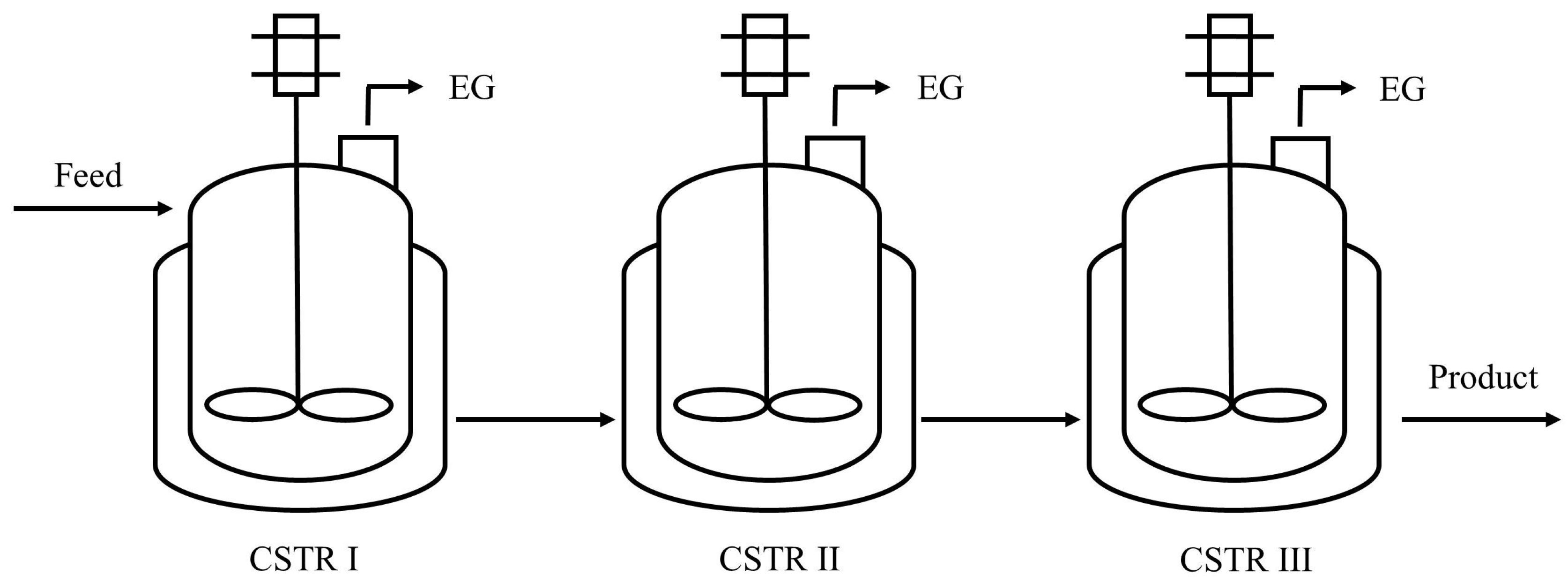
Figure 3 shows a three-CSTR in series configuration. In each reactor, the main polycondensation reaction and the thermal decomposition of ester groups are considered. Since the main reaction is reversible, EG as a byproduct has to be vaporized continuously by applying a vacuum to increase the yield of the product. The viscosity of the reaction mass also increases rapidly, which makes mass transfer a limiting factor. The dynamic process model has the following form:
All three reactors are operated at constant temperature and pressure. There are four states in each reactor: the concentration of EG (, and ), hydroxyl end groups (, and ), carboxyl end groups (, and ) and ester groups (, and ). The concentration of EG on the melt surface is denoted by the superscript *.
Figure 3.
Schematic of three CSTRs in series in the polycondensation stage.
Figure 3.
Schematic of three CSTRs in series in the polycondensation stage.
A two-film model is applied to describe mass transfer of volatiles in the finishing stage of melt polycondensation under high conversion. It is postulated that there is a concentration gradient of the volatile species throughout a liquid film near the gas-liquid interface. This is based on the existence of mass transfer resistance at the interface due to the high viscosity of the reaction mixture. Kim [
39] verified the two-phase mass transfer model from experimental data in a polycondensation system and showed that the mass transfer resistance model provided accurate prediction of molecular weight and product composition over the entire stages. The interfacial equilibrium concentration of EG is calculated by using the Flory-Huggins equation (see [
39] for equations, [
40,
41] for physical property parameters). The system parameters used in the simulations are given in
Table 1.
Table 1.
System parameters a,b.
Table 1.
System parameters a,b.
| Parameter | Description | Value |
|---|
| T | reactor temperature | 553.15 K |
| P | reactor pressure | 130 Pa |
| R | gas constant | 1.987 cal/(mol·K) |
| residence time of each CSTR | 60 min |
| rate constant of polycondensation reaction | 1.36 × 10⁶ exp(−18,500/(RT)) L/(mol·min) |
| rate constant of thermal decomposition | 7.20 × 10⁹ exp(−37800/(RT)) min-1 |
| mass transfer parameter in CSTR I | 2.70 min-1 |
| mass transfer parameter in CSTR II | 2.03 min-1 |
| mass transfer parameter in CSTR III | 1.35 min-1 |
In the reactor simulation, the following assumptions are made: (i) only EG exists in the vapor phase; (ii) mass transfer resistance on the gas side is negligible; (iii) the concentration of vinyl end groups in the feed is equal to the concentration of carboxyl end groups; (iv) the mass transfer parameter does not change over time in each reactor. The operating conditions of the reactors are given in
Table 2, where [OH], [COOH] are for hydroxyl and carboxyl end groups and [Z] is the concentration of ester groups.
Table 2.
Operating conditions and steady states a,b.
Table 2.
Operating conditions and steady states a,b.
| Concentration | CSTR# | [EG] | [OH] | [COOH] | [Z] |
|---|
| Feed | CSTR I | 6.5 × 10⁻³ | 0.40 | 2.57 × 10⁻³ | 11.2 |
| | CSTR I | 2.0 × 10⁻³ | 0.40 | 2.57 × 10⁻³ | 8.0 |
| Initial Condition | CSTR II | 1.0 × 10⁻³ | 0.30 | 5.10 × 10⁻³ | 8.0 |
| | CSTR III | 6.0 × 10⁻⁴ | 0.24 | 6.31 × 10⁻³ | 8.1 |
| | CSTR I | 5.645 × 10⁻⁴ | 0.283 | 8.203 × 10⁻³ | 11.25 |
| Steady State | CSTR II | 4.046 × 10⁻⁴ | 0.226 | 1.385 × 10⁻² | 11.28 |
| | CSTR III | 3.470 × 10⁻⁴ | 0.197 | 1.950 × 10⁻² | 11.28 |
As pointed out in
Section 1, the number of on-line measurements in polycondensation reactors is limited. Especially, measurements of various functional end groups are usually off-line, infrequent and delayed. In our study, two possible measurements are involved: one is continuous and the other is slowly sampled with dead time. The concentration of hydroxyl end groups can be obtained from a correlation using continuously-measured torque, temperature and stirrer speed, which needs to be calibrated for the specific reactor [
28]. It can be considered as a continuous measurement without delay. The carboxyl concentration can be obtained by using acidimetric titration [
44], which has a lower sampling rate and an approximately twenty-minute delay. DP is calculated from the state estimates using the formula:
where [
] denotes the concentration of vinyl end groups.
4. State Estimation via Reduced-Order Observer
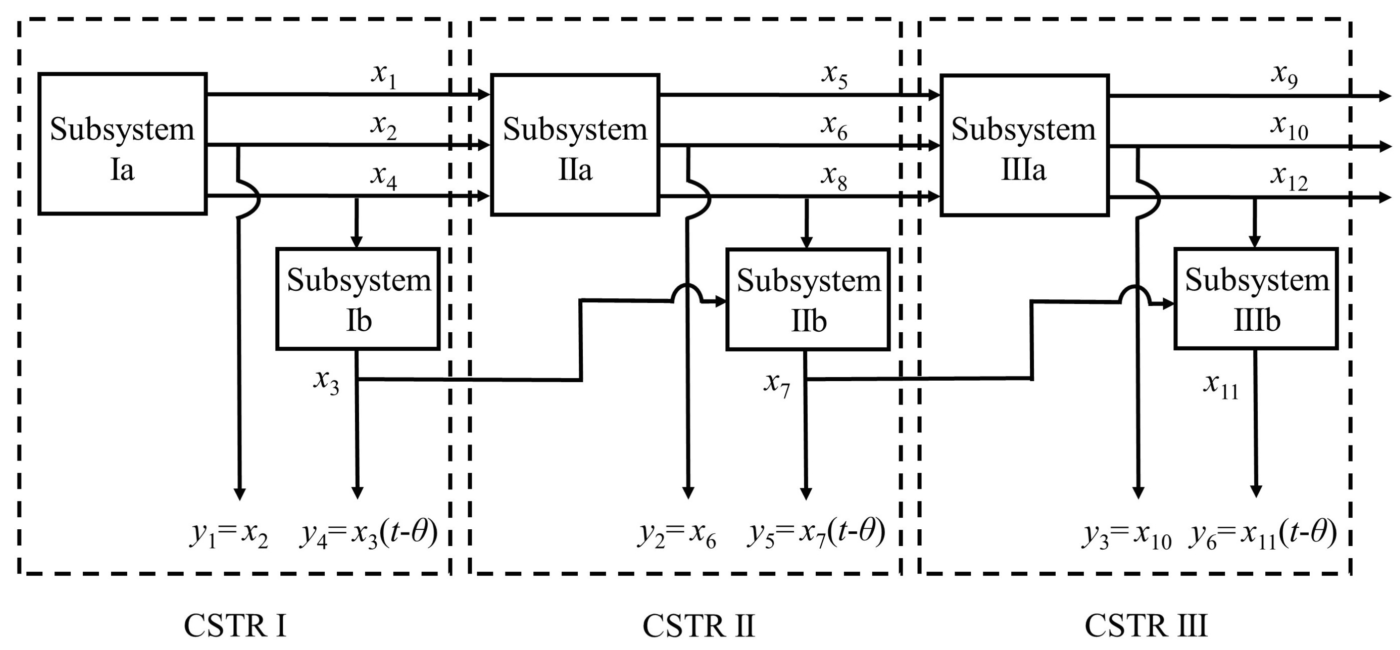
Linear observability analysis was carried out in two different cases: (i) only hydroxyl end groups (, and ) are continuously measured; (ii) in addition to hydroxyl end groups, carboxyl end groups (, and ) are also measured by using on-line acidimetric titration. In Case (i), the conclusion is that the system is not observable, because carboxyl end groups are “downstream” relative to the hydroxyl end groups. It should be noticed that the interfacial concentration of EG does not depend on the state variables in the reactor. In Case (ii), the system of CSTRs is observable. The results of observability analysis suggest that the carboxyl measurement is necessary for accurate estimation of the states and, therefore, of DP, and it should be utilized in the observer despite its low sampling rate.
From a physical point of view, the system of CSTRs clearly possesses a serial structure: the outflow of the preceding reactor is the feed for the next reactor. Thus, it is straightforward to design sequential observers by taking advantage of the particular LBT system structure (as described in
Section 2.2). The interconnection of these subsystems is shown in
Figure 4, from which the unobservability in the absence of carboxyl measurements is clearly visible.
Figure 4.
Subsystems representation of three CSTRs in series.
Figure 4.
Subsystems representation of three CSTRs in series.
4.1. State Estimation with Continuous Measurement Exclusively
In Case (i), the output vector
represents the concentrations of hydroxyl end groups in the reactors, which are continuously measured. Even though the entire system is unobservable in the absence of carboxyl measurements, if only Subsystems Ia, IIa and IIIa are taken into account, the new system becomes observable. In other words, the concentrations of EG and ester groups can be estimated by using only hydroxyl measurement. For the specific system (
i.e., Ia, IIa and IIIa), we have implemented observer Equation (9) with state-dependent gain computed from Equation (10), where the mapping function
is a solution of the system of PDEs of Equation (11) with design parameters
A and
B. Two different choices of the
A-matrix, with different sets of eigenvalues, are used in the simulations: “fast” (−2.0, −1.8, −1.6, −1.4, −1.2, −1.0) and “slow” (−0.2, −0.18, −0.16, −0.14, −0.12, −0.1). Truncation order N = 3 is used considering the balance between the accuracy of the approximate PDE solutions and computation time. The initial guess of the estimates is given in
Table 3.
Table 3.
Initial estimated values for the observer.
Table 3.
Initial estimated values for the observer.
| CSTR# | [EG] (mol/L) | [COOH] (mol/L) | [Z] (mol/L) |
|---|
| CSTR I | 1.0 × 10⁻³ | 7.57 × 10⁻³ | 10.0 |
| CSTR II | 0 | 1.01 × 10⁻² | 10.0 |
| CSTR III | 1.6 × 10⁻³ | 1.13 × 10⁻² | 10.1 |
As a result of being “downstream” states, carboxyl dynamics are detached from Subsystems Ia, IIa and IIIa. An open-loop observer is used to estimate the concentrations of carboxyl end groups, because their dynamics are open-loop stable. The open-loop observer equations are given as follows:
with
,
and
obtained from the observer equations driven by the continuous measurements
,
and
.
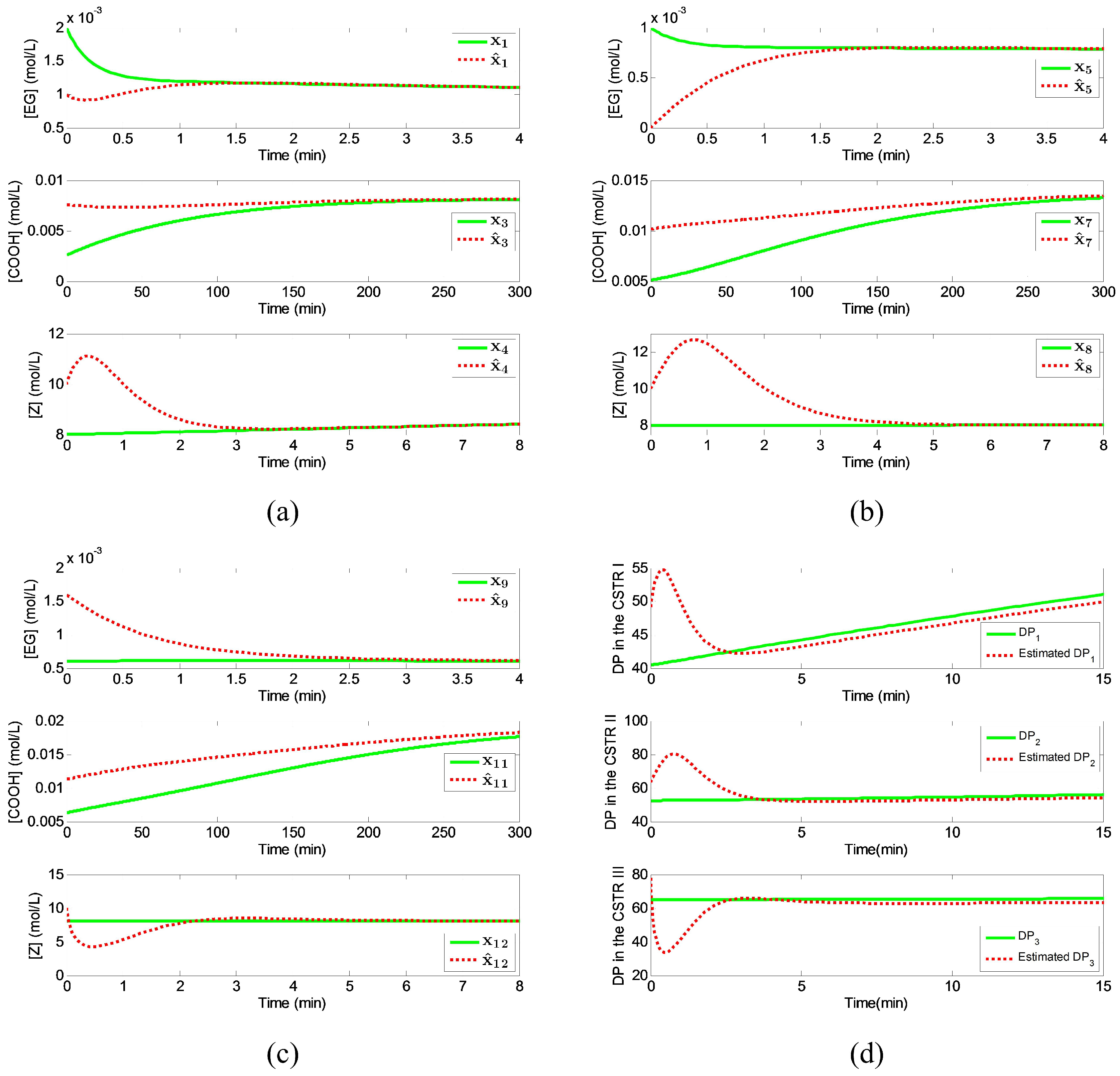
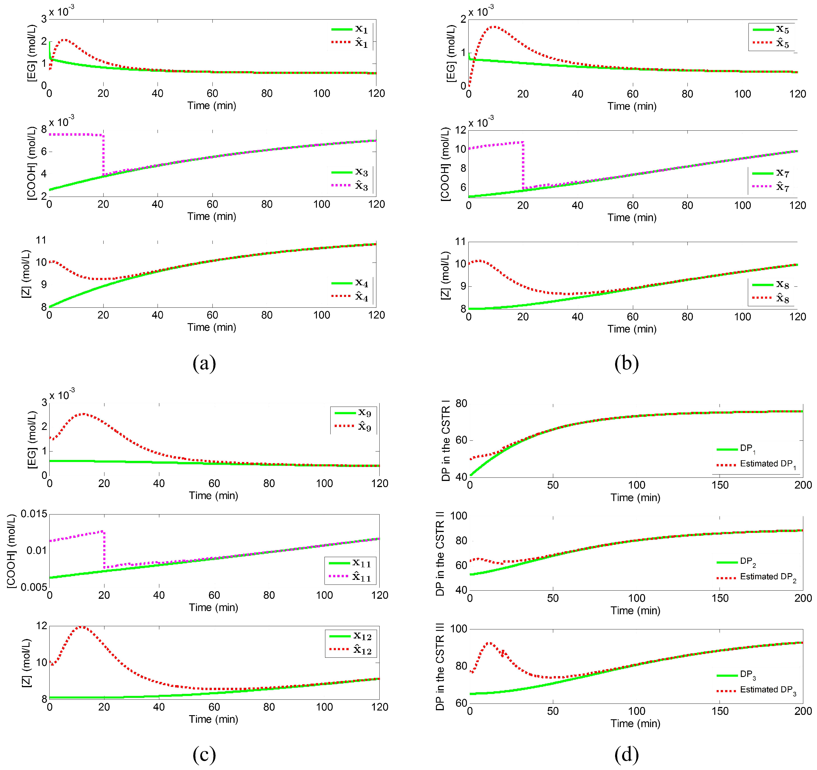
Figure 5 shows the performance of the reduced-order observer with “fast” eigenvalues by comparing the actual and estimated states, as well as DP in the three CSTRs. As a result, the concentrations of EG and ester groups converge to the actual states very fast. Since the unobservable states (
i.e., concentrations of carboxyl end groups) are estimated from an open-loop observer, the speed of convergence depends on the dynamics itself, which is not adjustable. Therefore, it takes much longer to converge. This also explains the offset in the DP estimates in the beginning. However, this offset will be eliminated eventually as
,
and
converge.
Figure 5.
Performance of the reduced-order observer with “fast” eigenvalues: (a) actual and estimated states in CSTR I; (b) actual and estimated states in CSTR II; (c) actual and estimated states in CSTR III; (d) actual and estimated degree of polymerization in all three CSTRs.
Figure 5.
Performance of the reduced-order observer with “fast” eigenvalues: (a) actual and estimated states in CSTR I; (b) actual and estimated states in CSTR II; (c) actual and estimated states in CSTR III; (d) actual and estimated degree of polymerization in all three CSTRs.
4.2. State Estimation with Both Measurements
In Case (ii), both continuous and slow-sampled measurements are utilized in the observer design. Instead of using an open-loop observer, an inter-sample output predictor is used to estimate the evolution of the slow-sampled output during the sampling interval. Meanwhile, dead time compensation is carried out to account for the time delay between the present time and sensor dead time. For acidimetric titration, it is assumed that there is a ten-minute sampling interval, and the dead time of the sensor is twenty minutes. In this case study, it should be noticed that the output of the predictor does not need to feed into the reduced-order observer because carboxyl concentrations do not affect the other states and are not used in the estimation of concentrations of EG and ester groups. However, they will affect the estimation of DP. In this case, the dead time compensator is actually combined with the inter-sample output predictor, demonstrated as follows:
where the state estimates
,
and
are obtained from the continuous-time observer.
,
and
are the delayed outputs with dead time
θ, while
,
and
are the estimates at the present time, respectively. The three equations are initialized at the most recent measurement at
and run from
to
, where
η is the length of the sampling interval. It serves as a dead time compensator between
and
and also serves as an inter-sample output predictor between
and
. In the first
θ time units of each simulation, an open-loop observer is used for estimating carboxyl end groups, because there is no measurement information available.
In
Figure 6, the convergence speed of EG and ester groups is slow because “slow” eigenvalues are chosen in this case. In the estimates of carboxyl concentrations, several steps are observed, because the slowly-sampled measurement corrects the predictor output when the most recent measurement becomes available each time. In addition, the observer together with the inter-sample predictor and the dead time compensator is able to estimate DP accurately in all three CSTRs.
Figure 6.
Performance of the reduced-order observer with “slow” eigenvalues when using both measurements: (a) actual and estimated states in CSTR I; (b) actual and estimated states in CSTR II; (c) actual and estimated states in CSTR III; (d) actual and estimated degree of polymerization in all three CSTRs.
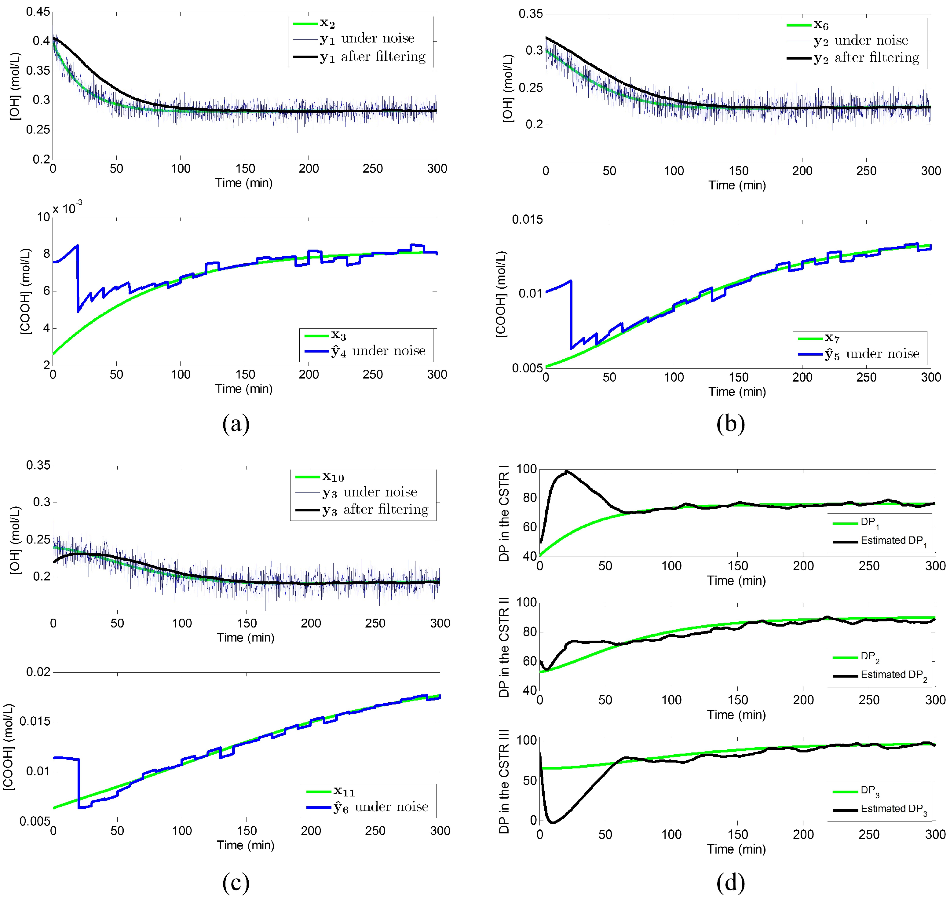
4.3. Observer Performance under Sensor Noise
While the reduced-order observer is computationally more efficient by reconstructing only unmeasured state variables, it suffers from sensitivity to sensor noise. Therefore, the performance of the reduced-order observer needs to be tested under sensor noise. Pre-filtering of the measurement signal may be necessary to cut out the noise, which inevitably introduces some lag.
Figure 7 shows that the same level of white noise is added to all of the hydroxyl measurements with the standard deviation equal to 0.01. A first-order filter is used to cut out the high frequency noise. Different filter factors, 0.005, 0.005 and 0.007, are used respectively according to the filtering needed. As expected, we can see lags in the filtered signal by comparing it to the actual value. White noise with standard deviation
is also considered for the on-line sampled titration measurements.
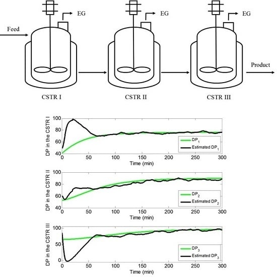
Figure 7d shows both the estimated DP and the actual value when sensor noise is introduced. Fairly accurate estimation is achieved after about 70 min, even though the estimates deviate from the actual states quite significantly in the beginning. Relatively “slow” eigenvalues are used here because “fast” eigenvalues lead to a more aggressive response and may adversely affect observer performance.
Figure 7.
Measurement signals before (blue) and after (black) pre-filtering: (a) in CSTR I; (b) in CSTR II; (c) in CSTR III. Observer performance: (d) actual and estimated degree of polymerization in all three CSTRs.
Figure 7.
Measurement signals before (blue) and after (black) pre-filtering: (a) in CSTR I; (b) in CSTR II; (c) in CSTR III. Observer performance: (d) actual and estimated degree of polymerization in all three CSTRs.


