Development of a Dynamic Model and Control System for Load-Following Studies of Supercritical Pulverized Coal Power Plants

Abstract

Traditional energy production plants are increasingly forced to cycle their load and operate under low-load conditions in response to growth in intermittent renewable generation. A plant-wide dynamic model of a supercritical pulverized coal (SCPC) power plant has been developed in the Aspen Plus Dynamics® (APD) software environment and the impact of advanced control strategies on the transient responses of the key variables to load-following operation and disturbances can be studied. Models of various key unit operations, such as the steam turbine, are developed in Aspen Custom Modeler® (ACM) and integrated in the APD environment. A coordinated control system (CCS) is developed above the regulatory control layer. Three control configurations are evaluated for the control of the main steam; the reheat steam temperature is also controlled. For studying servo control performance of the CCS, the load is decreased from 100% to 40% at a ramp rate of 3% load per min. The impact of a disturbance due to a change in the coal feed composition is also studied. The CCS is found to yield satisfactory performance for both servo control and disturbance rejection.

1. Introduction

Due to the increased penetration of renewables into the electric grid, traditional thermal power plants are being forced to cycle their load and operate under low-load condition to meet changing load demands. However, these plants were designed for neither frequent cycling nor sustained low-load operation. Load-following and part-load operation can lead to considerable losses in efficiency, adverse impacts on plant health, and increases in emissions. To reduce the undesired effects of load-following and part-load operation, advanced control strategies can be helpful for maintaining key controlled variables in their desired range. For developing advanced controllers and studying their performance, a dynamic model of the plant is necessary. Since the model needs to run reasonably fast and achieve desired accuracy, the trade-off between model fidelity and computational expense is an important consideration. For supercritical power plants, an additional computational difficulty is the high degree of nonlinearity in steam properties, especially when the plant transitions between the supercritical and subcritical regimes during load-following.

While there is a large body of literature on dynamic modeling and control of subcritical pulverized coal plants [1], there are fewer studies on supercritical pulverized coal (SCPC) plants. Existing literature on dynamic modeling of SCPC plants can be largely grouped into two categories―those that have focused on individual equipment items and those that have focused on plant-wide model development. The key equipment items that affect the dynamics under load-following operation are those in the boiler section, steam turbine section, and feedwater heater (FWH) section. The existing literature focused on these individual sections is discussed first, followed by a discussion on the literature focused on the plant-wide dynamic model development including plant-wide control.

For supercritical boilers, a number of models with varying scopes have been described in the literature. A “non-equal fragmented model” that captures heat and mass transport characteristics along the height of the water wall has been developed [2]. A model for calculating the heat flux distribution and 3D temperature distribution in a supercritical boiler has also been reported [3]. These studies [2,3] focused only on the furnace combustion and water-wall section. However, it should be noted that the dynamics of the overall boiler depend on the other components of the boiler since the boiler feedwater (BFW) passes through the economizer before going to the water wall. The economizer dynamics, in turn, depend on the dynamics of the superheaters, attemperators and reheaters since the flue gas passes through these sections before entering the economizer. Furthermore, the BFW gets heated in the FWHs before being fed to the economizer. Therefore, due to the pathways of the flue gas and the BFW/steam, all boiler components and some upstream and downstream components must be simulated together. A dynamic model of a 600 MW supercritical plant was developed and used for studying start-up and dynamic behavior [4]. This model included the economizer, superheater, water circulation pump, and water storage tank. The air flow rate was assumed to be sufficient for complete combustion. Thus, no combustion control system was developed. In power plants, the dynamics of the air side can have considerable impact on the dynamics of water/steam-side components, especially during startup and load-following; therefore, consideration of the air-side dynamics is desired. In this work, all sections of the boiler, including air-side control, are modeled with due consideration of the configuration of a typical SCPC plant.

Several models of the steam turbines (ST) are available in the literature. A nonlinear ST model based on approximations of fundamental equations has been developed [5]. This model used identical turbine models for all turbines stages and was validated with steady-state heat balance data from a commercial turbine unit. However, the operation of the governing stage can be different than other stages. Furthermore, models of the back-end condensing stages should account for the presence of moisture. Another nonlinear mathematical model of a ST for a 440 MW power plant was developed to predict the transient behaviors of the turbine system where the model parameters were estimated by a genetic algorithm [6]. Although this model considered separate sub-models for the high-pressure (HP) and intermediate-pressure (IP) sections, where flow was homogeneous, and later stages of the low-pressure (LP) section, where flow was considered to be heterogeneous in order to detect the presence of moisture it also assumed a constant pressure ratio using a first-order transfer function instead of calculating the actual pressure profile. The turbine efficiency was also assumed to be constant. For ST models intended for load-following studies, three aspects should be captured. First, the models of the governing stage, other non-condensing stages, and the condensing stages should be developed such that they can capture the differences in the performance characteristics of these stages. Second, for the non-condensing stages, the efficiency change under load-following operation should be included because of the sliding-pressure operation in SCPC plants and the large variation in the inlet temperature profile that may occur during load-following and low-load operation. Third, the assumption of a fixed number of condensing stages may not always be valid under load-following operation, especially under low-load condition where the reheat temperature may not be maintained at the desired value. Thus, the model should be capable of detecting moisture, if present, in the stages that may be non-condensing under nominal condition. If moisture is present, then the moisture fraction is the variable of interest at the outlet rather than the temperature, which remains constant at the saturation temperature for a given pressure. This change in variables resulting from phase transition can lead to computational issues in a simultaneous equation solver and must be handled effectively in a dynamic model. In this work, conducted in Aspen Plus Dynamics® (APD), pressure and enthalpy are calculated at the ST outlet rather than pressure and temperature (non-condensing) or pressure and vapor fraction (condensing). Then, properties calls are made to obtain the vapor fraction and temperature given the pressure and enthalpy. The changed set of variables is found to yield a model that can be solved reliably if a ST stage transitions back-and-forth between pure vapor phase and two-phase operation.

The FWHs play a key role in achieving high power plant efficiency. An optimal configuration of the FWH network was proposed for increasing the efficiency of a coal-fired power plant [7]. This work considered only high-pressure FWHs as a part of regenerative heating but neglected low-pressure FWHs. For evaluating the performance of FWHs, a nonlinear correlation among the terminal temperature difference, drain cooler approach, and temperature rise was developed as a function of load [8]. However, the extraction flow rate was considered as self-regulating, whereby there is no control valve and the steam flow adjusts itself by a thermal equilibrium process. In another study, a thermodynamic optimization of the heat transfer in the FWHs and exhaust flue gas heat recovery system of SCPC plants was proposed to increase plant efficiency and reduce CO₂ emissions [9]. That work was based on the assumptions of constant pressure ratio in the turbine stages, constant turbine efficiency, constant drain cooling approach, and constant temperature rise. It should be noted that under sliding-pressure operation during load-following, extraction pressure can change considerably leading to control limitations and changes in the condensation temperature of steam, which, in turn, affects the dynamics of the other sections. In this paper, a model of the entire FWH network including a regulatory control layer is developed and included in the plant-wide model so that its impact during load-following operation can be studied.

Works on plant-wide dynamic models and control of SCPC plants in the existing literature are very few in comparison to the works on coal-fired subcritical power plants [10,11]. Recently a comprehensive review of dynamic modeling of thermal power plants was provided [12]. A dynamic model of an SCPC power plant developed in the process simulation software Apros® was used to investigate operational flexibility and transient behavior. Under sliding-pressure operation, the load was decreased from 100% to 27.5% in six steps in 185 min, a ramp rate of 0.4%/min [13]. Energy utilization in a 660 MW SCPC power plant under load-following condition has been studied using a model developed in the GSE software [14]. The GSE model was used to study energy-saving opportunities during load-following by considering a typical coal consumption rate. A 50% load change under sliding-pressure mode was obtained with a maximum ramp rate of 0.5%/min. The ramp rates considered in both these studies are far below the cycling demands and current industrial practices of about 3–8% load change per minute [15]. In addition, none of these studies included the industry-standard coordinated control system (CCS) that is essential to study the dynamics of operating plants. 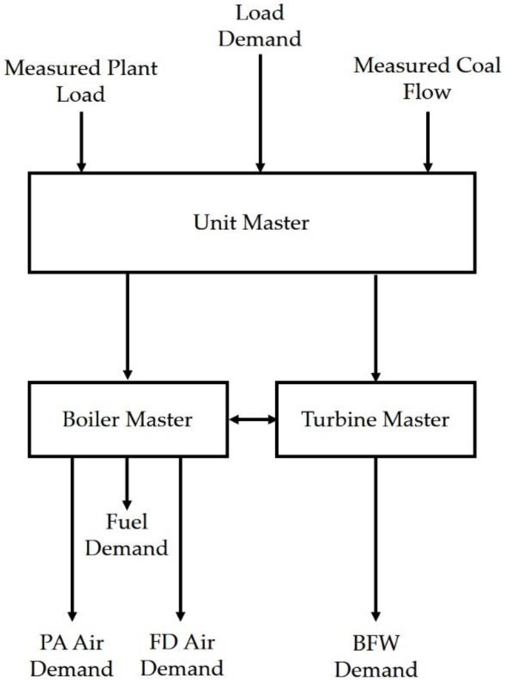Recently, another dynamic model of an SCPC power plant was developed in Apros® and validated against steady-state and transient plant data [16]. The ramp rates studied in this paper are in an industrially acceptable range of 3–8% load per minute. However, few details about the control configuration, except for the load control and main steam temperature control, were provided. Also, no disturbance rejection studies were conducted. During rapid load-following operation, careful consideration must be provided for not only the dynamics of the main steam temperature but also the dynamics of the reheat steam temperature, since they affect both the plant efficiency as well as the extent of condensation in the last few turbine stages, which affects ST health. Furthermore, developing the plant-wide control system requires simultaneous consideration of the FWH section, boiler section, and the ST section due to strong interactions among these sections. The CCS including the FWH control is necessary for plant-wide control. In this paper, a CCS is designed and its performance for load-following is studied. It should be noted that the CCS presented here does not represent or reproduce that of any vendor or any power plant but was developed by the authors based on the information available in the open literature and control requirements under load-following operation.

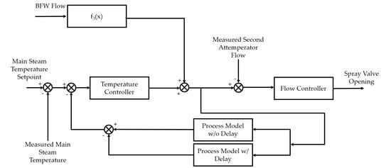
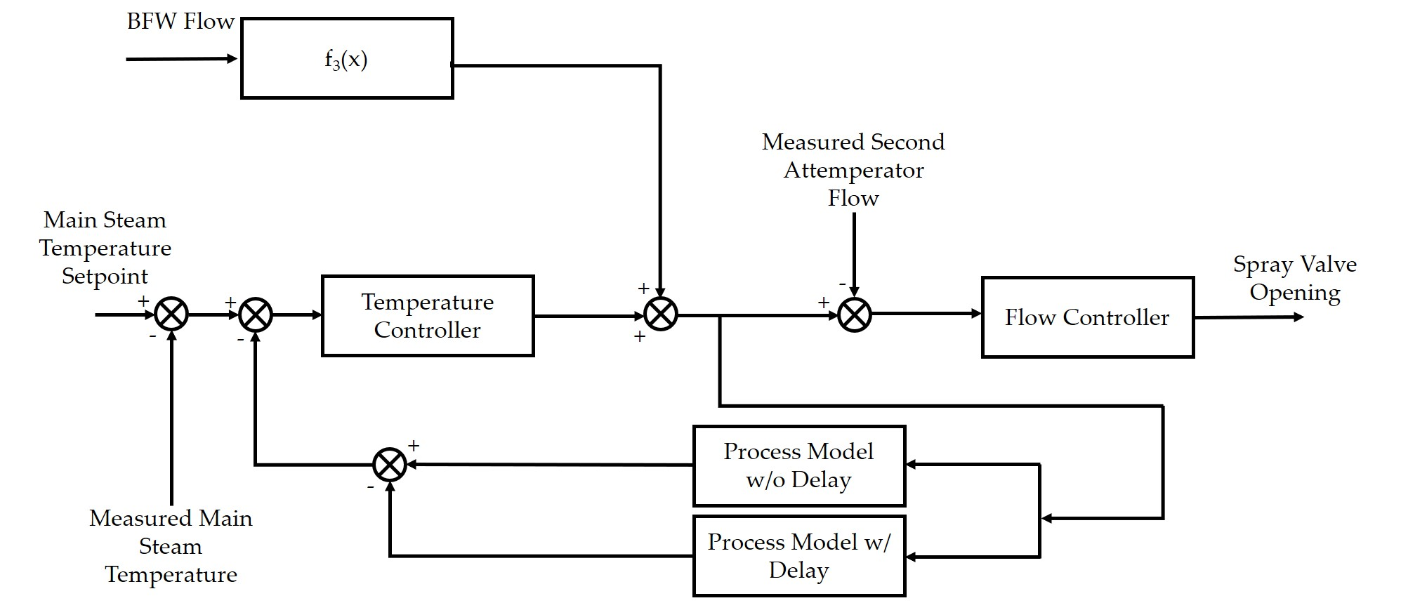
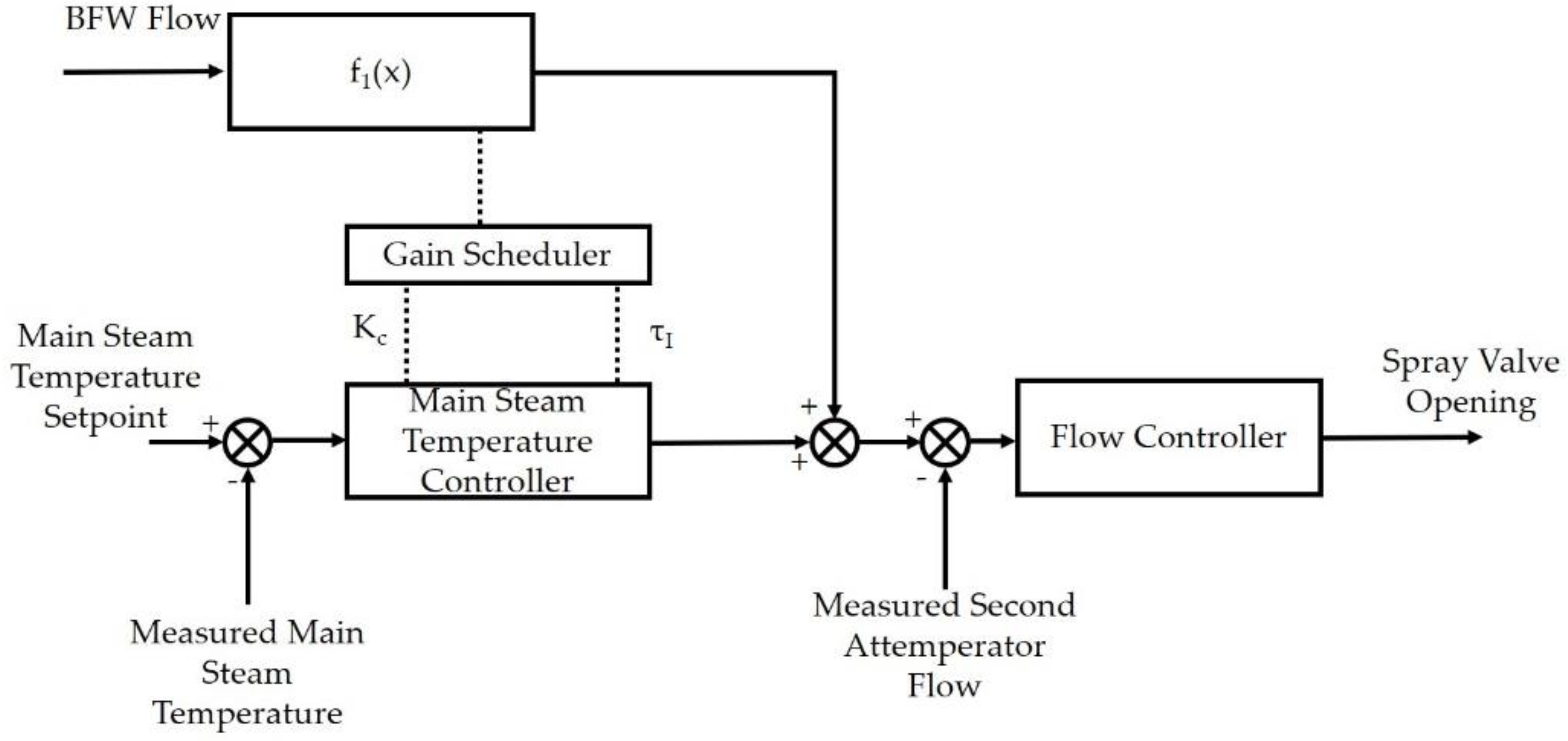
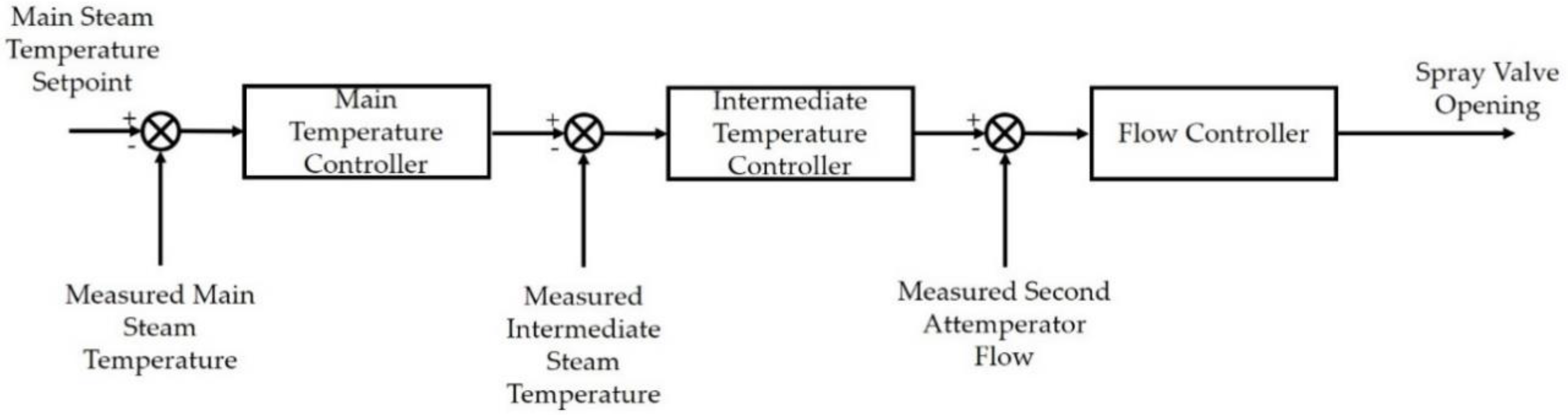
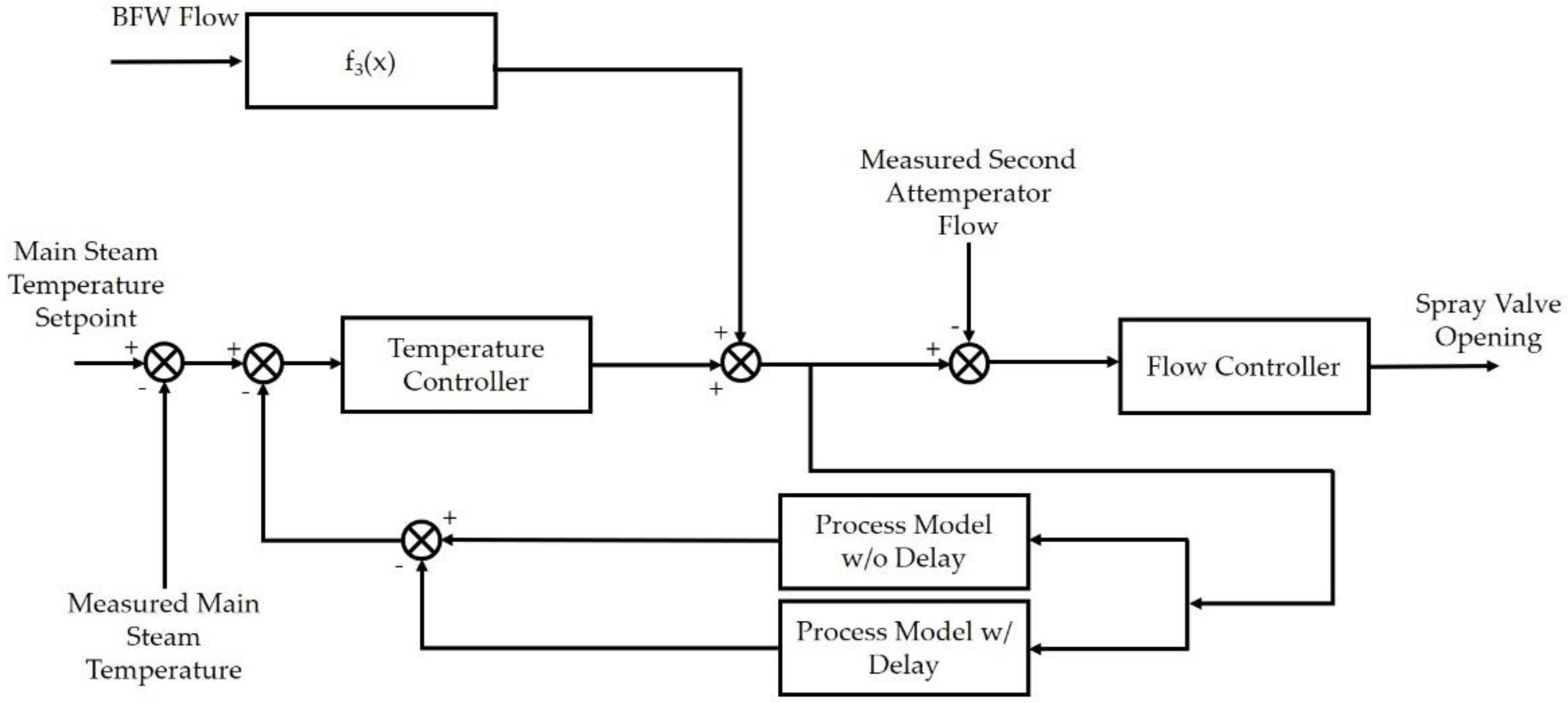
In this work, first a steady-state model of an SCPC power plant is developed. The configuration and nominal operating conditions of the plant are similar to Case B12B (for a 550 MWe net SCPC plant using Illinois No. 6 coal) from the cost and performance baseline study by the National Energy Technology Laboratory (NETL) [17]. The steady-state model is developed using Aspen Plus® (AP) and ACM then converted to a pressure-driven APD model, where the regulatory control layer and CCS are developed. Tight control of the main steam temperature is desired under load-following condition, since a lower temperature leads to losses in efficiency, and a higher temperature can lead to damage in the superheater tubes in the boiler and the leading stage(s) of the turbine. While the fire side of the boiler has very fast dynamics, the steam-side dynamics are comparatively slower due to the considerable thermal holdup in the boiler tubes. Due to considerable time delay, tight control of the steam temperature under load-following operation becomes challenging. For the main steam temperature control, a Smith predictor for time-delay systems is developed and implemented as part of the overall CCS in addition to traditional strategies in power plants for steam temperature control. For evaluating the performance of the CCS, the plant load is ramped down from 100% to 40% at 3% load change/min under sliding-pressure operation. The remaining sections of this paper are arranged as follows. Section 2 provides details of the SCPC power plant configuration and dynamic process sub-models. Section 3 describes the design of the control system. Section 4 provides the simulation results followed by the conclusions in Section 5.

2. Process Sub-Models

2.1. Plant Configuration

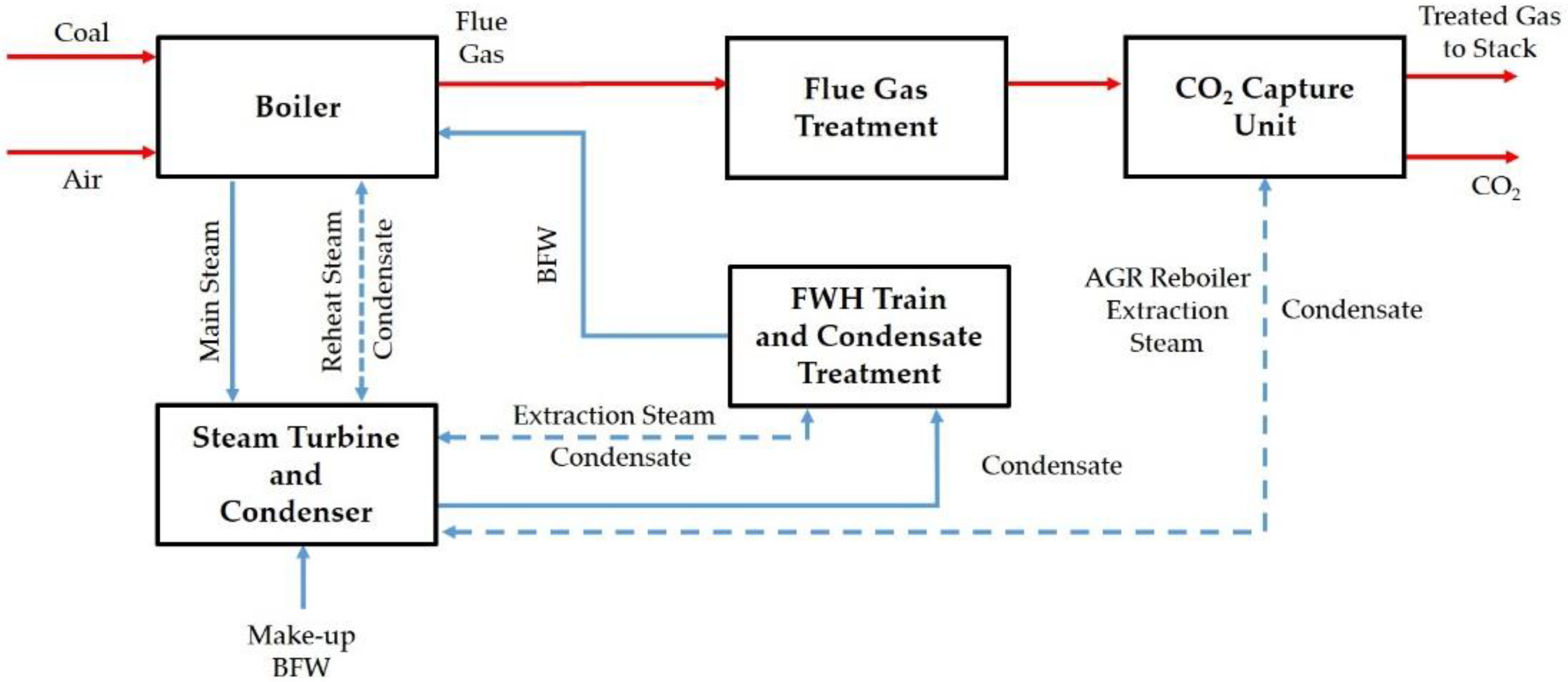
The SCPC power plant configuration presented consists of a once-through steam boiler with flue gas treatment and a supercritical steam cycle with single steam reheater. There are four main sections: the feedwater treatment and heating sections, the supercritical boiler section that includes air fans as well as the air preheater, the ST section, and the flue gas treatment section, including some consideration for acid gas recovery (AGR). The configuration of the plant is shown in Figure 1, as adapted from the NETL study [17]. The referenced configuration also includes CO₂ capture, but a detailed model of that section is not included in the current study. Nevertheless, the steam extraction for the AGR section was modeled to correctly characterize the power produced in the ST; these extraction flows were assumed to change proportionally with load. Another important note is that the coal feed in Figure 1 is located after the coal pulverizers, which were not considered as part of this study. It should also be noted here that the double-ended arrows indicate extracted steam flowing for use as a heating medium and the then-cooled effluent returned to the surface condenser in the ST section.

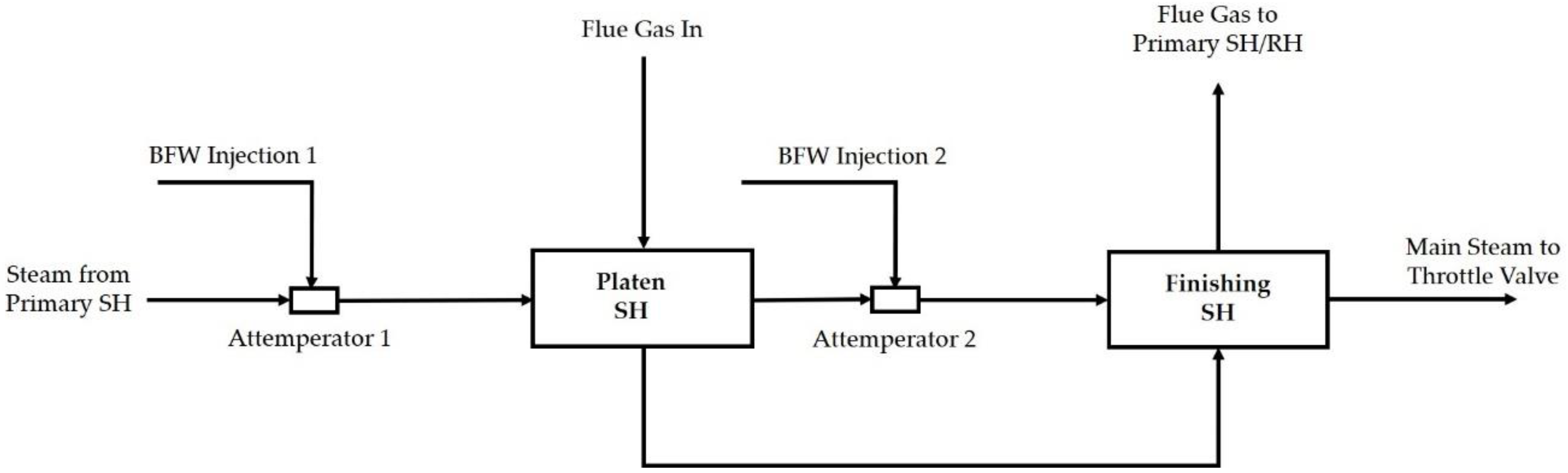
In the boiler, pulverized coal is combusted producing hot flue gas. The boiler section consists of various components including an economizer, water wall, separator, reheater, multiple superheaters, two-stage attemperation for the main steam, and one-stage attemperation for the reheated steam. In the steam cycle, the supercritical steam at 593.3 °C and 241.2 bar is sent to a HP turbine, where it is expanded to 47 bar in three stages. The expanded steam is then returned to the boiler where it is reheated to 593.3 °C, before it is sent to a three-stage IP turbine and subsequently to the five LP turbines. To enhance the overall power cycle efficiency, steam is extracted from the turbines for feedwater heating.

The dynamic SCPC model in the APD software was generated by first developing a valid pressure-flow network in the steady-state SCPC model in the AP software. This modeling task required connecting the pressure nodes in the SCPC plant through flow nodes that relate pressure drop with volumetric flow rate [18]. In dynamic simulations, specification of equipment sizes, their geometries, and orientations are crucial for capturing the transient behavior of the system. Volumetric holdup in equipment items affects the rate of accumulation, which is one of the key factors that determines the transient response [18]. Each of the vessels was sized based on its steady-state operating conditions, and these geometrical details were used in the APD model; in dynamic simulation this allows for the dynamics to be captured relative to the nominal condition and provides the most logical basis for equipment design. The dynamic SCPC model operating at base load was shown to be in good agreement with the steady-state results from the NETL baseline study [17].

Specific component lists with appropriate physical property packages were assigned to the individual sections of the plant as necessary in order to accurately capture the interactions in each section based on local components and conditions. This helped to minimize the zero-flow components in specific streams and equipment models, thereby improving solver convergence properties and reducing computational time.

2.2. Feedwater Heaters

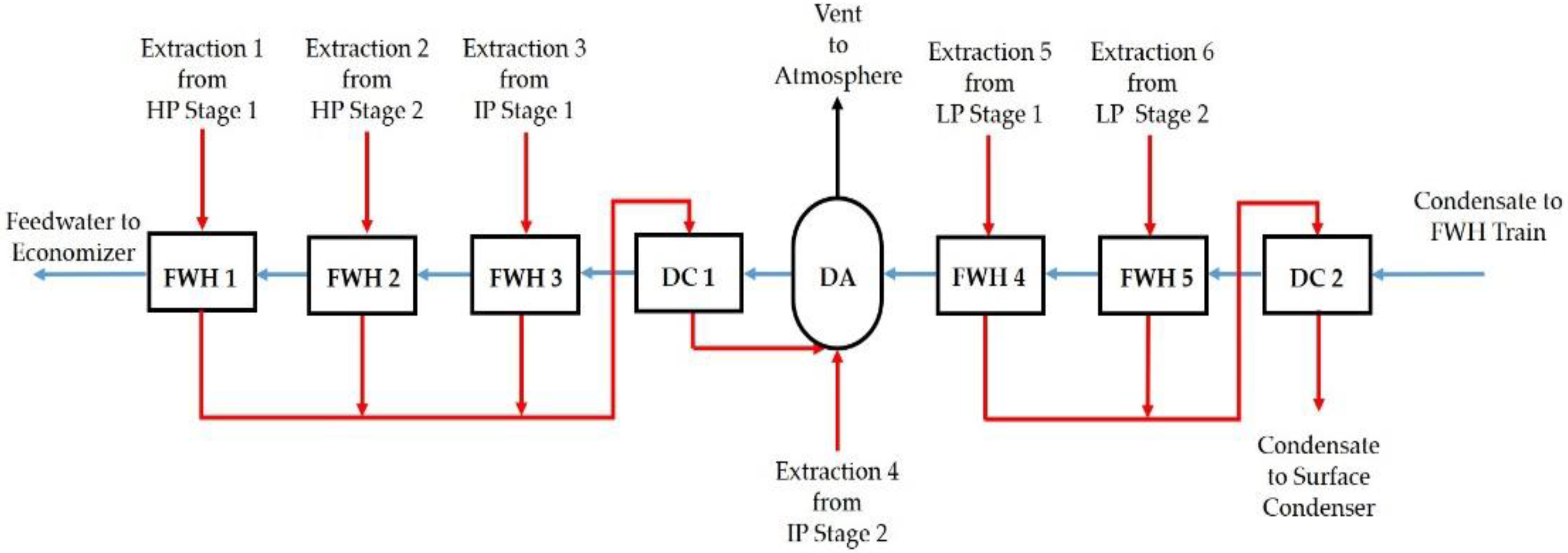
Figure 2 shows the layout of the feedwater pretreatment and heating section of the SCPC plant with, one deaerator (DA) and seven total exchangers consisting of five FWHs and two drain coolers (DCs) [17]. The main difference between the FWHs and the DCs is that in the FWHs heating is accomplished primarily using the latent heat from the extracted steam, whereas in the DCs the sensible heat of the condensate from the FWHs is used for heating the feedwater. Extracted steam from HP Stage 1 and HP Stage 2 is fed to FWH 1 and FWH 2, respectively, with an extraction from IP Stage 1 fed to FWH 3. The condensate from these three FWHs is sent to DC 1 and subsequently to the deaerator. In the deaerator, extracted steam from IP Stage 2 is used for removing dissolved oxygen. Extracted steam from LP Stage 1 and LP Stage 2 is fed to FWH 4 and FWH 5, respectively. The condensate from these two FWHs is sent to DC 2 and subsequently to the surface condenser.

Aspen Exchanger Design and Rating (EDR) was used to size each of the FWHs as a shell-and-tube heat exchanger based on its steady-state operating conditions. Aspen EDR sizes heat exchangers based on a constrained optimization, accounting for the process conditions within an economic framework [19]. Sizing information for the FWHs including the volumes and metal masses of the shells and tube bundles was used in the APD models. For more information on the Aspen library models, interested readers are referred to several resources available in the public domain [18,20,21,22,23,24].

2.3. Simplified Boiler Model

As noted above, gas-side dynamics of SCPC boilers are very fast in comparison to the water/steam side. Additionally, the flue gas has a low density and heat capacity in comparison to the water/steam in SCPC plants. For comparison, the ratio of the product of specific enthalpy and density (characterizing the thermal holdup) for water/steam to gas is more than 500 under conditions at the water-wall of the boiler. Therefore, in this work, gas-side dynamics have been neglected, and the gas side is assumed to be instantaneous. The ultimate analysis of the coal provided in

Table 1. Ultimate Analysis of Coal Feed to the Boiler.

Component	Weight %
H2O	11.12
C	63.75
H2	4.50
N2	1.25
Cl	0.29
S	2.51
O2	6.88
Ash	9.7

is the same as that for the Illinois No. 6 coal in the NETL baseline study [17].

The following sections of the boiler are modeled with due consideration of thermal and volumetric holdup: economizer, water wall, primary superheater, platen superheater, finishing superheater, and reheater. Typical inlet and outlet temperatures of the water and flue gas in these sections are estimated based on the NETL study [17], information available in the open literature [25], and the results of an energy balance.

The flue gas exiting the boiler section is sent to the flue gas desulfurization (FGD) unit. Since this work primarily focuses on the dynamics of the front end of the power plant, models of back end sections like the flue gas treatment section are very simple. A simple stoichiometric reactor with 98% conversion of SO₂ was developed for the FGD section where the SO₂ in the flue gas reacts with lime slurry to form calcium sulfite that is then oxidized with air to form gypsum. The flue gas finally leaves the system via the carbon capture unit.

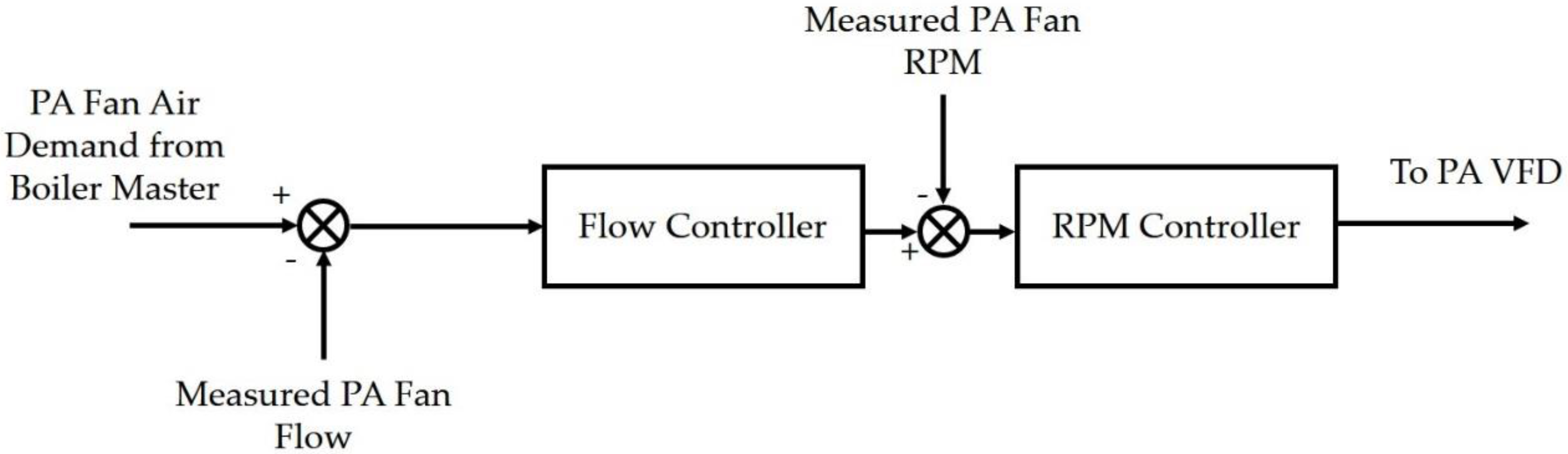
2.4. Fan Models

The primary air (PA) and forced draft (FD) fans are used for providing air to the pulverizers and burners in the boiler, respectively. During load-following operation of the plant, changes in these air flow rates affect the energetics in the boiler and the auxiliary power requirements. Therefore, the control system needs to be designed appropriately. For large power plants, the PA and FD fans are typically operated by variable frequency drives (VFDs) that modulate the fan speed to obtain the desired flow rate. Since fan curves that represent the head and power with respect to flow rate at various revolutions per minute (RPMs) are not currently available for the FD and PA fans corresponding to this work, an approximate method is developed. A family of curves available in the open literature [26] for similar sized fans is scaled to match the desired range of head and flow. Then, a quadratic function between the head and flow is regressed to the family of curves simultaneously where each regression coefficient is considered to be a linear function of RPM.

2.5. Steam Turbine

Three separate ST models were considered to capture the operating characteristics of the various stages of the ST:

• Leading (Governing) Stage
• High-Pressure (HP), Intermediate-Pressure (IP), and Low-Pressure (LP) Stages
• Final Stage before Condenser

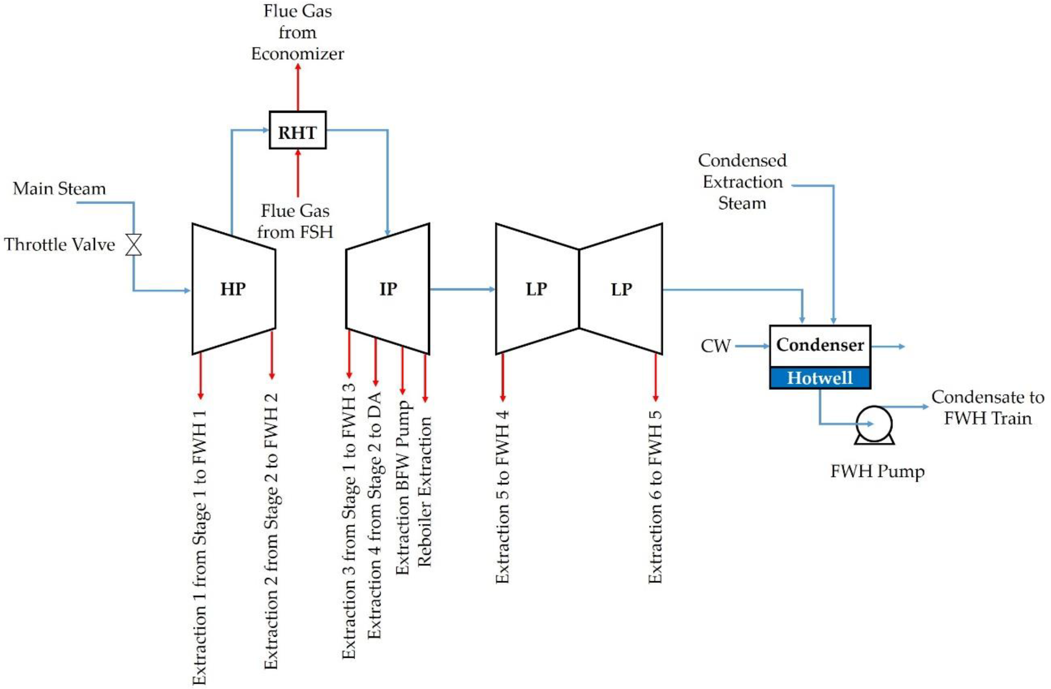
Figure 3 shows the layout of the turbine section of the SCPC plant [17]. The main steam from the finishing superheater of the boiler is throttled and fed to the governing stage of the HP turbine. There are three physical stages in the HP section. Extractions 1 and 2 from the first and second stages of the HP turbine section are sent to FWHs 1 and 2, respectively. After the HP section, steam is heated to 593 °C under the nominal condition by returning it to the boiler through a single reheater followed by attemperation. The reheated steam is sent to the IP section of the turbine that comprises two physical stages. Extractions 3 and 4 from the first and second IP stages, respectively, are sent to FWH 3 and the deaerator, respectively. After the IP turbines there are auxiliary extractions connected to various reboilers and a single turbine for auxiliary equipment, and the steam goes to the LP section that comprises five physical stages, with two extractions to FWHs 4 and 5, after LP stages 1 and 2, respectively. The effluent steam from the final LP stage is then fed to a surface condenser where it is condensed with cooling water (CW). The condenser is integrated with a hotwell from which the FWH pump returns water to the feedwater treatment and heating section.

Each of the turbine stage sub-models described below was developed in ACM. These custom models were then compiled into library blocks and used in the steady-state model in AP. The same blocks were used in APD to build a model for the entire ST, including extractions and auxiliary equipment items. The isentropic power generated by any given turbine stage without condensation is given by Equation (1), where the power for the condensing stage is shown later.

$$\mathcal{P}= {\eta }_{is}M\Delta h_{is}$$

(1)

Turbine dynamics are fast and, therefore, have been neglected in this model. Turbine dynamics can be important during plant startup/shutdown, but those operations are not considered in this work.

2.5.1. Leading Stage

The leading stage model was considered separately for two reasons: capturing the change in the leading stage efficiency under extremely nonlinear property changes and considering the control setups for fixed-pressure operation [27]. For fixed-pressure operation, separate governing valves are used in the control of separate arcs of admission into the turbine. Here, an array of four instantiations of the model are used to represent the true leading stage at the nominal condition. In each model instance, the flow, $M$, through the stage is calculated by Equation (2), where the flow parameter C_flow is designed for the nominal load. The efficiency, ${\eta }_{is}$, of the leading stage is then calculated using Equations (3) and (4). The equations used for this model are adapted from the work of Liese [27].

$$M= C_{flow}\frac{P_{in}}{\sqrt{T_{in}}}\sqrt{\frac{\gamma }{\gamma -1}\left[{\left(\frac{P_{out}}{P_{in}}\right)}^{\frac{2}{\gamma }}-{\left(\frac{P_{out}}{P_{in}}\right)}^{\frac{\gamma +1}{\gamma }}\right]}$$

(2)

$$V_o=\frac{44.72}{W}\sqrt{(1-R)(h_{out}-h_{outi})}$$

(3)

$${\eta }_{is}=2\left(\frac{V_{rbl}}{V_o}\right)\left[\left(\sqrt{1-R}-\frac{V_{rbl}}{V_o}\right)+\sqrt{{\left(\sqrt{1-R}-\frac{V_{rbl}}{V_o}\right)}^2+R}\right]$$

(4)

2.5.2. HP, IP, and LP Stages

The model for all the stages between the leading and last stage models is a thermodynamic stage-by-stage model [28]. Here, a model that represents a single thermodynamic stage was developed and then repeated as needed to represent the boundaries of each section with extractions placed at the appropriate pressure levels. The HP, IP, and LP sections are comprised of seven, fourteen, and seven thermodynamic stages, respectively.

For the thermodynamic stages, the isentropic efficiency, ${\eta }_{is}$, is correlated with the specific shaft speed, N_s, as seen in Equations (5)–(7). The other important parameter in these calculations is the isentropic head parameter, k_is, which is used for calculating the total enthalpy change as shown in Equation (8). Here, the calculation is made for each stage at the nominal operating condition via Equation (9) and then the value remains fixed during dynamic simulation. These equations are adapted from the work of Lozza [28].

$$\Delta ef= -0.0049{(ln\left|N_s+0.001\right|)}^3-0.031{(ln\left|N_s+0.001\right|)}^2-0.060(ln\left|N_s+0.001\right|)-0.022$$

(5)

$$ef=0.072{(ln\left|N_s+0.001\right|)}^3+0.020{(ln\left|N_s+0.001\right|)}^2-0.010(ln\left|N_s+0.001\right|)+0.89$$

(6)

$${\eta }_{is}=ef(1-\Delta ef)-0.87(1-f_v)$$

(7)

$$\Delta h_{is}=\frac{k_{is}{u}_{mv}^2}{2W}$$

(8)

$$k_{is}=2.2+8.9e^{-43N_s}$$

(9)

Accounting for moisture is essential in calculating the actual power produced by a given stage. The existence of moisture also significantly affects the efficiency of the stage. As noted earlier, if moisture is present, then the model needs to calculate moisture fraction as opposed to temperature, which becomes fixed. A logic-based approach for detection of moisture based on the dew point calculation and subsequent structural changes, if moisture is present, does lead to convergence issues during load-following since APD uses an equation-oriented approach. The change in solving from pressure and temperature to pressure and vapor fraction yields a discontinuous system about the dew point, creating the convergence problems. One way of avoiding the logic-based approach is to change the variables from temperature or vapor fraction to enthalpy. Thus, while pressure and temperature fully define the system in absence of condensation, and pressure and moisture fraction fully define the system under condensation, pressure, and enthalpy fully define the system for both presence and absence of condensation. This change in variables avoids issues with structural changes in an equation-oriented framework.

2.5.3. Final Stage

The modeling of the final turbine stage is important since this stage typically operates under a choked flow condition, and it has different performance characteristics than other stages. In addition, due to condensation in this stage under typical operating conditions, the stage efficiency calculation needs to be modified [27]. The Stodola equation (Equation (10)) is considered to represent the flow through this stage in the presence of condensation. The exit pressure of the last stage is constrained to the pressure of the surface condenser, which is again affected by the cooling duty of the condenser. Equations (11) and (12) show the calculation of the end-line end-point and the used-energy end-point enthalpies; these enthalpies correspond to the calculation of the efficiency for this stage by accounting for the generation of moisture. Then efficiency is calculated from Equations (13) and (14). The power produced by the condensing stage is shown by Equation (15) as a function of the real enthalpy drop accounting for the presence of moisture. Here, these equations are adapted from Liese [27], as follows:

$$M= C_{flow}\frac{P_{in}}{\sqrt{T_{in}}}\sqrt{1-{\left(\frac{P_{out}}{P_{in}}\right)}^2}$$

(10)

$$h_{elep}=h_{in}+(h_{is}-h_{in}){\eta }_{dry}{f}_v(1-0.65f_l)$$

(11)

$$h_{ueep}=h_{elep}+TEL{\eta }_{dry}{f}_v(1-0.65f_l)$$

(12)

$$\Delta h_r=h_{in}-h_{ueep}$$

(13)

$${\eta }_{is}=\frac{\Delta h_r}{\Delta h_{is}}$$

(14)

$${\mathcal{P}}_{cond}= M\Delta h_r$$

(15)

3. Control System Design

As mentioned earlier, the water-side of the SCPC system is a time-delay system that makes the design of the control system challenging. In addition, steam properties and heat transfer characteristics are highly nonlinear as the system transitions from the supercritical to subcritical region or vice versa during load-following. Furthermore, the highly complex configuration of the FWHs, coupled with the sliding-pressure operation that changes the pressure of the steam extractions, leads to considerable further challenges in the control system design. In SCPC power plants, a coordinated control system is usually used for load-following [29]. The CCS is implemented as the supervisory layer that exploits the regulatory control as degrees of freedom to achieve the control objectives during load following.

3.1. Regulatory Control Layer

The regulatory control layer is developed using the minimum amount of control needed for dynamic convergence. It consists of 16 single-loop feedback controllers and 13 cascade control loops, where proportional-integral-derivative (PID) controllers are used. A few of these controllers are discussed in detail below. Under the nominal condition of the SCPC plant, phase separation does not take place in the separator that is located between the water wall and primary superheater. Therefore, under the nominal condition, the inventory on the water side is controlled in the hotwell and in the deaerator. The deaerator level is maintained by manipulating the incoming BFW flow rate while the hotwell level is maintained by manipulating the demineralized water flow rate to the hotwell, under the assumption that a condensate storage tank can be neglected.

As mentioned earlier, maintaining the reheat temperature while following the load is important. A lower temperature than desired will lead to efficiency losses and higher condensation in the LP turbine section. A higher temperature than desired will lead to damage in the superheater tubes and turbine. Typically, at the vertical downpass of the boiler, the flue gas is split between the reheater and primary superheater. The flue gas split fraction going to the reheater section can be modulated by a damper to help control the reheat temperature. In addition, the BFW flow rate to the attemperator, located after the reheater, also assists in the reheat temperature control.

3.2. Supervisory Control Layer

As noted before, the typical supervisory control layer for SCPC plants is the CCS, which helps to follow the load with due consideration of the synergies between the boiler and turbine and interactions among the manipulated and controlled variables, as laid out briefly in the literature [29]. Figure 4 shows the overall CCS master diagram that has been developed in this work and implemented in APD. While the required coal flow rate for a desired power output can be calculated based on the calorific value of the coal and the overall system efficiency, the system efficiency changes under load-following operation. Therefore, the heat rate correction is considered while calculating the trim to the boiler master and the turbine master inputs. It should be noted here that there are various functions and ratios implemented in the control systems described below. For simplicity, these functions are represented only in the form f(x) in the control diagrams for main steam temperature control in Section 3.4 and BFW flow control in Section 3.5.

3.3. Air Flow Rate Control

Figure 5 and Figure 6 show the control diagrams for the two fans that supply air to the boiler: the forced draft (FD) fan and the primary air (PA) fan, respectively. In the SCPC plant, the PA fan supplies air to the pulverizers transporting coal to the burners. Here, the air through the pulverizers is accounted for to accurately model the system interactions even though the pulverizers are not explicitly modeled. Based on the output signal of the boiler master controller, set points for air flow for the PA and FD fans are calculated. The corresponding set points for fan speeds in RPM are sent to the respective fan VFDs that modulate the frequencies to obtain the desired RPMs, based on the performance curves explained in Section 2.4. The VFD control is represented by a simple PID controller. For the FD fan, a trim is provided based on the oxygen concentration in the boiler outlet flue gas. Proper control of the excess oxygen is crucial in that, if the excess oxygen drops too low, incomplete combustion might result leading to a process safety risk; if it becomes higher than needed, the higher heat loss through the exiting flue gas from the system would reduce the boiler efficiency.

3.4. Main Steam Temperature Control

As mentioned before, tight control of the main steam temperature is desired for maintaining efficiency during load following. Furthermore, large deviations in the main steam temperature can lead to undesired creep and fatigue in the boiler tubes and turbine components. Temperature of the main steam is controlled by attemperation using BFW spray at two locations: the first immediately before the platen superheater (SH) and the second immediately before the finishing SH as shown in Figure 7. Here, the second attemperator plays the key role in controlling the main steam temperature by regulating the spray flow, while the first attemperator assists by ensuring that the second attemperator spray is within a set range of operation, leaving room for changes in response to disturbances or fast load changes.

Three configurations for main steam temperature control are investigated here, where the manipulated variable is the BFW flow rate injected into Attemperator 2. Configuration 1 and Configuration 2 are typical control strategies reported in literature [10]. Configuration 3 is the strategy proposed in this work, with comparisons of the three strategies to follow in the results.

3.4.1. Configuration 1

Configuration 1, shown in Figure 8, consists of a simple feedback loop with a feedforward correction based on the steam flow rate [10]. As discussed before, large excursions in the main steam temperature should be avoided. However, there are considerable nonlinearities in the steam properties especially during transitions between the supercritical and subcritical regions. A gain-scheduled controller is used in Configuration 1 to help improve control for this nonlinear system. The feedforward term helps to improve the disturbance rejection characteristics of the loop.

3.4.2. Configuration 2

In Configuration 1, temperature of the main steam is controlled without any consideration of the intermediate steam temperature immediately after Attemperator 2. The temperature of this intermediate steam responds faster to changes in the BFW spray flow rate in comparison to the main steam temperature, which lags due to the thermal and volumetric holdup of the finishing SH. In Configuration 2, the intermediate steam temperature controller manipulates the BFW injection flow rate to Attemperator 2 as shown in Figure 9 [30]. The PID controller that is used for the main steam temperature control generates the set point for the intermediate steam temperature controller. It should be noted that this configuration does not consider any feedforward correction.

3.4.3. Configuration 3

As noted before, there is significant time-delay in the water/steam side of the SCPC plant. For closed-loop stability of such systems, a smaller gain has to be used in the PID controller leading to sluggish response that is undesired for main steam temperature control. One classic approach for control of a time-delay system is the Smith predictor [31]. For designing the Smith Predictor, the finishing SH is represented as a first-order process with time-delay as follows [31]:

$$y\left(s\right)=\frac{K_c{e}^{-\theta s}}{{\tau }_s+1}\times u(s)$$

(16)

A minor feedback loop is introduced in the conventional feedback structure, along with a feedforward compensation. The block diagram for the Configuration 3 control scheme developed in this study is shown in Figure 10.

3.5. BFW Flow Control

Figure 11 represents the control diagram for the BFW flow control. The BFW flow plays a key role in achieving sliding-pressure operation and ensuring that the temperature constraints at various locations of the boiler can be satisfied. The BFW flow rate set point is load-dependent and corrected via the enthalpy at the water wall (WW) outlet in the boiler and by the degree of attemperation as shown in Figure 11 [32]. A trim is also provided based on the water wall outlet enthalpy, that can be calculated based on the water wall outlet temperature and pressure. The CCS determines the load-dependent set point for the BFW controller based on the turbine master output signal. The trim, which is based on the opening of the main steam Attemperator 1 valve, ensures that the Attemperator 1 valve opening retains sufficient gain to move this system in response to sudden load changes.

4. Results

Table 2. Steady-State Validation for Full Load.

Parameter	Unit	NETL Baseline Study	SCPC Model	Error
Coal Flow Rate	tonne/h	225	228	1.53%
Gross Power	MW	641	620	−3.28%
Net Power	MW	550	532	−3.21%
Heat Rate	kJ/kWh	11,086	11,629	4.90%
Main Steam Pressure	MPa	24.2	24.1	−0.37%
Main Steam Temperature	°C	593	593	0.00%
Main Steam Flow Rate	tonne/h	2003	2027	1.19%

compares the results of the simulation at full-load condition for the SCPC plant-wide dynamic model developed in this study and the steady-state NETL baseline study [17].

Using the CCS detailed above, transient studies were conducted on the response of the SCPC plant to ramp changes in power demand (load). Here, the studies were conducted for a load decrease from 100% to 40% over 20 min, corresponding to a ramp rate of 3% load per min. This ramp rate is within an acceptable range of power industry ramp rates while maintaining all key operating variables within allowable deviations from their set points. A near-perfect tracking of the load was accomplished (not shown here). During these studies, each of the configurations detailed above were used in turn, and in the following results their responses are either shown explicitly or deemed similar to one another and discussed as such.

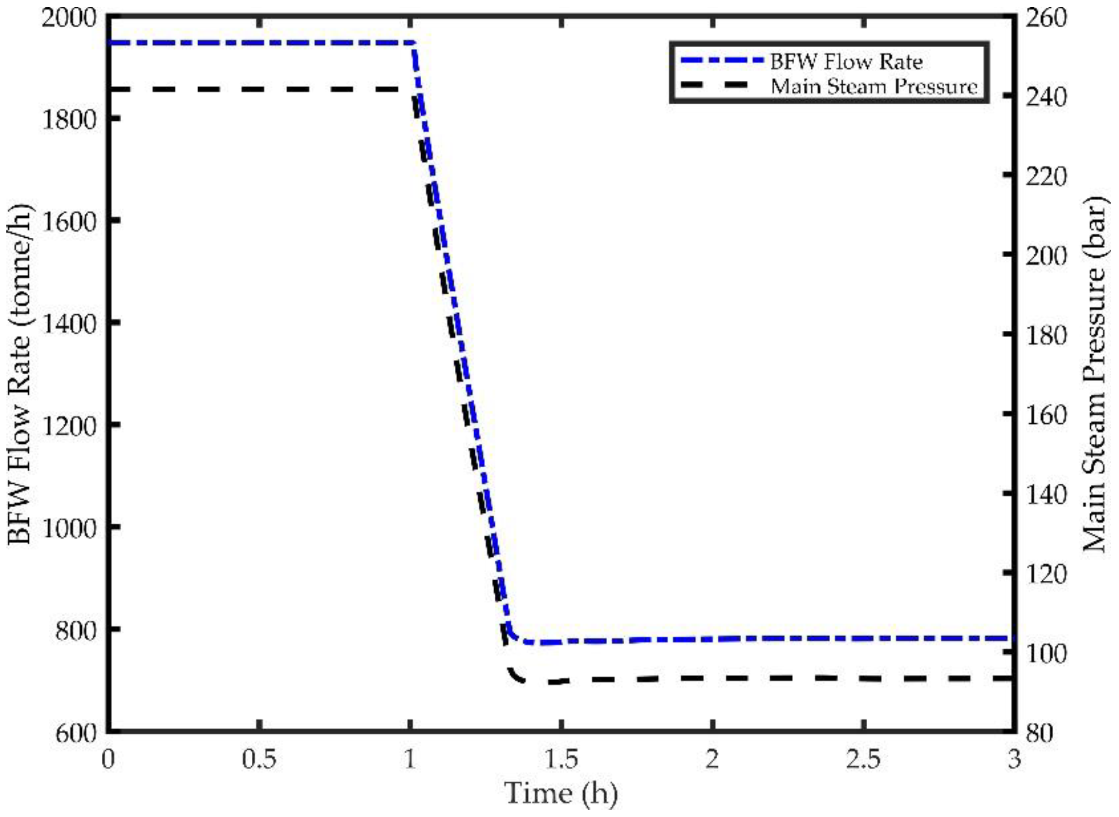
Figure 12 represents the response of the BFW flow rate and the main steam pressure to the 60% ramp down in load starting at time equal to 1 hr. The BFW flowrate and main steam pressure decrease by approximately 63% and 62%, respectively. These responses are hardly affected by the main steam temperature control figurations. The main steam pressure slides from 242 bar to 93 bar, corresponding to a ramp rate of 7.5 bar per min.

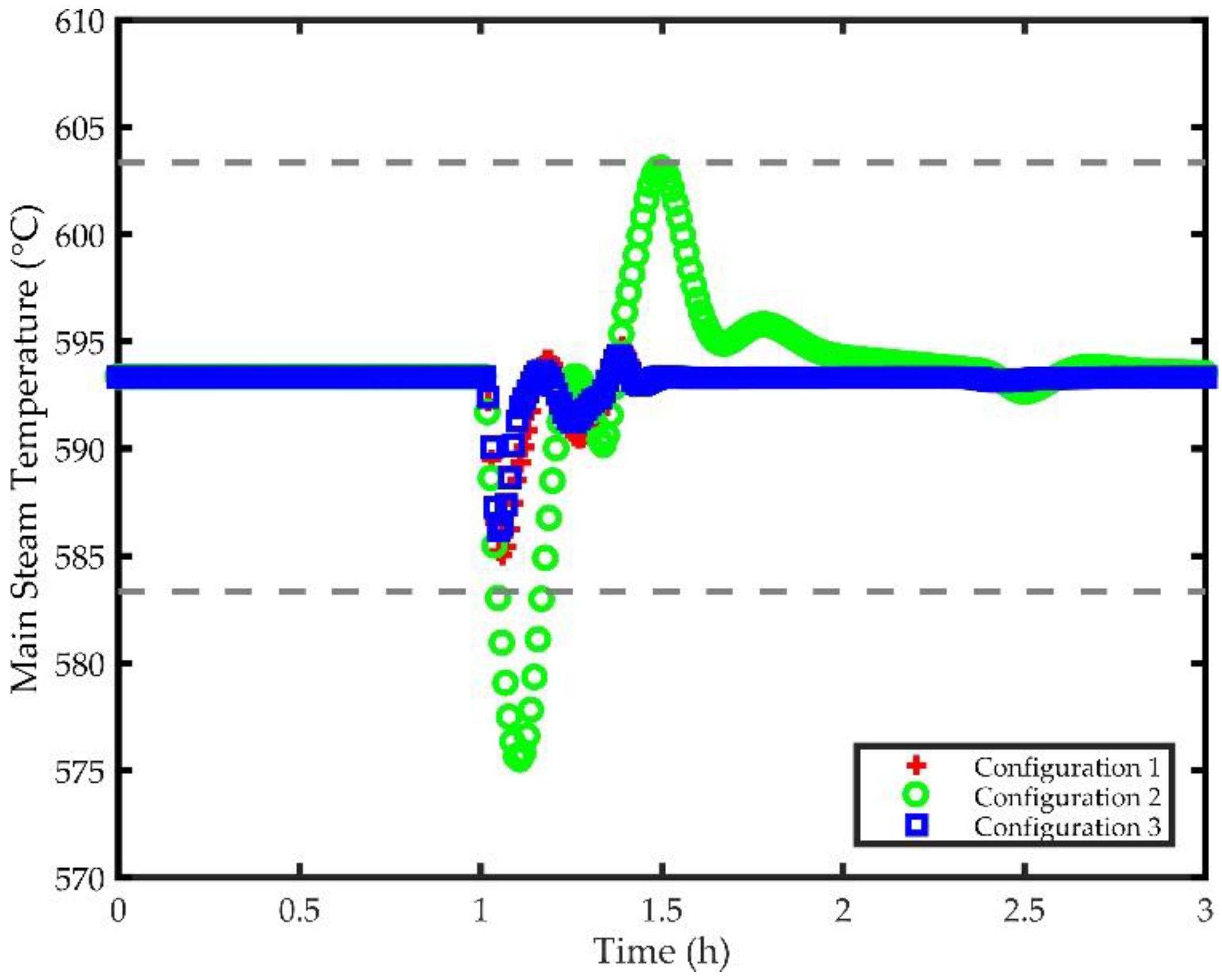
Figure 13 depicts the response of main steam temperature to the 60% reduction in load for each of the control configurations detailed above. A ±10 °C band shown in Figure 13 is considered to be the acceptable range. Both Configurations 1 and 3 lead to main steam temperatures that are well within the band; however, Configuration 2 results in a large undershoot that is unacceptable because of boiler efficiency losses, ST efficiency losses, added thermal stresses on the reheater, and added condensation in the trailing LP stages, leading to damage to the ST. The large undershoot of about 18 °C Configuration 2 comes from a lack of accounting for the dead time in the system, leading to a controller that is out of sync with the system dynamics and thereby has to catch up with the system. Configuration 3 provides the best control performance, limiting the maximum deviation in the main steam temperature to about 7 °C and resulting in a settling time of about 15 min following the end of the ramp down in load. Configuration 3 is the best performer, due to the characterization of the dead time by the Smith predictor, though the control performance of Configuration 1 is similar.

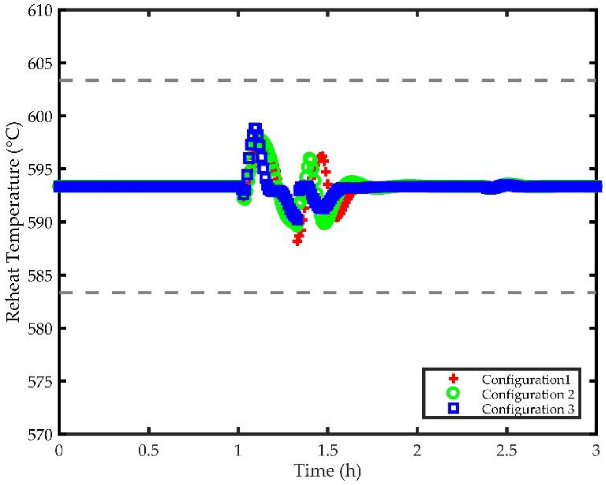
Figure 14 shows the response of using attemperation after the reheater to control the temperature of the reheated steam returning to the IP turbine. Impacts of the three control configurations, that were similar to the main steam temperature control, are shown in Figure 14, with the bands representing deviations of ±10 °C. It can be seen here that the reheat temperature could be brought back to the original set point by each of the configurations considered. Though Configuration 3 has slightly higher overshoot than Configurations 1 and 2, it has faster settling time and lower oscillation. The performance of Configuration 1 is found to be the worst. However, the performance of each configuration is acceptable for controlling the reheat steam temperature.

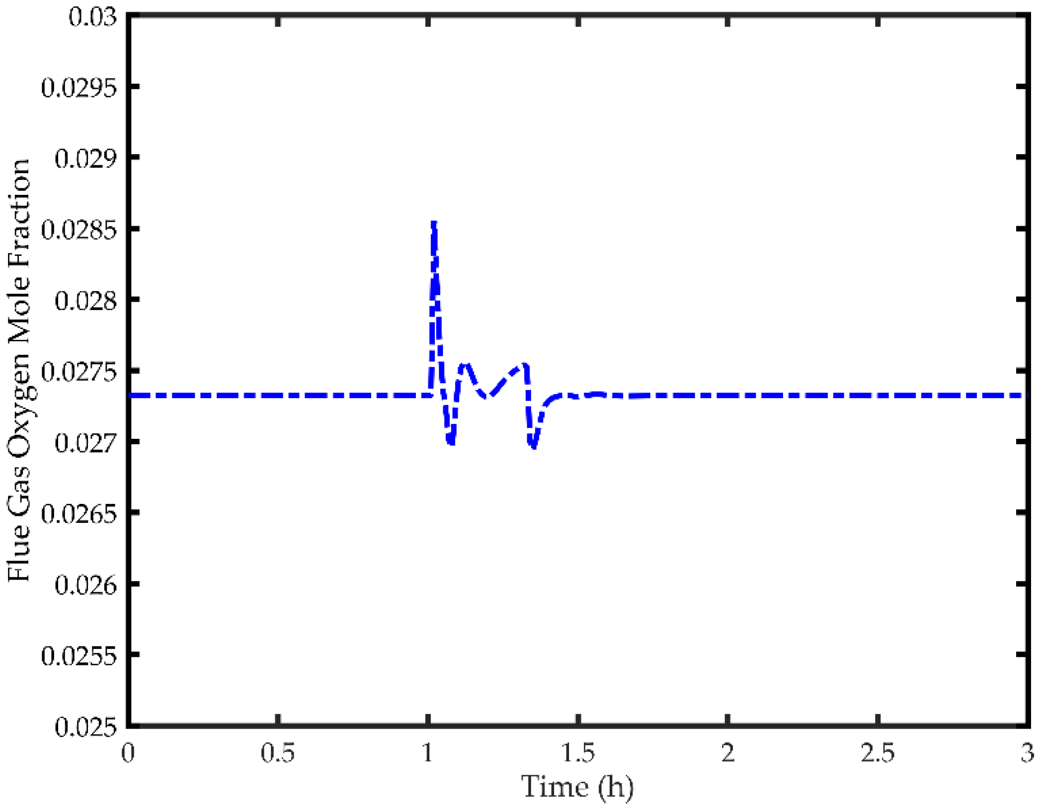
Finally, Figure 15 represents how the oxygen concentration in the boiler flue gas outlet responds to the 60% ramp decrease in load. Here again, the configuration used for main steam temperature control has no effect on the response of the oxygen concentration so only one plot is shown. It can be seen in Figure 15 that the maximum deviation in oxygen concentration is within ±5%.

The composition of coal fed to a power plant can change considerably. The CCS should be designed for rejecting this disturbance efficiently while maintaining a set load. The base case composition of Illinois No. 6 coal shown in Table 1 is changed as shown in

Table 3. Comparison of Coal Compositions for Disturbance Rejection Study.

Ultimate Coal Analysis
	Base Case	Changed
H2O	11.12	13.18
C	63.75	59.36
H2	4.5	5.18
N2	1.25	1.49
Cl	0.29	0.29
S	2.51	2.88
O2	6.88	7.92
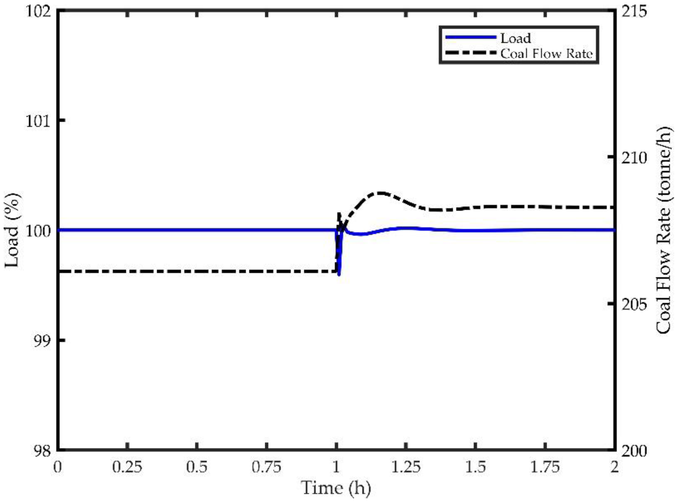
Ash	9.7	9.7

for this transient study, corresponding to 2.59% reduction in the calorific value of the coal feed. This change is centered around expected deviations in coal composition, even when considering coal of a similar grade or from the same mine. Here, it can be observed that the calorific value of the coal can deviate over a range of feeds, a disturbance that the CCS must be able to handle.

Figure 16 shows the transients in load and coal flow for the change in coal feed composition at time equal to 1 h. Here, because of the lower calorific value of the new coal, the load drops by approximately 0.4%, leading to an increase in the coal feed to compensate. Note that the results are only shown here for using Configuration 3 to control the main steam and reheat steam temperatures, given similarities across the results for the three control configurations.

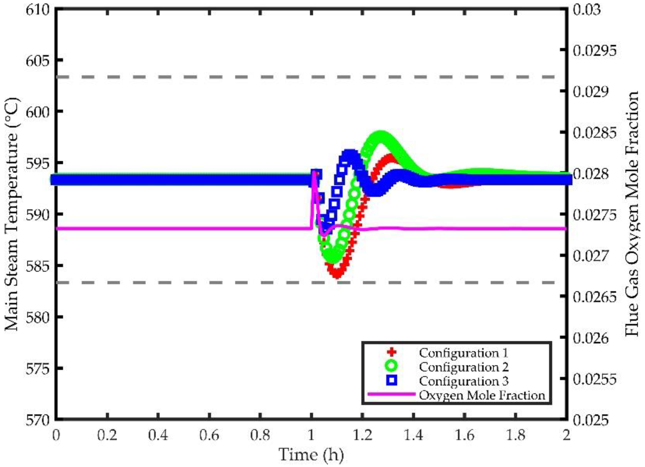
Figure 17 shows the transients in the main steam temperature and flue gas oxygen concentration in response to the disturbance in coal composition. Here, again, a ±10 °C band is set on the main steam temperature. It is observed that Configuration 2 has lower undershoot (about 8 °C) than Configuration 1 but has higher overshoot than Configuration 1 (about 5 °C). Configuration 3 results in considerably lower under/overshoot with a maximum deviation of about 5 °C. Configuration 3 also results in a settling time that is more than 20 min faster compared to other configurations. Irrespective of the configuration for steam temperature control, the oxygen concentration remains relatively constant at its setpoint as shown in Figure 17.

5. Conclusions

A plant-wide dynamic model of a supercritical pulverized coal power plant with CO₂ capture is developed in this work. A coordinated control strategy is designed and its performance is studied for both servo control and disturbance rejection. Sliding-pressure operation is considered while ramping down the load from 100% to 40% at a ramp rate of 3% load per min. As the main and reheat steam temperatures must be controlled tightly, performance of three control configurations is evaluated. For main steam temperature control Configuration 3, which includes the Smith predictor for handling time delays on the water/steam-side, results in maximum deviation of about 7 °C in the main steam temperature and a settling time of about 15 min following the end of the ramp change. Configuration 1 also provides similar control performance. However, Configuration 2 results in a much poorer tracking control performance with the maximum deviation of about 18 °C in the main steam temperature and much longer settling time. For the reheat temperature control, Configuration 3 has the best performance and Configuration 1 has the worst performance while performances of all three configurations are acceptable.

Performance of the control system is evaluated for a disturbance in the coal feed composition. The reduction in the calorific value of the coal feed could be rejected very efficiently by the coordinated control strategy. Maximum deviation in the load is found to be about 0.4% when the coal calorific value was changed by about 2.6%. Maximum deviation in the main steam temperature is found to be about 9 °C, 8 °C, and 5 °C for Configuration 1, Configuration 2, and Configuration 3, respectively. Settling time of Configuration 3 is found to be faster by more than 20 min in comparison to the other configurations. It should be noted that no feedforward input is considered for this disturbance. Overall, Configuration 3 with the Smith predictor is found to provide the best performance for main and reheat steam temperature control for both tracking and disturbance rejection scenarios. Our future work in this area will focus on development of higher fidelity models for various plant components and development of model-based control strategies for further improvement in control performance.