A PSO-Based Recurrent Closed-Loop Optimization Method for Multiple Controller Single-Output Thermal Engineering Systems

Abstract

For solving the problems of closed-loop optimization on controller parameters of multiple-controller single-output thermal engineering system, this paper proposes a recurrent optimization method that is based on the particle swarm computing and closed-loop simulation (PSO-RCO). It consists of a set of closed-loop identification, simulation, and optimization functions that are organized in a recurrent working flow. The working flow makes one controller tuned at a time whilst others keep their values. It ends after several rounds of overall optimizations. Such a recurrently alternative tuning can greatly speed up the convergence of controller parameters to reasonable values. Verifications on practical data from a superheated steam temperature control system show that the optimized control system performance is greatly improved by reasonable controller parameters and practicable control action. With the advantage of not interfering system operation and the potential supporting on big data identification method, the PSO-RCO is a promising method for control system optimization.

1. Introduction

Proportional-Integral-Derivative (PID) control is the most classic control strategy and still the mainstream in thermal engineering control at present [1]. Due to the characteristics of thermal engineering system, such as large range of load variation, long-term continuous operation, nonlinear dynamics, and multiple disturbances, the control performance of PID controller may become worse in operation, resulting in large fluctuation and deviation of process states and jeopardizing the safe and economic conditions of the process. Therefore, PID parameters need retuning from time to time for adapting to varying working conditions.

There are two essential ways for optimizing PID parameters, i.e., the open-loop method and closed-loop method. The open-loop method needs to add a step variation on manipulated variables to an open-loop controlled process and may affect production negatively, therefore it cannot be used for frequent PID parameter tuning. On the contrary, the closed-loop optimization method works on closed-loop control system and does not interfere with process states, thus it could be a more suitable way for controller parameter optimization.

There are two classes of closed-loop PID-parameter tuning methods. One is the conventional method such as the critical proportional band method, the attenuation curve method, the single parameter self-tuning method and so on [2]; another one is the intelligent computing (IC)-based parameter optimization method. Evolutionary multi-objective optimization algorithms with Particle Swarm Optimization (PSO), Genetic Algorithm (GA) and Bacteria Foraging Optimization are used respectively to tune PID controller parameters in [3] and compared with the conventional Ziegler Nichols method, showing the best performance by PSO. GA is adopted for tuning PID parameters in an application of electrical furnace temperature control and the Integral of Absolute index is used for assessment [4]. In [5], the PID-PSO, Fuzzy-PSO, and GA-PSO are taken respectively for improving the speed control of dual star induction motor and the Fuzzy-PSO behaves the best. Genetic Programming is studied for the PID parameter tuning in [6]. In [7], a comparative study on the reactive nature-inspired algorithms for PID controller tuning is taken and it reaches that PSO is the best algorithm. It is easy to understand that the conventional method is appropriate for a single controller, but not convenient for multiple-controller loop according to its working principle [8].

However, thermal engineering processes are often complex, including multiple variables, multiple disturbances, coupled control loops and so on. The conventional closed-loop method cannot handle these issues in control parameter tuning. The IC-based closed-loop control parameter optimization method is able to handle these conditions, because IC algorithms like PSO is good at solving complex optimization problems, especially in hyperspace. There are some examples for using IC to tune controller parameters. The genetic algorithm is used in [9] to design PI parameters but only for a boiler-turbine model. The particle swarm algorithm is used in [10] to optimize the inner-loop PI parameters of a cascaded superheated-steam-temperature control system, while the outer loop is not optimized but upgraded with a kind of advanced controller. When there are multiple controllers to be set in a system, it is usually difficult for IC algorithm to converge quickly to the optimal solution due to the large number of parameters of multiple controllers. Moreover, unreasonable or infeasible controller parameters are apt to appear in optimization results due to coupled relationship among multiple controllers in a single-output system. Therefore, there are still big problems in applying the IC-based closed-loop control parameter optimization method to the field.

In order to solve the aforementioned problems, this paper proposes a PSO-based recurrent closed-loop optimization method (PSO-RCO) for multiple controller parameters in a single-output thermal engineering process. There are many multiple-controller single-output systems in thermal engineering processes, e.g., the superheated-steam-temperature control system which often has 2–4 controllers in single or cascaded loops for regulating the outlet steam temperature of superheaters in boiler-turbine units. In modeling, a multiple-controller single-output system should be described as a multiple-input-and-single-output (MISO) expression. The superheated steam temperature is always influenced by many factors, e.g., steam flow, desuperheated water flow and upstream steam temperature [11]. It also has large inertia due to long tube volume. These all bring about control problems for steam temperature [12]. Because superheated steam temperature is a critical quantity on unit lifetime, efficiency and load following capability, frequent tuning on its control parameter adapting to circumstances is in need [13]. It is also a persuasive example for verifying the PSO-RCO method.

The major contributions of the paper are summarized as follows.

(1)

A controller parameter optimization approach based on closed-loop identification and simulation is proposed for thermal engineering processes. It takes advantage of field data in history database to identify precise dynamic model for optimizing practicable controller parameters.

(2)

A recurrent optimization working flow is proposed for tuning multiple controllers and single output system. Comparing to the simultaneous optimization on all controller parameters, it can better avoid unreasonable or infeasible optimization solution due to couplings among multiple controllers in a single-output system.

(3)

Considering multiple disturbances in thermal engineering system, the intelligence computing is considered for the optimization on controller parameter rather than classical tuning methods. The IC-based optimization can find improved practicable controller parameters through operating simulation model with field data inputs.

(4)

Due to efficient optimization ability on multi-dimension real-number problems, the canonical PSO algorithm is adopted for PID parameter optimizing in the approach.

(5)

For an integrated consideration of control performance and control energy cost, the multi-objective fitness function is adopted in PSO.

The rest of the paper is organized as follows. Section 2 presents the whole idea of the PSO-RCO method first and then unfolds details of modeling, simulation and optimization methods involved in PSO-RCO. Section 3 applies the PSO-RCO method on a superheated-steam-temperature control system. Section 4 draws the conclusions.

2. Methodology

The PSO-RCO algorithm is composed of closed-loop identification function, control loop simulation function, PSO parameter-tuning function, and recurrent-optimization monitor, as shown in Figure 1. The holistic working flow is organized by the recurrent-optimization monitor. The major concern of each function and overall working flow will be explained in the following subsections.

2.1. Control Loop Simulation

Since the simulation-based controller parameter optimization requires high similarity to the field system, a high-fidelity simulation model of the control system to be optimized should be established first. The real control strategy for thermal engineering processes is often very complex for dealing with the complicated process dynamics including large inertia, strong coupling, nonlinearity and the like. Besides PID controllers, there are many other auxiliary links in control strategies for feedforward compensation, high and low limitation on manipulated variables, input dead-zone limitation, and noise filtering. All the links applied in field control loops should be included in simulation models. Therefore, the closed-loop simulation model should be built strictly according to the practical control strategy. Another equally important aspect about the simulation accuracy is the similarity of model for describing the dynamic characteristics of controlled plant.

2.2. Closed-Loop Identification on Controlled Plant

The dynamic model of controlled plant should be able to reflect all major measurable influences which are defined as the manipulated variable and disturbance variables. To this end, the MISO model for the controlled plant is adopted and identified by using field data sampled from closed-loop systems. First of all, the selection for appropriate identification samples should keep the following principles [14].

Principle 1.

Persistent excitation on input signals.

There must be some persistent excitation on input signals of the identified plant. Since the variables of a thermal engineering process are strongly coupled, a continuous and obvious load variation can make the input variables of a MISO model varying and the sampled data during this period can meet the requirement.

Principle 2.

Closed-loop identifiability.

The identifiability for a controlled plant of using its closed-loop samples can be supported by any of the following conditions.

(1)

The controlled process has long time delay or large inertia

(2)

There are disturbances in the feedback channel and the inputs and outputs of a plant are measurable.

(3)

The data is sampled from setpoint perturbation processes.

Principle 3.

Linear independence of input signals.

The input signals with noisy measurement of a MISO thermal system can guarantee the linear independence of the input signals which is necessary for dynamic model identification.

Therefore, the closed-loop identification method is suitable for thermal engineering processes with large-inertia or time-delay dynamics, setpoint tracking, and noise-involved measurements.

The following MISO AutoRegressive eXogenous(ARX) model is adopted for identification.

$$y_t=-{\displaystyle \sum _{i=1}^n{a}_i{y}_{t-i}}+{\displaystyle \sum _{p=1}^{n_u}\left({\displaystyle \sum _{j=1}^{m_p}{b}_{p,j}{u}_p{{}_{,}}_{t-j-d_p}}\right)},d_p\ge 0$$

(1)

where y_t denotes the output at time instant t which is the linear combination of the previous output sequence y_t-i with coefficient a_i and the sum of n_u- input linear combination. The pth input linear combination is the sum of inputs u_p,t-j-dp, with coefficient b_p,j, where u_p,t-j-dp is the value of the pth input variable at time instant (t-j-d_p), m_p is the inertia order of the pth input variable, d_p is the time delay of the pth input variable and n_u is the number of input variables. n is the order of output variable, and m_p is often taken the same as n in identification. The format of Model (1) implicates the long time delay denoted by d_p or large inertia denoted by m_p which are required by closed-loop identifiability as stated in Principle 2. When identifying model (1), the structural parameters of order and time delay need to be determined first and then the coefficients.

2.2.1. Auto-Selection of Model Order and Time Delay

The cross-correlation function of each input-and-output channel is computed to identify its pure time delay [15]. The cross-correlation function is given by

$$R_p=\frac{1}{S}{\displaystyle \sum _{j=1}^S\left|u_p(j)y(j+d_p)\right|}$$

(2)

where S denotes the number of samples, $d_p=1,2,\dots ,K_p,K_p\left(<<S\right)$ denotes the maximum of time delay from the pth input to the output. The value of d_p corresponding to the maximum of R_p indicates the pure time delay from the pth input to the output, denoted as d_p,s.

Then using the singular value decomposition (SVD) method based on Hankel matrix [16], one can find the order of model (1). The method is described in the following.

First, the pth (p = 1, n_u) input time series should be right shifted by d_p,s-sampling points according to its output sequence. Second, a sufficient high-order MISO ARX model, e.g., 15th-order, need to be identified on the shifted input and output time series. Then the parameter estimation method like the recursive least squares (RLS) is adopted to estimate the coefficients of the sufficient high-order MISO ARX model for determining its proper reduced order. Third, using the identity impulse signal to excite the identified sufficient high-order MISO ARX model, one can get the impulse response sequence and then construct the following Hankel matrix.

$$H(k)=\left[\begin{array}{cccc}h(k)& h(k+1)& \cdots & h(k+l-1)\\ h(k+1)& h(k+2)& \cdots & h(k+l+1)\\ & & & ⋮\\ h(k+l-1)& h(k+l+1)& \cdots & h(k+2l-2)\end{array}\right]\in R^{l\times (l\times n_u)}$$

(3)

where

$$h(k)=\left[\begin{array}{cccc}{h}_1(k)& h_2(k)& \cdots & h_{n_u}(k)\end{array}\right]\in R^{1\times n_u}$$

(4)

h_i(k) denotes the impulse response value from the ith input to the output at time instant k, l belongs to integer and is greater than the model order; letting k = 0, one makes the singular value decomposition on H(0) and has $H(0)=U_0\Lambda V_0^T$,where matrix $U_0\in R^{l\times l}$ and $V_0\in R^{(n_u\times l)\times (n_u\times l)}$ are orthogonal, $\Lambda =\left(\begin{array}{cccc}{\lambda }_1& & & \\ & \ddots & & \\ & & {\lambda }_r& \\ & & & 0\end{array}\right)\in R^{l\times (l\times n_u)}$ has the singular values ${\lambda }_i>0,i=1,\cdots r$ in descending order as its diagonal entries and the rank of H(0) is r(≤l). The index of the sharply decreasing place in its diagonal value sequence can be taken as the estimation value of actual model order.

2.2.2. Model Parameter Estimation

Parameters of MISO ARX model (1) are identified by using recursive least squares method. The recursive least squares method is given by

$$\begin{array}{l}{\mathit{K}}_t={\mathit{P}}_{t-1}{{\varphi }_t}^T{[1+{\varphi }_t{\mathit{P}}_{t-1}{{\varphi }_t}^T]}^{-1}\\ {\widehat{\theta }}_t={\widehat{\theta }}_{t-1}+{\mathit{K}}_t[y_t-{\varphi }_t{\widehat{\theta }}_{t-1}]\\ {\mathit{P}}_t={\mathit{P}}_{t-1}-{\mathit{K}}_t{\varphi }_t{\mathit{P}}_{t-1}\end{array}$$

(5)

where t represents the current moment, y_t the actual measurement value of output at time instant t; the observed value vector of inputs and output is denoted as ${\varphi }_t=[-y_{t-1},-y_{t-2},\dots ,-y_{t-n},u_{1,t-1},u_{1,t-2},\dots ,u_{1,t-n},\dots ,u_{p,t-1},u_{p,t-2},\dots ,u_{p,t-n}],t=1,2,\dots ,S$, S denotes the number of samples; The parameter vector, $\mathit{\theta }={[a_1,a_2,\dots ,a_n,b_{1,1},b_{1,2},\dots ,b_{1,n},\dots ,b_{p,1},b_{p,2},\dots ,b_{p,n}]}^T$ has its estimation of the previous moment denoted as ${\widehat{\theta }}_{t-1}$. Its initial value is set as ${\widehat{\theta }}_0={10}^{-6}{1}_{n\times (p+1)}$; the initial value of the estimated error covariance matrix P_t is set as P₀=10⁶I_{n × (p+1)}; K_t denotes the gain matrix. Formula (5) updates the estimations on K_t, $\theta$ and P_t at every sampling time with observed value vector ${\varphi }_t$ under sliding window.

2.3. PSO for Controller-Parameter

PSO is an efficient optimization algorithm, especially in hyperspace. In 1987, Reynolds developed three rules to summarize the complicated swarm behavior of birds swarm. Then Kennedy and Eberhart brought out the PSO by doing the simulation experiences of imitating birds seeking food in 1995 [17].

2.3.1. Canonical PSO

The canonical PSO is an optimization technique with continuous variables developed through simulation of simplified social models such as swarm of birds. Each bird in a swarm plays a searching point called the particle. The ith particle position in the search space at time step t can be denoted as a vector x_j(t), j = 1, d, and d denotes the number of the parameters to be optimized. Based on stochastic and multipoint search, each particle has its own best individual position which takes the one of the minimal fitness value among the individual search records, and the best position of the swarm is the one of the minimum fitness value in the swarm′s search history. In the search process of a particle swarm, thee particles are distributed randomly in the search space initially and then each particle is oriented by its velocity. The initial velocity is random and then updated iteratively by Equation (6). Each particle position is change by Equation (7).

$$v_j(t+1)=w\times v_j(t)+c_1\times rand(0,1)\times [p_j(t)-x_j(t)]+c_2\times rand(0,1)\times [p_g(t)-x_j(t)]$$

(6)

$$x_j(t+1)=x_j(t)+v_j(t+1),1\le t\le G-1,1\le j\le N$$

(7)

where w is the inertia weight, c₁, c₂ are called the learning factor, rand (0,1) denotes random real numbers in (0,1), p_j(t) is the jth particle′s best individual position after t times of iteration, and p_g(t) is the swarm’s best position after t times of iteration [18]. Equation (6) is composed of an original velocity term and an individual best term and a global best term. Figure 2 shows that the velocity is updated using the total vector of the three terms in Equation (6) and then change its position. V_jBest and V_gBest in Figure 2 denote the second and third terms in Equation (6), respectively.

2.3.2. Multi-Objective PSO for PID

In PSO for PID controller parameters, the position of each particle represents the parameters in searching, like the proportional, integral and derivative coefficients. The particle swarm is usually initialized by random vectors, i.e., a swarm of particles located randomly in searching space. A commonly used PID controller is given by the following transfer function.

$$W_{PID}(s)=k_p(1+\frac{k_i}{s})(\frac{k_{d}s}{\frac{k_d}{k_a}s+1})$$

(8)

where k_p is the proportional gain, k_i is the integral gain, k_d is the differential gain and k_a is the filter gain, all in positive value. Then in PSO for optimizing these gains, the jth particle position vector after t times of iteration can be denoted by

$$x_j(t)=[\begin{array}{cccc}{k}_p& k_i& k_d& k_a\end{array}],t=1,\cdots ,G,\begin{array}{cc}j=1,\cdots ,N& \end{array}$$

(9)

where N denotes the number of the particles in a swarm and G the generations of PSO. The jth particle speed vector after t times of iteration is denoted by

$$v_j(t)=[\begin{array}{cccc}\Delta k_p& \Delta k_i& \Delta k_d& \Delta k_a\end{array}],t=1,\cdots ,G,\begin{array}{cc}j=1,\cdots ,N& \end{array}$$

(10)

where Δk_p is the change of proportional gain, Δk_i is the change of integral gain, Δk_d is the change of differential gain, and Δk_a is the change of filter gain.

The controller parameters coded as particles in a swarm are set into the controllers to be optimized in the control simulation loop. Through initiating a step disturbance on setpoint, the particle fitness function is calculated with the samples of controlled and control variables from control simulation loop. The objective function for evaluating the setpoint-tracking performance and actuator work is given by

$$J_1\left(x_j(t)\right)={\displaystyle \sum _{j=1}^L(w_1\left|y_j-r_j\right|}+w_2{u}_{i,j}+w_3\left|u_{i,j}-u_{i,j-1}\right|),i=1,2,\dots ,C_u$$

(11)

where, L is the number of sampling points, y denotes the output, r is the setpoint value, u_i,j is the jth sampled value of the ith control variable, C_u is the number of controllers, w₁, w₂, w₃ are the weights representing control performance preference. Moreover, since there are a lot of combinations of the proportional gain, integral gain, differential gain and the filter gain which can achieve best control performance, the mere optimization on fitness function J₁ cannot guarantee PID parameters to converge quickly, thus another objective function for optimizing the decision vector x_j(t) to approach some optimal value is given by.

$$J_2\left(x_j(t)\right)=w_4\left(k_p-k_p^{*}\right)+w_5\left(k_i-k_i^{*}\right)+w_6\left(k_d/k_a-(k_d/k_a{)}^{*}\right)$$

(12)

where w₄, w₅, w₆ are the weights for suppressing the deviation from the optimal value $\left[\begin{array}{ccc}{k}_p^{*}& k_i^{*}& {\left(k_d/k_a\right)}^{*}\end{array}\right]$ of the controller parameters. Big value of these parameters easily leads to fluctuating regulation and costs more energy on actuator actions or being very sensitive to noise, thus small values of $\begin{array}{ccc}{k}_p^{*},& k_i^{*},& {\left(k_d/k_a\right)}^{*}\end{array}$ are preferred in (12) when energy cost, fluctuations of regulation process and actuator actuators and noise sensitivity are considered.

Since the objective functions J₁ and J₂ may be in conflict with each other when performing the optimization, it is proposed to minimize the maximum deviation of the two objective functions to their optima, instead of directly minimizing the sum of weighted objective function J₁ and J₂. The multi-objective fitness function is given by

$$J\left(x_j(t)\right)=\min \left(\max ({\beta }_1{J}_1,{\beta }_2{J}_2)\right)$$

(13)

where β₁ and β₂ are the preference coefficients on objective J₁ and J₂, respectively.

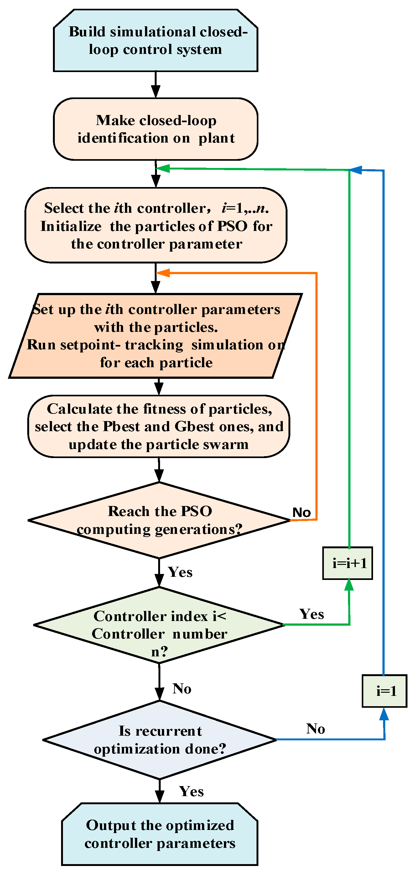
2.4. Iterative-Tuning Monitor

The PSO-RCO method tunes controller parameters in MISO thermal engineering processes through collaborations of each module shown in Figure 1. The overall working flow is organized by the recurrent-optimization monitor and shown in Figure 3. The details of the working flow is explained in the following.

• A closed-loop control simulation model for the thermal engineering process to be optimized should be built first. The utilization of actually applied control algorithm, the sampling data of input variables imported from historical database at big data platform and the accurate dynamic model of the controlled process ensures a high-approximation simulation from the model to the actual process. In the simulation, manipulated variables and controlled variables are produced by the simulation control algorithm and model.
• MISO ARX models for describing the controlled-process dynamics are identified on historical data. The chosen identification data segment includes the samples of manipulated variable, input disturbances and controlled variable. It should keep the identifiable conditions which have been discussed in Section 2.2. By applying the identification algorithms described in Section 2.2.1 and Section 2.2.2, the MISO ARX model of the controlled process can be obtained and imported into the simulation loop. Then an approximate simulation loop of the process is set up.
• The PSO-RCO method optimizes the controllers of a MISO thermal process one by one in several optimization circulations to approach the optimal controller parameters. When the ith (I = 1, 2, n)controller is selected for optimization, the controller parameters like the proportional gain, integral time and derivative gain, are coded into the particles of the PSO algorithm with the initial value of the previous value plusing a random bias. After running the simulation model for enough steps, each particle’s fitness which represents the performance of corresponding controller is evaluated on the fitness function. After enough generations of particle update, the particle swarm converges to the optimal fitness and controller parameters. The optimization result is the new parameters of the ith controller in place of the old ones.
• If the number of controllers in control loop, denoted by n, is larger than 1 and the order of the current optimized controller i is smaller than n, the next controller to be set is the (i + 1)th and let i = i + 1. Then the operations in (3) run again for optimizing the (i + 1)th controller parameters.
• When i reaches n, one round of optimization on multiple controller parameters for the single-output thermal process is done. If the rounds of recurrent parameter-tuning is less than the set number, the next round of optimization is initiated again, starting with the 1st controller and then proceeds to the nth through optimizing process (3). When the rounds of optimization is reached, the whole controller-parameter optimization is finished and the optimized controller parameters are set into the simulation model for verifications. After comparing the optimized control performance with the pre-optimized, the improved controller parameters can be applied to field control system or be a guidance for controller parameter tuning.

3. Verification

The boiler process includes several superheating processes. Each of the processes serve as an energy transferring system, i.e., energy being transferred from the flue gas to the steam. In order to regulate the outlet superheated steam temperature for the sake of safety and high efficiency, each superheater is equipped with desuperheaters which inject desuperheating water at the upstreams of superheater. The desuperheating water is drawn from the boiler feedwater pump.

In Figure 4, the flowchart of a superheater in a 330 MW-rated thermal power unit is shown. The steam flows in two sides of heat-transferring channels in boiler and then merges to be heated by the flue gas in the superheater. In order to keep the outlet superheated steam temperature at setpoint, two desuperheaters are equipped upstream on each side to change the outlet superheated steam temperature. This is a typical MISO control system consisting of two manipulated variables, the positions of A-side and B-side desuperheater valves, and the controlled variable, the outlet superheated steam temperature. Therefore, two desuperheater controllers work in parallel to control two sides of desuperheater valve position, as shown in Figure 5.

In order to optimize the A-side and B-side desuperheater controllers by PSO-RCO, the accurate models of the controlled process should be identified and put into a simulation system in which the control strategy is identical to that in the field. The schematic diagram of the simulation system is shown in Figure 5 where the parameters of the two controllers are adjustable by the result of the PSO-RCO. The PSO-RCO implements the controller optimization through operating the simulation system on field data samples like setpoint, load, inlet steam temperature and other disturbance data, which ensures that the optimization result matches the field controllers. And these field data samples come from the history database on a big data platform which is fed with clean on-line field data after the data preprocess.

3.1. Model Identification

For describing the dynamic characteristics of superheated steam temperature precisely, three models are identified corresponding to three sectors of steam-gas heat exchanging process which are the A-side lead sector, B-side lead sector and the lag sector [19]. Each model is MISO.

Following Principle 1, 8000 continuous samples were picked out of time series, among which the front half was used for identification and the left half for verification. The selected data includes input and output series for the identified MISO models. The three output series are shown as black dash-dot curves in Figure 6, Figure 7 and Figure 8, respectively. The load is varying in this period. Since the variables of a boiler-turbine power-generating process are strongly coupled, the sampled data during this period can meet the condition of persistent excitation on input signals as stated in Principle 1. Checking the time delay and order by cross-correlation function and SVD method, three MISO ARX models were identified by using RLS and then transformed into Z-transfer functions.

The model for A-side lead sector is expressed by

$$\begin{gathered} y_1(z)=G_{1,1}(z)u_{1,1}(z)+G_{1,2}(z)u_{1,2}(z)+G_{1,3}(z)u_{1,3}(z) \\ {G}_{1,1}(z)=\frac{y_1(z)}{u_{1,1}(z)}=\frac{-0.0028z^{-2}}{1+0.9459z^{-1}} \\ {G}_{1,2}(z)=\frac{y_1(z)}{u_{1,2}(z)}=\frac{-0.0187z^{-2}}{1+0.9459z^{-1}} \\ {G}_{1,3}(z)=\frac{y_1(z)}{u_{1,3}(z)}=\frac{-0.0515z^{-2}}{1+0.9459z^{-1}} \end{gathered}$$

(14)

where y₁ denotes the steam temperature at the A-side desuperheater outlet, u_1,1 denotes the power, u_1,2 denotes the opening of A-side desuperheater valve, and u_1,3 denotes the steam temperature at the A-side desuperheater inlet.

The model for B-side lead sector is described by

$$\begin{gathered} y_2(z)=G_{2,1}(z)u_{2,1}(z)+G_{2,2}(z)u_{2,2}(z)+G_{2,3}(z)u_{2,3}(z) \\ {G}_{2,1}(z)=\frac{y_2(z)}{u_{2,1}(z)}=\frac{-0.0070z^{-2}}{1+0.9432z^{-1}} \\ {G}_{2,2}(z)=\frac{y_2(z)}{u_{2,2}(z)}=\frac{-0.0111z^{-2}}{1+0.9432z^{-1}} \\ {G}_{2,3}(z)=\frac{y_2(z)}{u_{2,3}(z)}=\frac{-0.0586z^{-2}}{1+0.9432z^{-1}} \end{gathered}$$

(15)

where y₂ denotes the steam temperature at the B-side desuperheater outlet, u_2,1 denotes the power, u_2,2 denotes the opening of B-side desuperheater valve, and u_2,3 denotes the steam temperature at the B-side desuperheater inlet.

The model for lag sector is described by

$$\begin{gathered} y_3(z)=G_{3,1}(z)u_{3,1}(z)+G_{3,2}(z)u_{3,2}(z)+G_{3,3}(z)u_{3,3}(z) \\ {G}_{3,1}(z)=\frac{z^{-1}(0.0309z^{-1}-0.0042z^{-2}-0.0015z^{-3}-0.0033z^{-4}-0.0074z^{-5}+0.0034z^{-6}-0.0212z^{-7}+0.0007z^{-8})}{1+0.9014z^{-1}+0.1325z^{-2}+0.1207z^{-3}+0.0460z^{-4}-0.0015z^{-5}-0.0501z^{-6}-0.0273z^{-7}-0.1259z^{-8}} \\ {G}_{3,2}(z)=\frac{z^{-1}(0.0269z^{-1}-0.0212z^{-2}+0.0032z^{-3}+0.0026z^{-4}-0.0011z^{-5}-0.0062z^{-6}+0.0089z^{-7}-0.0110z^{-8})}{1+0.9014z^{-1}+0.1325z^{-2}+0.1207z^{-3}+0.0460z^{-4}-0.0015z^{-5}-0.0501z^{-6}-0.0273z^{-7}-0.1259z^{-8}} \\ {G}_{3,3}(z)=\frac{z^{-1}(0.0079z^{-1}+0.0020z^{-2}-0.0111z^{-3}+0.0076z^{-4}-0.0102z^{-5}+0.0039z^{-6}-0.0015z^{-7}+0.0031z^{-8})}{1+0.9014z^{-1}+0.1325z^{-2}+0.1207z^{-3}+0.0460z^{-4}-0.0015z^{-5}-0.0501z^{-6}-0.0273z^{-7}-0.1259z^{-8}} \end{gathered}$$

(16)

where y₃ denotes the superheated steam temperature at the outlet, u_3,1 denotes the steam temperature at the A-side desuperheater outlet, u_3,2 denotes the power, and u_3,3 denotes the steam temperature at the A-side desuperheater outlet. Since the models for A-side and B-side are in series with the model for lag sector, u_3,1 is equal to y₁ and u_3,1 to y₂.

The model-fitting results of three de-mean steam temperatures are shown in Figure 6, Figure 7 and Figure 8. It can be seen that the model outputs are fitting well with the measurement data. The identification models can accurately describe the modelled process in term of dynamics.

3.2. Optimization on Controller Parameters

Based on the complete control system model, the optimization on controller parameters can be initiated after the newly identified parameters set into the plant models. The transfer functions of the A-side and B-side desuperheater controllers are in the following form.

$$W(s)=k_1{k}_p(1+\frac{k_i}{60s})(\frac{60\times k_{d}s+1}{60\times \frac{K_d}{k_a}s+1})$$

(17)

where s is the Laplace operator, k_p is the proportional gain, k_i is the integral gain, k_d is the differential gain, k_a is the filter gain and k₁ is the total gain. The PSO algorithm is taken to optimize k_p, k_i, k_d, k_a for the A-side and B-side desuperheater controllers, k₁ is set as 0.2, and the parameters in objective function (11) and (12) are set as L = 800, w₁ = 3, w₂ = 0.02, w₃ = 0.001, w₄ = 50, w₅ = 60, w₆ = 70.

In the first round of optimization, let β₁ = β₂ = 1 in fitness function (13), and the initial value of the jth particle position vector is generated randomly by

$$x_j(0)=Low+(High-Low)\times rand(0,1),j=1,\cdots ,N$$

(18)

$$Low=[\begin{array}{cccc}{k}_{{}_p}^{-}& k_{{}_i}^{-}& k_{{}_d}^{-}& k_{{}_a}^{-}\end{array}],High=[\begin{array}{cccc}{k}_{{}_p}^{+}& k_{{}_i}^{+}& k_{{}_d}^{+}& k_{{}_a}^{+}\end{array}]$$

(19)

where superscript “+” denotes the high limit of the corresponding variable, and “−” denotes the low limit. From the operating experience of the superheated steam temperature control system, we set $Low=[\begin{array}{cccc}0& 0& 0& 1\end{array}],High=[\begin{array}{cccc}30& 20& 10& 50\end{array}]$. In order to achieve lower optimal controller gain, we set $\begin{array}{ccc}{k}_p^{*}=0.12,& k_i^{*}=0.1,& {\left(k_d/k_a\right)}^{*}=0.12\end{array}$ in objective function (12).

In the succeeding round of optimization, let β₁ = 1, β₂ = 2 in fitness function (13), and the initial value of the jth particle position vector is generated randomly around the optimization result of the previous round, i.e.,

$$x_j(0)=[\begin{array}{cccc}{k}_{{}_p}^0& k_{{}_i}^0& k_{{}_d}^0& k_{{}_a}^0\end{array}]+(rand(0,1)-0.5)[\begin{array}{cccc}{k}_{{}_p}^0& k_{{}_i}^0& k_{{}_d}^0& k_{{}_a}^0\end{array}],j=1,\cdots ,N$$

(20)

where superscript “0” denotes the optimization result of the corresponding variable at the previous round. For a finer adjustment on the acquired controller parameters, we set $\begin{array}{ccc}[k_p^{*},& k_i^{*},& {\left(k_d/k_a\right)}^{*}]\end{array}=[\begin{array}{ccc}{k}_p^0,& k_i^0,& \left(k_{{}_d}^0/k_{{}_a}^0\right)\end{array}]$ in objective function (12).

Fulfilling the working flow in Figure 3 for 5 times and 2 rounds per time, we obtained 5 groups of optimized controller parameters. The optimization results for desuperheater controller A are listed in

Table 1. Optimized controller parameters of desuperheater controller A.

Times	kp	ki	kd	ka
1	10.065	1.436	0.839	15.097
2	10.072	1.456	0.839	15.106
3	10.088	1.444	0.841	15.132
4	10.037	1.480	0.836	15.055
5	10.048	1.457	0.837	15.072
Mean	10.062	1.4546	0.8384	15.0924
Standard deviation	0.02	0.0167	0.0019	0.03

, and controller B in

Table 2. Optimized controller parameters of desuperheater controller B.

Times	kp	ki	kd	ka
1	1.296	2.359	0.108	1.944
2	0.413	5.860	0.034	0.620
3	0.392	6.965	0.033	0.588
4	0.567	5.447	0.047	0.850
5	1.178	2.447	0.098	1.766
Mean	0.7692	4.6156	0.0640	1.1536
Standard deviation	0.4344	2.0949	0.0362	0.6513

.

The tables show that all the optimized gains of controller A and B are in the lower band of their ranges and the optimization results are quite close each time.

Comparing the control results shown in Figure 9, one can find that the root-mean-square error (RMSE) between the controlled variable and setpoint of superheated steam temperature from the optimized control system is much smaller than that from the field original controller, i.e., 1.06 °C vs 2.42 °C. Since the superheated steam channel has many disturbances from steam flow, gas flow and temperature, ash blowing etc., the superheated steam temperature always deviates from its setpoint a lot, resulting in heat efficiency loss or device damage. Figure 9 shows that the optimized controllers can make the RMSE reduced 1.36 °C which will does great benefit to the system operation. Subject to the same range and speed limitations as the original controller outputs, the control variable values from the optimized controller A and B can be seen feasible and reasonable from Figure 10 and Figure 11. Comparing the gains of controller A and B from Table 1 and Table 2, one can find that the proportional gain of controller A is dominated and the integral gain of controller B as well. Therefore, controller A focuses efforts on suppressing deviations of superheated steam temperature from the setpoint during transient process, while controller B focuses on eliminating steady offsets. The optimization result of such a controller function allocation contributes to high-quality control performance in multi-controller-single-output systems. Therefore, the A-side and B-side desuperheater controllers have been effectively optimized by the PSO-RCO parameter-tuning method, and the regulation performance on the superheated steam temperature is greatly improved.

Figure 12 and Figure 13 show the fitness value trends of the global optimal particles in two rounds of PSO optimizations on setting desuperheater controller A and B, respectively. The PSO optimization order in each round is Controller A-Controller B. Each controller parameters are coded by a particle swarm of 30 4-dimensional individuals and experience 20-generation iterative optimization every round. Each of Figure 12 and Figure 13 has two subfigures. The upper one shows the fitness value trend from generation 1–20, and the lower one from generation 21–40. One can observe that there is an obvious drop on the global-best fitness value from generation 20 to generation 21 in Figure 12 or Figure 13. The drop on fitness value of one controller’s particle swarm is caused by the optimization on another controller ahead which improves the overall control performance and reduces the RMSE of the controlled variable. At the beginning of the 2nd round optimization on any one controller, the best fitness value of its particle swarm obviously decreases than it was at the end of the 1st round optimization. Therefore, such recurrently alternative optimizations can greatly speed up the convergence of controller parameters. Since the next round optimization on any one controller always proceeds from a better start point by the optimization on other subsequent controllers in the previous round, the PSO-RCO ensures that the multi-controller parameters in a single process advance in the direction of better system performance.

3.3. Comparisons with Other Methods

The major contribution of this paper is the recurrent multi-objective PSO optimization approach for multiple PID controllers in a single-output system, thus the comparisons to the non-recurrent single-objective PSO optimization as well as recurrent single-objective PSO optimization are made for evaluating the improvement of the proposed method.

(1) Comparison with non-recurrent single-objective optimization

In this non-recurrent single-objective optimization, the multiple-controller parameters are put together to be optimized by the canonical PSO algorithm, and thus the fitness function is given by

$$J={\displaystyle \sum _{j=1}^L(w_1\left|y_j-r_j\right|}+{\displaystyle \sum _{i=1}^{n_u}{w}_{2,i}{u}_{i,j}}+{\displaystyle \sum _{i=1}^{n_u}{w}_{3,i}\left|u_{i,j}-u_{i,j-1}\right|})$$

(21)

where, the number of sampling points L = 800, the number of controllers n_u = 2. Through many trials with different weights of the optimization, it seems that some parameters often reach their limits before convergence, like letting w₁ = 3, w_2,1 = 0.05, w_2,2 = 0.02, w_3,1 = 0.001, w_3,2 = 0.001 and having the optimization result including boundary values listed in

Table 3. Optimized controller parameters of non-recurrent single-objective PSO.

Controller	k1	kp	ki	kd	ka
A	0.2	17.2029	0	7.7268	49.6785
B	0.2	30	20	6.1738	37.3926

. The boundary gains of controller B lead to dramatical movements of desuperheater valve B as shown in Figure 14 and Figure 15 shows that the action of desuperheater valve A is much violent than that from the recurrent multi-objective optimization as shown in Figure 10, due to its higher proportional gain.

(2) Comparison with recurrent single-objective optimization.

The difference between the proposed approach and the recurrent single-objective PSO optimization is that the latter one only use objective function (11) as the fitness function. The parameters in fitness function (11) are set the same as that in multi-objective PSO, i.e., L = 800, w₁ = 3, w₂ = 0.02, w₃ = 0.001, k₁ = 0.2. Through 2 rounds of the working flow in Figure 3 and 15-generation updates for each round, the best one group of optimized controller parameters among several results was obtained and listed in

Table 4. Optimized controller parameters of recurrent single-objective PSO.

Controller	k1	kp	ki	kd	ka
A	0.2	12.6868	1.057	1.9453	12.4708
B	0.2	13.2124	2.1215	2.7846	15.1559

. Comparing with the results from the multi-objective PSO in Table 1 and Table 2, the proportional gains of both sides of controllers are of higher value. Therefore, the controller outputs are more violent as shown in Figure 16 and Figure 17 compared to Figure 10 and Figure 11 resulted from the proposed method. The varying of fitness values of function (11) for the desuperheater controllers A and B are shown in Figure 18 and Figure 19, respectively. In the figures, the circle mark with letter “a” denotes the endpoint of the 1st round of parameter optimization and “b” denotes the startpoint of the 2nd round of optimization for each controller. Figure 19 shows that the fitness value of optimizing desuperheater controller B cannot converge within predetermined 15 generations.

In the recurrent single-objective optimization, as seen from above results, the control parameters converge slowly and the obtained controller gains may be a little higher without involving more objectives like J₂ in optimization. Actually, there are many groups of control parameter combinations in the searching space resulting in acceptable J₁ (possibly not the minimum) in term of practical application. But the higher controller gains represent more energy cost by actuators and more fluctuations in regulating process.

Table 5. Optimized controller parameters of recurrent single-objective PSO.

Methods	Non-Recurrent Single-Objective PSO	Recurrent Single-Objective PSO	Recurrent Multi-Objective PSO
Control RMSE (°C)	1.5964	0.7989	1.06

shows the comparisons among the three methods on RMSE of the controlled variable, i.e., superheated steam temperature. The non-recurrent single-objective PSO achieved the largest RMSE with unreasonable manipulated variable values, the recurrent multi-objective PSO got the moderate result with mild control valve movements, and the recurrent single-objective PSO has the minimal one but with more control energy consumption than the multi-objective PSO. Therefore, the moderate optimization result from the recurrent multi-objective PSO is preferred in practice and the method is better.

4. Discussions

Since the PSO-RCO is based on close-loop simulation, the model accuracy is important for the optimization result. From the field experiment for applying this method, we have some remarks in the following.

Remark 1.

If the identification model is not very precise but can reflect right dynamic trend, the optimized results can be used as a direction-guide for tuning the PID parameters. In this case, it is still very meaningful to process operation because there are multiple parameters in the control system and it is hard to tune the parameters only by trial-and-error.

Remark 2.

If the identification model is accurate enough, like the degree of closed-loop fitting is over 80%, the optimized results can be used in field controllers by little more tuning.

In order to identify more accurate process model for closed-loop simulation, it encourages making full use of big data resources and machine learning approaches [20], e.g., Bayes classifier for filtering sampled data and neural network for nonlinear process identification. Moreover, replacing PID control with advanced approach like model predictive control can greatly improve control performance, and the proposed PSO-RCO method still works for MPC parameter tuning.

The PSO-RCO is not only a controller-parameter recurrent closed-loop tuning method, but also proposes a kind of algorithm framework which is based on the recurrent working flow and involves IC algorithm for multiple-controller-single-output thermal engineering control system optimization. Only canonical PSO was used for optimization in this paper, thus more improvements on PSO-RCO might be achieved if some new methods like fuzzy adaptive PSO, nonlinear time varying PSO and others [21] are introduced into the present algorithm framework.

With the advantage of not interfering system operation, with the potential supporting on big data identification method and with the development of IC algorithms, the PSO-RCO is a promising approach for control system optimization.