Empirical Bayes Prediction in a Sequential Sampling Plan Based on Loss Functions

Abstract

The application of empirical Bayes for lot inspection in sequential sampling plans is usually conducted to estimate the proportion of defective items in the lot rather than for hypothesis testing of the variables’ process mean. In this paper, we propose the use of empirical Bayes in a sequential sampling plan variables’ process mean testing under a squared error loss function and precautionary loss function, for which the prediction is performed to estimate a sequence of the mean when the data are normally distributed in the case of a known mean and unknown variance. The proposed plans are compared with the sequential sampling plan. The proposed techniques yielded smaller average sample number (ASN) and provided higher probability of acceptance (P_a) than the sequential sampling plan.

1. Introduction

Acceptance sampling plans have been widely used in the industry for product quality inspection, with the advantages of destructive testing, large-lot auditing, and ability to choose good history-based suppliers. This method could reduce damage by requiring less product handling, error reduction, and less cost and time restraints in the manufacturing process. Acceptance sampling plans by variables can be classified into two types as follows: Estimation of the percentage of defective units out of the specification limits and statistical hypothesis testing to control the parameters of the process that are measured on a continuous scale, thus providing more information regarding the production in the lots than attributes with a small sample size. The variable sampling plan is utilized as part of quality assurance concerning the average quality of products, such as bulk materials in bags and drums [1], which are one of the variable sampling plan that aims to identify a process mean of the statistical hypothesis testing. Balamurali et al. [2] considered the repetitive group in the variables sampling plan in comparison with single, double, and sequential plans. Sankle and Singh [3] studied the single sampling plan by variables when the data were correlated with a known variance.

The Bayesian approach, as an alternative to the classical approach, is widely used in statistical inferences. Its principle is to incorporate information in the parameters’ history through a prior distribution, assuming a known form of distribution. The parameters of a prior distribution, called hyperparameters, are usually assumed to be known or can be estimated regardless of the observed data. In contrast, when the hyperparameters are unknown and estimated from the observed data, it is called the empirical Bayes (EB) approach [4]. Studies involving EB have been performed by many authors, including Krutchkoff [5], Casella [6], Lu [7], Cui and George [8], Khaledi and Rivaz [9], and Maswadah [10].

The EB approach of estimation parameters can be obtained by using several loss functions, such as the square error loss (SEL) function and precautionary loss (PL) function. The loss functions are considered a loss in the stages of the quality procedure, which reduces the deviation from the true value and increases the target value [11]. They are applied in production quality assurance and the decision-making processes of producers and statisticians. Moskowitz and Tang [12] considered the Bayesian method of estimation parameters using the quadratic loss function and step-loss function applied in a variable acceptance sampling plan in cases of known and unknown variance. Jaheen [13] illustrated EB prediction of the estimation parameter using the linex and quadratic loss function. Naji and Rasheed [14] provided Bayesian estimation based on the PL function, where the parameters were the shape and scale of the Gamma distribution. Research on Bayesian and EB estimation loss functions includes Rahman et al. [15], Zaka and Akhter [16], and Lavanya and Alexander [17].

In addition, EB can be used to estimate newly observed data for predictive purposes, based on the posterior predictive distribution. Gimlin and Breipohl [18] studied the Bayesian approach in a sequential and non-sequential sampling plan of a binomial-distributed random variable with a beta prior distribution and aimed to identify a decision rule with the minimum average risk, using dynamic programming equations. Lam et al. [19] investigated the Bayesian approach in a sequential sampling plan by variables with data normally distributed under an unknown mean and known variance. The Markov technique was used to minimize the expected cost of the optimal sequential sampling plan. Liang et al. [20] studied the efficiency of the Bayesian approach in a sampling plan for lifetime testing under random censoring variables with the exponential distribution using the quadratic loss function in Bayes risk; the proposed plan minimized the total duration of the lifetime. Dunsmore and Wright [21] studied Bayesian prediction in a sequential sampling plan to test the lifetime of items that were taken by a group of items. The random variable followed an exponential distribution with a gamma prior distribution. For the sequential testing at stage k, if a lot was accepted at stage k, with k survivor items, then the predictive distribution was utilized to estimate the average lifetime of the k surviving items.

The EB method was also applied to estimate the percentage of defective units when the lots were accepted [22]. Shin and Shin [23] applied EB for the inspection of a repeated sampling plan by variables and using the data history to estimate the EB estimator, which was based on an estimation of the percentage of defective units. Karunamuni [24] studied EB in a sequential component problem based on an exponential family distribution. The minimum EB risk was used to determine the stopping time in the sequential decision. Delgadillo and Bremer [25] utilized the EB approach, combined with a specified cost function, to test the destruction of high-quality products in a Poisson process. The proposed method was compared with traditional methods, including single, double, multiple, and skip-lot sampling plans.

It can be seen that the sequential sampling plan often provides a smaller average sample number than single, double, or multiple plans. Thus, the sequential sampling plan can be considered as part of destructive testing for high-quality production. In this paper, we propose the use of the EB approach using SEL and PL functions for lot inspection in sequential sampling plans to test variables’ sampling plan process mean. The EB method under the SEL function is easy to calculate, which is the mean of the posterior distribution function and the PL function, and can be applied for reliability and risk analysis. The prediction is then performed to estimate a sequence of the mean under a six-sigma-level quality. The proposed plan is then compared with the traditional approach, the sequential sampling plan by variables. The outline of this paper is as follows. In Section 2, the variable sampling for the process mean testing is described. Next, in Section 3, the traditional plan, sequential sampling plan by variables, is shown. In Section 4, the prediction based on the EB approach under SEL and PL functions is explained. Section 5 and Section 6 cover the results of the simulation and application example. The final section presents the conclusion.

2. Variables Sampling for Process Mean Testing

The variable sampling plan is one of the acceptance sampling plans that is applied in quality assurance of lots. Quality characteristics are measured by a continuous scale [1]. In this paper, the variable process mean is utilized for the statistical hypothesis under a six-sigma quality level, then the process mean has 3.4 defective units per million opportunities $(p)$ and it is assumed to shift to ±1.5$\sigma$. The proportion of defective units in the process is defined by:

$$p=P\left(X>USL|\mu \right)=1-F\left(\frac{USL-\mu }{\sigma }\right),$$

(1)

where USL is an upper specification limit and $F\left(x\right)={\displaystyle {\int }_{-\infty }^x\frac{1}{\sqrt{2\pi }}{e}^{-\frac{z^2}{2}}}dz.$ Thus, the variable process mean hypothesis testing under USL is given by $H_0:{\mu }_2\le {\mu }_1$ vs. $H_1:{\mu }_2>{\mu }_1$, where the parameter ${\mu }_1$ is the acceptable process level (APL) and ${\mu }_2$ is the rejectable process level (RPL). When data are assumed to have a normal distribution: $X\sim N(\mu ,{\sigma }^2)$, where $\sigma$ is known, the parameters ${\mu }_1$ and ${\mu }_2$ can be estimated by:

$$\mathrm{APL}={\mu }_1=P\left(X>USL|{\mu }_1\right)=Mean+1.5{\sigma }_x,$$

and:

$$\mathrm{RPL}={\mu }_2=P\left(X>USL|{\mu }_2\right)=ACL+Z_{\beta }{\sigma }_{\overline{x}},$$

(2)

where $\mathrm{ACL}={\mu }_1+Z_{\alpha }{\sigma }_{\overline{x}}$ are acceptance control limits, $Z\sim N(0,1),$ $\overline{x}$ is the sample mean, ${\sigma }_x$ is the standard deviation of the data, ${\sigma }_{\overline{x}}$ is the standard deviation of the sample mean, the producer’s risk $(\alpha )$ is the probability of rejection at ${\mu }_1$, and the consumer’s risk $(\beta )$ is the probability of acceptance at ${\mu }_2$ [26].

3. Sequential Sampling Plan by Variables

The sequential sampling plan can be categorized by attributes and variables. The sequential sampling plan is modified from the double sampling plan (DSP) and multiple sampling plan (MSP). The samples in this method are taken sequentially, one by one, from the process or lot, called item-by-item sequential sampling. When more than one sample is taken, it is then called group sequential sampling. In addition, the sequential sampling plan by attributes is a one-tailed test because it focuses on an increase of the proportion of the defective when compared with the acceptable quality level (AQL). In contrast, the sequential sampling plan by variables (SSP by variables) can be considered as a one-tailed and two-tailed test: Lower or upper specification limit testing (LSL/USL) and double testing, respectively [1]. Furthermore, when USL is specified, the acceptance limit line (Y₁) and rejection limit line (Y₂) for accepting the lot, continuing sampling, and rejecting the lot are:

$$Y_1=-h_1+s\cdot n\mathrm{and}{Y}_2=h_2+s\cdot n.$$

(3)

Thus, the lot is accepted if ${\displaystyle {\sum }_{i=1}^n{x}_i}\le Y_1$, the lot sampling is continued if $Y_1<{\displaystyle {\sum }_{i=1}^n{x}_i}\text{<}{Y}_2$, and the lot is rejected if ${\displaystyle {\sum }_{i=1}^n{x}_i}\ge Y_2.$ Let $h_1=LB{\sigma }^2/\left({\mu }_2-{\mu }_1\right)$ be the intercept of the acceptance line, $h_2=LA{\sigma }^2/\left({\mu }_2-{\mu }_1\right)$ is the intercept of the rejection line, $s=\left({\mu }_2+{\mu }_1\right)/2$ is the slope of the lines, L is the common logs, and $A=\log \left[\left(1-\beta \right)/\alpha \right]$, $B=\log \left[\left(1-\alpha \right)/\beta \right]$, and known $\sigma$ Generally, the probability of acceptance (P_a) is constructed by:

$$P_a\left(\mu \right)=\left\{{\left[\left(1-\beta \right)/\alpha \right]}^w-1\right\}/{\left[\left(1-\beta \right)/\alpha \right]}^w-{\left[\beta /\left(1-\alpha \right)\right]}^w,$$

(4)

where $w=\left({\mu }_2+{\mu }_1-2\mu \right)/\left({\mu }_2-{\mu }_1\right).$ The average sample number (ASN) [27] is expressed as:

$$ASN\left(\mu \right)=\left[\frac{LA{\sigma }^2}{{\mu }_2-{\mu }_1}+P_a\cdot \left(\frac{L{\sigma }^2\log \left[\beta /\left(1-\alpha \right)\right]-L{\sigma }^{2}A}{{\mu }_2-{\mu }_1}\right)\right]/\left(\frac{2\mu -{\mu }_2-{\mu }_1}{2}\right).$$

(5)

4. Empirical Bayes Prediction Approach

The Bayesian approach is widely applied in statistical inference, where the unknown parameters, $\delta$, are considered as a random variable, depending on information in the history of the parameters, called the prior probability density function, and assuming a known prior distribution, $\pi \left(\delta |\omega \right)$, and known hyperparameter, $\omega .$ Thus, inference concerning $\delta$ is performed using the Bayes’ theorem, which can be expressed up to proportionality as the product of the likelihood function, $L\left(\delta \right)$, and the prior distribution, $\pi \left(\delta |\omega \right).$ The posterior distribution, $h\left(\delta |\underset{\_}{x}\right)$, is obtained as following:

$$h\left(\delta |\underset{\_}{x}\right)=\frac{L\left(\delta \right)\cdot \pi \left(\delta |\omega \right)}{M\left(\underset{\_}{x}|\omega \right)}\propto L\left(\delta \right)\cdot \pi \left(\delta \right),$$

(6)

where $M\left(\underset{\_}{x}|\omega \right)$ denotes the marginal distribution of $\underset{\_}{x}$.

The EB is involved, when the unknown hyperparameter $\left(\omega \right)$ is estimated from the observed data, which do not conform to the Bayesian concept. The hyperparameter can be calculated from the marginal distribution of $\underset{\_}{x}$, given by:

$$M\left(\underset{\_}{x}|\omega \right)={\displaystyle \underset{\delta }{\int }f\left(\underset{\_}{x}|\delta \right)}\cdot \pi \left(\delta |\omega \right)d\delta .$$

(7)

In this case, the observed data, $\underset{\_}{x}$, are a continuous random sample. The predictive distribution function is then developed to estimate the newly observed data or a future observation $(x_{n+1}),$ based on the previous observed data, $x_1,x_2,x_3,...,x_n$ or $\underset{\_}{x},$ which can be derived from:

$$h(x_{n+1}|\underset{\_}{x})={\displaystyle \underset{\delta }{\int }f\left(x_{n+1}|\delta \right)}\cdot h\left(\delta |\underset{\_}{x}\right)d\delta .$$

(8)

Suppose that $f\left(x_{n+1}|\delta \right)$ is a function of the new observed data.

In this paper, we propose the use of EB in the sequential sampling plan (EB in SSP) in the case of a known mean, ${\mu }_0$, and unknown variance, ${\sigma }^2.$ The parameter estimators are determined by SEL and PL functions.

Assuming $X\sim N({\mu }_0,{\sigma }^2),$ informative prior on ${\sigma }^2$: ${\sigma }^2\sim IG(a,b)$, where ${\sigma }^2$ is the parameter and the hyperparameters are $a$ and $b$ that can be estimated from the marginal likelihood distribution as follows.

4.1. Determine the Marginal Likelihood Distribution Function

The hyperparameters $a$ and $b$ are obtained by the marginal likelihood distribution as follows:

$$\begin{array}{ll}M\left(\underset{\_}{x}|a,b\right)& ={\displaystyle \underset{0}{\overset{\infty }{\int }}f\left(\underset{\_}{x}|{\sigma }^2\right)}\cdot \pi \left({\sigma }^2\right)d{\sigma }^2\\ & ={\displaystyle \underset{0}{\overset{\infty }{\int }}\frac{1}{{\left(2\pi {\sigma }^2\right)}^{\raisebox{1ex}{$n$}\!\left/ \!\raisebox{-1ex}{$2$}\right.}}}{e}^{-\frac{1}{2{\sigma }_{}^2}{\displaystyle \sum _{i=1}^n{(x_i-{\mu }_0)}^2}}\cdot \frac{b^a}{\mathsf{\Gamma }\left(a\right)}{\left({\sigma }^2\right)}^{-(a+1)}{e}^{{}^{-\frac{b}{{\sigma }^2}}}d{\sigma }^2\end{array}$$

Then:

$$M\left(\underset{\_}{x}|a,b\right)=\frac{b^a\cdot \mathsf{\Gamma }\left(a+\frac{n}{2}\right)}{{\left(2\pi \right)}^{\raisebox{1ex}{$n$}\!\left/ \!\raisebox{-1ex}{$2$}\right.}\mathsf{\Gamma }\left(a\right){\left[\frac{1}{2}{\displaystyle \sum _{i=1}^n{(x_i-{\mu }_0)}^2}+b\right]}^{\left(a+\frac{n}{2}\right)}}.$$

(9)

Next, if $L(a,b|\underset{\_}{x})=M(\underset{\_}{x}|a,b)$ is not a closed form, the hyperparameters, $a$ and $b$, can be obtained using a numerical method that is utilized by the Newton Raphson method [28]. Then, the estimators, $\widehat{a}$ and $\widehat{b}$, will be substituted into the posterior distribution function.

4.2. Calculate the Posterior Distribution Function of ${\sigma }^2$

The posterior distribution function of ${\sigma }^2$ can be determined as follows:

$$\begin{array}{ll}h\left({\sigma }^2|\underset{\_}{x}\right)& \propto L\left({\sigma }^2|\underset{\_}{x}\right)\pi \left({\sigma }^2\right)\\ & \propto \frac{1}{{\left(2\pi {\sigma }^2\right)}^{\raisebox{1ex}{$n$}\!\left/ \!\raisebox{-1ex}{$2$}\right.}}{e}^{-\frac{1}{2{\sigma }^2}{\displaystyle \sum _{i=1}^n{(x_i-{\mu }_0)}^2}}\cdot \frac{{\widehat{b}}^{\widehat{a}}}{\mathsf{\Gamma }\left(\widehat{a}\right)}{\left({\sigma }^2\right)}^{-(\widehat{a}+1)}{e}^{{}^{-\frac{\widehat{b}}{{\sigma }^2}}}.\end{array}$$

Thus,

$$h\left({\sigma }^2|\underset{\_}{x}\right)\propto {\left({\sigma }^2\right)}^{-\left(\widehat{a}+\frac{n}{2}+1\right)}{e}^{-\frac{1}{{\sigma }^2}\left[\frac{1}{2}{\displaystyle \sum _{i=1}^n{(x_i-{\mu }_0)}^2}+\widehat{b}\right]}.$$

(10)

The posterior distribution function of ${\sigma }^2$ is an inverse gamma distribution, that is:

$${\sigma }^2|\underset{\_}{x}\sim IG\left(\widehat{a}+\frac{n}{2},\widehat{b}+\frac{1}{2}{\displaystyle \sum _{i=1}^n{(x_i-{\mu }_0)}^2}\right).$$

4.3. Obtain the EB Estimator of ${\sigma }^2$ with Respect to the SEL Function

The SEL function format is given by:

$$L\left(t;{\sigma }^2\right)={\left({\sigma }^2-t\right)}^2,$$

(11)

where $t$ is the estimation value of the parameters. Thus, the EB estimator of ${\sigma }^2$ is the mean of the posterior distribution [29], which can be determined by:

$${\widehat{\sigma }}^2{}_{SEL}=E\left({\sigma }^2|\underset{\_}{x}\right).$$

(12)

Thus, the EB estimator of ${\sigma }^2$ under the SEL function is

$${\widehat{\sigma }}^2{}_{SEL}=\frac{\frac{1}{2}{\displaystyle \sum _{i=1}^n{(x_i-{\mu }_0)}^2}+\widehat{b}}{\widehat{a}+\frac{n}{2}-2}.$$

(13)

4.4. Determine the EB Estimator of ${\sigma }^2$ with Respect to the PL Function

The PL function format is provided by:

$$L\left(t;{\sigma }^2\right)=\frac{{\left({\sigma }^2-t\right)}^2}{t}.$$

(14)

The EB estimator of ${\sigma }^2$ for PL [29] is determined by:

$${\widehat{\sigma }}_{PL}^2=\sqrt{E\left[{\left({\sigma }^2\right)}^2|\underset{\_}{x}\right]}.$$

(15)

Then, the estimator under PL can be obtained [30] as follows:

$$\begin{array}{ll}E\left[{\left({\sigma }^2\right)}^2|\underset{\_}{x}\right]& ={\displaystyle \underset{0}{\overset{\infty }{\int }}{\left({\sigma }^2\right)}^2\cdot h\left({\sigma }^2|\underset{\_}{x}\right)}d{\sigma }^2\\ & ={\displaystyle \underset{0}{\overset{\infty }{\int }}{\left({\sigma }^2\right)}^2\cdot {\left({\sigma }^2\right)}^{-\left(\widehat{a}+\frac{n}{2}+1\right)}{e}^{-\frac{1}{{\sigma }^2}\left[\frac{1}{2}{\displaystyle \sum _{i=1}^n{(x_i-{\mu }_0)}^2}+\widehat{b}\right]}}d{\sigma }^2.\end{array}$$

(16)

From Equation (16), the estimator of ${\sigma }^2$ under PL is:

$${\widehat{\sigma }}_{PL}^2=\sqrt{\frac{{\left[\frac{1}{2}{\displaystyle \sum _{i=1}^n{(x_i-{\mu }_0)}^2}+\widehat{b}\right]}^{\left(\widehat{a}+\frac{n}{2}-2\right)}}{\mathsf{\Gamma }\left(\widehat{a}+\frac{n}{2}-2\right)}}.$$

After that, the estimators of ${\widehat{\sigma }}^2{}_{SEL}$ and ${\widehat{\sigma }}^2{}_{PL}$ will be replaced into the posterior predictive distribution function.

4.5. Construct the Posterior Predictive Distribution Function of $x_{n+1}|\underset{\_}{x}$

The posterior predictive distribution function can be calculated as follows:

$$\begin{array}{ll}h\left(x_{n+1}|\underset{\_}{x}\right)& ={\displaystyle \underset{0}{\overset{\infty }{\int }}f\left(x_{n+1}|{\sigma }^2\right)}\cdot h\left({\sigma }^2|\underset{\_}{x}\right)d{\sigma }^2\\ & ={\displaystyle \underset{0}{\overset{\infty }{\int }}\frac{1}{\sqrt{2\pi {\sigma }^2}}}{e}^{-\frac{1}{2{\sigma }_{}^2}{(x_{n+1}-{\mu }_0)}^2}{\frac{\left[\widehat{b}+\frac{1}{2}{\displaystyle \sum _{i=1}^n{(x_i-{\mu }_0)}^2}\right]}{\mathsf{\Gamma }\left(\widehat{a}+\frac{n}{2}\right)}}^{\left(\widehat{a}+\frac{n}{2}\right)}\\ & \times {\left({\sigma }^2\right)}^{-(\widehat{a}+\frac{n}{2}+1)}{e}^{-\frac{1}{{\sigma }^2}\left[\widehat{b}+\frac{1}{2}{\displaystyle \sum _{i=1}^n{(x_i-{\mu }_0)}^2}\right]}d{\sigma }^2.\end{array}$$

Thus,

$$\begin{array}{ll}h\left(x_{n+1}|\underset{\_}{x}\right)=& \frac{\mathsf{\Gamma }\left(\frac{2\widehat{a}+n+1}{2}\right)}{\mathsf{\Gamma }\left(\frac{2\widehat{a}+n}{2}\right){\left\{\pi \cdot \left(2\widehat{a}+n\right)\left(\frac{2}{2\widehat{a}+n}\right)\left[\widehat{b}+\frac{1}{2}{\displaystyle \sum _{i=1}^n{(x_i-{\mu }_0)}^2}\right]\right\}}^{\frac{1}{2}}}\\ & \times {\left\{1+\frac{1}{\left(2\widehat{a}+n\right)}\frac{{(x_{n+1}-{\mu }_0)}^2}{\left(\frac{2}{2\widehat{a}+n}\right)\left[\widehat{b}+\frac{1}{2}{\displaystyle \sum _{i=1}^n{(x_i-{\mu }_0)}^2}\right]}\right\}}^{-\left(\frac{2\widehat{a}+n+1}{2}\right)}.\end{array}$$

(17)

The results show that the posterior predictive distribution function, $x_{n+1}|\underset{\_}{x}$, is a location-scale t-distribution, that is:

$$x_{n+1}|\underset{\_}{x}\sim t\left(\nu ,{\mu }_0,\lambda \right),$$

where:

$$\nu =2\widehat{a}+n,$$

and:

$$\lambda =\left(\frac{2}{2\widehat{a}+n}\right)\left[\widehat{b}+\frac{1}{2}{\displaystyle \sum _{i=1}^n{(x_i-{\mu }_0)}^2}\right].$$

5. Numerical and Results

In this study, we considered the variables process mean hypothesis USL testing under $H_0:{\mu }_2\le {\mu }_1$ vs. $H_1:{\mu }_2>{\mu }_1$, where there is a comparison of two methods according to the SSP by variables and EB in SSP. In the case of EB in SSP, we considered the case of a known mean, $\mu$, and unknown variance, ${\sigma }^2,$ assuming informative prior on ${\sigma }^2$:${\sigma }^2\sim IG(a,b),$ where $a$ and $b$ denote hyperparameters. The parameter ${\sigma }^2$ is determined from SEL and PL functions. The hyperparameters, $a$ and $b$, are obtained by Newton-Raphson. The data are generated from a standard normal distribution, the lot size is specified by $N$ = 1000, the sample size is defined by $n$ = 50, and the number of iterations is given by $t$ = 1000. The proportion of defective units is determined by a six-sigma process level in which the proportion of defective units at APL is $p$ = 0.00034, $\alpha$ = 0.05, and $\beta$ = 0.10. The P_a and the ASN are considered as the criteria for comparison. The result of the simulation with the two approaches is expressed in

Table 1. Comparison P_a and ASN of SSP by variables, EB in SSP for SEL and PL.

Pa			ASN
SSP	EB in SSP (SEL)	EB in SSP (PL)	SSP	EB in SSP (SEL)	EB in SSP (PL)
0.9662	0.9990	0.9977	21.1673	10.9694	12.4706
0.9598	0.9796	0.9998 *	22.0605	18.8427	5.4135
0.9548	0.9976	0.9993 *	22.7102	12.5077	10.5291
0.8883	0.9997	0.9980	28.5539	5.1358	3.4486
0.9568	0.9999 *	0.9990	22.4496	8.5023	4.9671
0.9448	0.9996	0.9987 *	23.8553	9.9511	8.4201
0.9645	0.1617	0.9599	21.4148	38.1324	22.0460
0.9703	0.9993	0.9989 *	20.5323	10.3801	6.6090
0.9235	0.9999 *	0.9995 *	25.9091	4.7902	3.9721
0.9642	0.9963	0.9994 *	21.4582	13.4647	9.9028
0.9407	0.8658	0.9762	24.2880	29.9258	19.5063
0.9651	0.9941	0.9995 *	21.3328	14.6292	9.9395
0.9767	0.2157	0.9288	19.4190	33.5929	34.0495
0.8998	0.9998 *	0.9987 *	27.7680	8.7000	11.3738
0.9521	0.9997 *	0.9997 *	23.0272	4.1074	4.8513
0.9735	0.9996	0.9996 *	19.9923	9.6105	6.4155
0.9586	0.9997 *	0.9998 *	22.2191	7.2359	6.0929
0.9691	0.9999 *	0.9315	20.7170	8.0689	25.1862
0.9437	0.9785	0.9882	23.9723	15.8336	2.7129
0.9577	0.9775	0.9243	22.3429	19.2633	25.8429
0.9434	0.9998 *	0.9991	24.0095	9.0979	7.4710
0.9544	0.9999 *	0.9996 *	22.7502	7.7668	7.5423
0.9586	0.9998 *	0.9994 *	22.2226	4.9286	5.1259
0.8849	0.9999 *	0.9998 *	28.7711	8.2136	6.7508
0.9463	0.9901	0.9990 *	23.6941	6.5899	7.0308
0.9482	0.9932	0.9998 *	23.4808	15.0636	8.8335
0.9386	0.9970	0.9994 *	24.5044	12.9948	10.1527
0.9154	0.9998 *	0.9993 *	26.5839	8.9655	7.8158
0.9444	0.9904	0.9989 *	23.8986	6.2963	6.8308
0.9748	0.9986	0.9999 *	19.7757	11.5157	8.1897
0.9748	0.8417	0.9999 *	21.7248	31.3442	15.1279
0.9623	0.9748	0.9930	25.2059	19.7683	17.1843
0.9313	0.9954	0.9867	21.5153	6.1856	6.4932
0.9638	0.9999 *	0.9980	23.5936	8.3319	5.9042
0.9472	0.9999 *	0.9974	25.5931	4.6231	5.1422
0.9271	0.9998 *	0.9996 *	21.5357	7.0424	6.6292
0.9637	0.8614	0.9894	26.0231	31.2110	9.7624
0.9222	0.9997 *	0.9996 *	23.5789	9.2951	6.9346
0.9463	0.9901	0.9997 *	23.6941	6.5899	7.0308
0.9473	0.9999 *	0.9983	23.2380	7.8688	11.2152
0.9503	0.9985	0.9988	22.7621	6.8328	7.9634
0.9543	0.9995	0.9999 *	26.4014	10.1902	9.3346
0.9177	0.9999 *	0.9997 *	21.9923	8.2467	7.6790
0.9604	0.9999 *	0.9999 *	22.6079	8.3337	6.3901
0.9556	0.9967	0.9931	20.8212	6.0245	6.3629
0.9685	0.9997 *	0.9935	23.2112	4.3715	4.7472
0.9506	0.9994 *	0.9990	22.7027	10.3105	5.9873
0.9548	0.9999 *	0.9969	22.9562	7.7538	7.1945
0.9527	0.9994 *	0.9974	22.8379	10.2288	8.6005
0.9537	0.9968	0.9853	22.9239	6.0038	5.7879
0.9530	0.9690	0.9998 *	27.7936	20.7371	9.7188
-	0.9998 *	0.9959	-	6.9083	6.9956

* is the estimated value difference at the fifth decimals position.

.

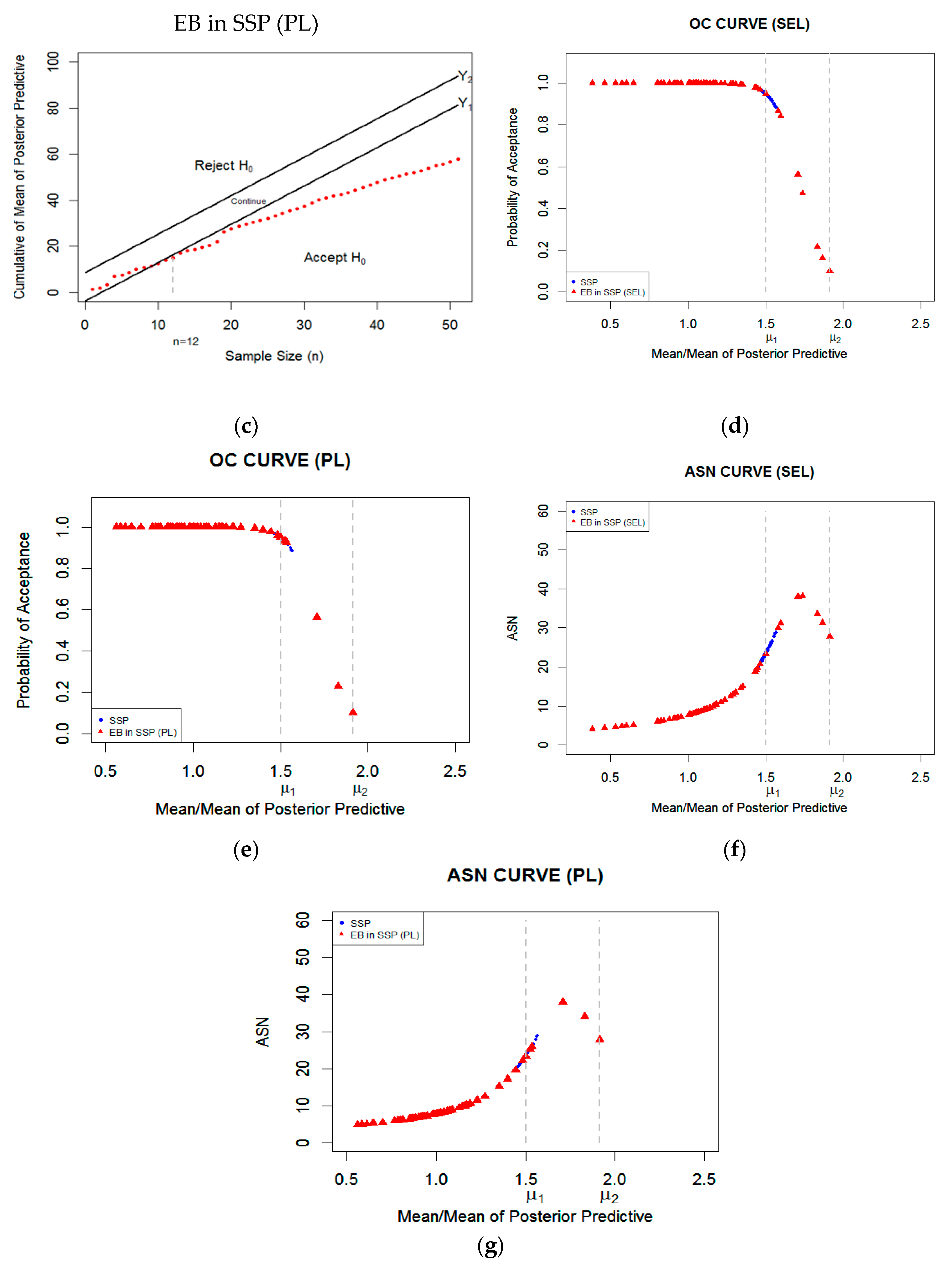
In this paper, we considered the process mean USL testing with SSP by variables and EB in SSP using SEL and PL functions. When ${\mu }_1$ and ${\mu }_2$ were determined by referring to Equation (2) and then ${\mu }_1$ = 1.50 and ${\mu }_2$ = 1.92. In addition, Figure 1a–c show that when the process mean USL testing with SSP by variables and EB in SSP using SEL and PL functions, the limit lines for SSP by variables and EB in SSP approaches are included as follows: The acceptance limit line (Y₁) and rejection limit line (Y₂), where $h_1$ = 5.4387 and $h_2$ = 6.9826. It can be seen that the results of SSP by variable testing found that the cumulative of the sample mean are compared with $Y_1$ and $Y_2$, then the cumulative of sample mean are less than $Y_1$ at the sample size n = 26. That is, to accept $H_0$, and then the lot is accepted. Next, the EB in SSP for SEL and PL under USL testing are considered, where $Y_1,$ $Y_2,$ $h_1$ = 5.4387 and $h_2$ = 6.9826 are considered similar to the case of the SSP by variables. The hyperparameter estimators, $\widehat{a}$ and $\widehat{b}$, are obtained from the Newton-Raphson numerical. The results of the EB in SSP for SEL and PL cases provide that the cumulative of the mean of the posterior predictive distribution $\left(E(x_{n+1}|\underset{\_}{x})\right)$ are comparable with $Y_1$ and $Y_2$, indicating that the $E(x_{n+1}|\underset{\_}{x})$ is less than $Y_1$, the result of which is to accept $H_0$ or the lot is accepted at the sample size n = 9 and n = 12. Thus, the proposed plans provide smaller sample sizes than SSP by variables.

In addition, the process mean USL testing with SSP by variables and EB in SSP using SEL and PL functions can be considered by P_a and ASN. Table 1 shows that the P_a and ASN of EB in SSP for SEL and PL are comparable with SSP by variables. The P_a can be calculated by using Equation (4). The P_a of the SSP by variables is the smallest, which is around 0.8849 to 0.9767, and it has a decreasing trend when the averages are large. However, the majority of the P_a for EB in SSP for SEL and PL yield the highest P_a that is stable close to 0.99. It is evident that P_a of the proposed plans provides a higher and wider spread than the SSP by the variables, as can be seen in Figure 1d,e, respectively.

Furthermore, the ASN for SSP by variables and EB in SSP can be calculated from Equation (5), for which the values of ASN for the SSP by variables are between 19 and 29 per lot. The majority of the ASN for the EB in SSP for SEL and PL are the smallest, from 4 to 25 per lot. Thus, it can be seen that the ASN values of the proposed plans are smaller and more spread than the SSP by variables. It can be seen in Figure 1f,g, respectively.

6. An Application Example

Real data considers liquid crystals’ display with super twisted nematic (STN) technology for improvement of the LCD, which is considered the thickness of the liquid crystals’ display [31]. APL(${\mu }_1$) is 0.70 mm, RPL(${\mu }_2$) is 0.77 mm, $\alpha$= 0.05, and $\beta$= 0.10. This data are observed by n = 79 as follows:

0.717, 0.698, 0.726, 0.684, 0.727, 0.688, 0.708, 0.703, 0.694, 0.713, 0.730, 0.699, 0.710, 0.688, 0.665, 0.704, 0.725, 0.729, 0.716, 0.685, 0.712, 0.716, 0.712, 0.733, 0.709, 0.703, 0.730, 0.716, 0.688, 0.688, 0.712, 0.702, 0.726, 0.669, 0.718, 0.714, 0.726, 0.683, 0.713, 0.737, 0.740, 0.706, 0.726, 0.688, 0.715, 0.704, 0.724, 0.713, 0.694, 0.742, 0.690, 0.704, 0.697, 0.705, 0.707, 0.687, 0.718, 0.718, 0.724, 0.706, 0.687, 0.673, 0.730, 0.732, 0.720, 0.688, 0.710, 0.707, 0.706, 0.709, 0.729, 0.729, 0.685, 0.686, 0.722, 0.720, 0.715, 0.727, 0.696.

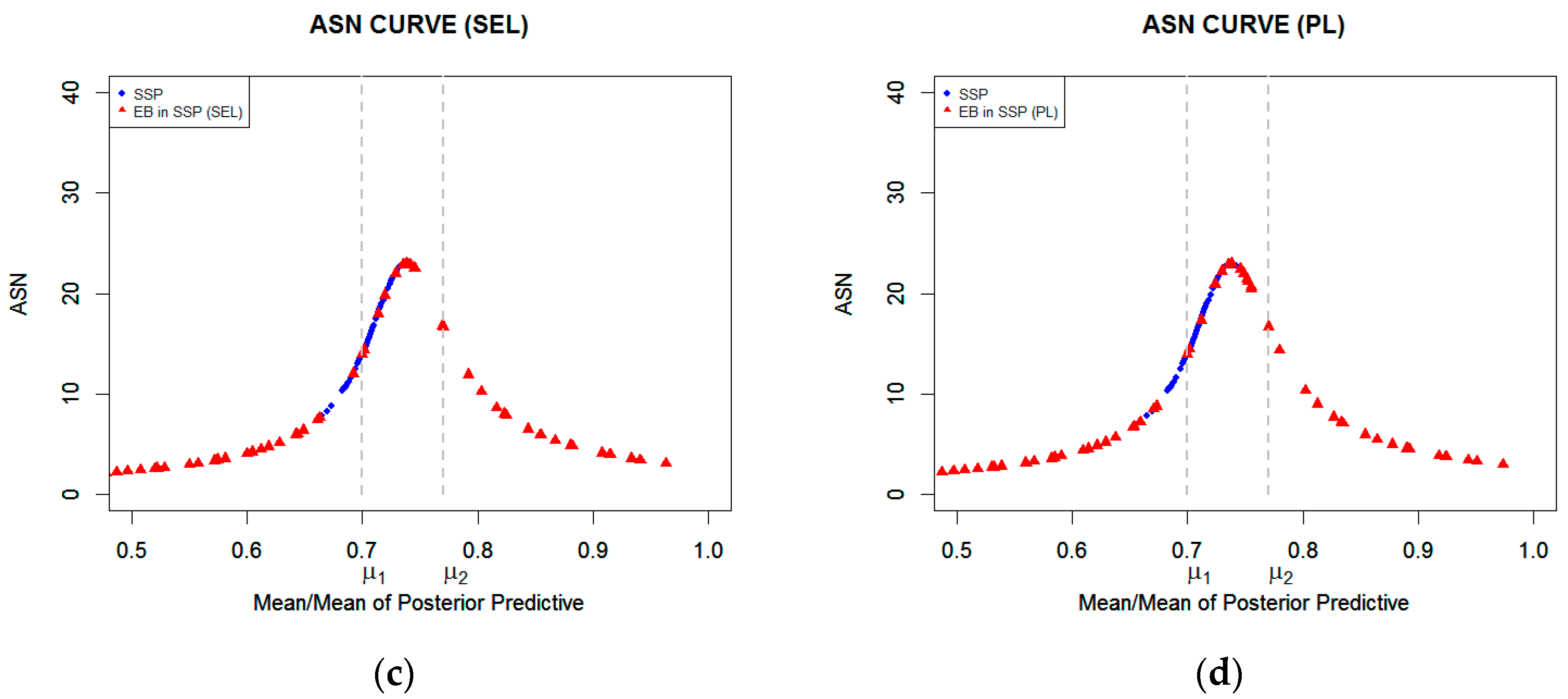
The sample mean of this data is 0.7088 and the standard deviation is 0.0172. The results show that the majority of the P_a values of EB in SSP for SEL and PL provide higher values than SSP by variables, which is about 0.99, as can be seen in Figure 2a,b, respectively. In contrast, the ASN of the two proposed plans is mostly smaller than the SSP by variables, which are provided in Figure 2c,d. Therefore, it is clear that the result of EB in SSP for SEL and PL in the data provide similar simulation results.

7. Conclusions

In this paper, we considered the EB in SSP using SEL and PL functions for variables’ process mean USL testing when data were assumed to be normally distributed under a situation of a known mean and unknown variance. The lot size was $N$ = 1000, the sample size was $n$ = 50, and the number of iterations was $t$ = 1000. The proportion of defective units was determined by a six-sigma process level in which the proportion of defective units at APL was $p$ = 0.00034, $\alpha$ = 0.05, and $\beta$ = 0.10. The proposed plans were compared with the traditional SSP by variables. The result indicated that the proposed methods provides a higher P_a and smaller ASN than the traditional approach. The proposed methods also provided promising results in a real situation for variables’ process mean testing and reduced the producer’s risk, including cost savings in inspecting products in the lot. It is clear that the EB in SSP under SEL and PL functions use the data twice because of the prior distribution having less knowledge about the parameters. Thus, it is a good technique for solving this problem, which is to estimate the hyperparameters from observed data. It can be seen that the proposed plans are more sufficient than SSP by variables because they can reduce the sample size or ASN for inspection of the lot and provide high values of P_a. In addition, we applied the proposed plan to real data of a liquid crystal display with super twisted nematic (STN) technology for improvement of the LCD, which yielded consistent results with those in the simulation. In future research, the EB in the SSP approach can be compared with other plans. The EB in the SSP approach can be performed using different types of priors and data.

References

1. Montgomery, D.C. Statistical Quality Control: A Modern Introduction, 6th ed.; Jonh Wiley & Sons: New York, NY, USA, 2009. [Google Scholar]
2. Balamurali, S.; Park, H.; Jun, C.-H.; Kim, K.-J.; Lee, J. Designing of Variables Repetitive Group Sampling Plan Involving Minimum Average Sample Number. Commun. Stat.-Simul. Comput. 2005, 34, 799–809. [Google Scholar] [CrossRef]
3. Sankle, R.; Singh, J.R. Single Sampling Plans for Variables Indexed by AQL and AOQL with Measurement Error. J. Mod. Appl. Stat. Methods 2012, 11, 396–406. [Google Scholar] [CrossRef] [Green Version]
4. Carlin, B.P.; Louis, T.A. Bayesian Methods for Data Analysis, 3rd ed.; Chapman & Hall/CRC: Boca Raton, FL, USA, 2009. [Google Scholar]
5. Krutchkoff, R.G. Empirical Bayes Estimation. Am. Stat. Assoc. 1972, 26, 14–16. [Google Scholar]
6. Casella, G. An Introduction to Empirical Bayes Data Analysis. Am. Stat. Assoc. 1985, 39, 83–87. [Google Scholar]
7. Lu, W.-S. The efficiency of the method of moments estimates for hyperparameters in the empirical Bayes binomial model. Comput. Stat. 1999, 14, 263–276. [Google Scholar] [CrossRef]
8. Cui, W.; George, E.I. Empirical Bayes vs. fully Bayes variable selection. J. Stat. Plan. Inference 2008, 138, 888–900. [Google Scholar] [CrossRef]
9. Khaledi, M.J.; Rivaz, F. Empirical Bayes spatial prediction using a Monte Carlo EM algorithm. Stat. Methods Appl. 2009, 18, 35–47. [Google Scholar] [CrossRef]
10. Maswadah, M. Empirical Bayes inference for the Weibull model. Comput. Stat. 2013, 28, 2849–2859. [Google Scholar] [CrossRef]
11. Spiring, F.A. The Reflected Normal Loss Function. Can. J. Stat. 1993, 21, 321–330. [Google Scholar] [CrossRef]
12. Moskowitz, H.; Tang, K. Bayesian Variables Acceptance-Sampling Plans: Quadratic Loss Function and Step-Loss Function. Technometrics 1992, 34, 340–347. [Google Scholar] [CrossRef]
13. Jaheen, Z.F. Empirical Bayes analysis of record statistics based on linex and quadratic loss functions. Comput. Math. Appl. 2004, 47, 947–954. [Google Scholar] [CrossRef] [Green Version]
14. Naji, L.F.; Rasheed, H.A. Bayesian Estimation for Two Parameters of Gamma Distribution under Precautionary Loss Function. Ibn AL-Haitham J. Pure Appl. Sci. 2019, 32, 187–196. [Google Scholar] [CrossRef]
15. Rahman, H.; Roy, M.K.; Baizid, A. Bayes Estimation under Conjugate Prior for the Case of Power Function Distribution. Am. J. Math. Stat. 2012, 2, 44–48. [Google Scholar] [CrossRef]
16. Zaka, A.; Akhter, A.S. Bayesian Analysis of Power Function Distribution Using Different Loss Functions. Int. J. Hybrid Inf. Technol. 2014, 7, 229–244. [Google Scholar] [CrossRef]
17. Lavanya, A.; Alexander, T.L. Estimation of Parameters Using Lindley’s Method. Int. J. Adv. Res. 2016, 4, 1767–1778. [Google Scholar] [CrossRef] [Green Version]
18. Gimlin, D.R.; Breipohl, A.M. Bayesian Acceptance Sampling. IEEE Trans. Reliab. 1972, R-21, 176–180. [Google Scholar] [CrossRef]
19. Lam, Y.; Li, K.H.; Ip, W.-C.; Wong, H. Sequential variable sampling plan for normal distribution. Eur. J. Oper. Res. 2006, 172, 127–145. [Google Scholar] [CrossRef]
20. Liang, T.; Chen, L.-S.; Yang, M.-C. Efficient Bayesian sampling plans for exponential distributions with random censoring. J. Stat. Plan. Inference 2012, 142, 537–551. [Google Scholar] [CrossRef]
21. Dunsmore, I.R.; Wright, D.E. A Decisive Predictive Approach to the Construction of Sequential Acceptance Sampling Plans for Lifetimes. J. R. Stat. Soc. Ser. C 1985, 34, 1–13. [Google Scholar] [CrossRef]
22. Ohta, H.; Ogawa, S. Design of Economic Sampling Plan Based on Empirical Bayesian Approach. Front. Stat. Qual. Control 4 1992, 4, 100–108. [Google Scholar]
23. Shin, M.-W.; Shin, K.I. Empirical Bayes Estimation on Sampling Inspection by Variables. J. Korean Soc. Qual. Manag. 1995, 23, 45. [Google Scholar]
24. Karunamuni, R.J. Empirical Bayes Sequential Estimation for Exponential Family: The Untruncated Component. Ann. Inst. Stat. Math. 1996, 48, 711–730. [Google Scholar] [CrossRef]
25. Delgadillo, F.; Bremer, R. The development of a destructive sampling method designed for high quality production processes (DSM-HQ). Qual. Quant. 2010, 44, 595–605. [Google Scholar] [CrossRef]
26. Taherian, T.; Asl, M.B. Capability Analysis and use of Acceptance and Control Charts in the 6-Sigma in Pharmaceutical Industries Case Study: Behestan Tolid Pharmaceutical Co. Int. J. Appl. Inf. Syst. 2016, 11, 127–135. [Google Scholar]
27. Schilling, E.G.; Neubauer, D.V. Acceptance Sampling in Quality Control, 2nd ed.; Chapman & Hall/CRC: Boca Raton, FL, USA, 2009. [Google Scholar]
28. Garthwaite, P.; Jolliffe, I.; Jones, B. Statistical Inference, 2nd ed.; Oxford University Press: New York, NY, USA, 2002. [Google Scholar]
29. Ali, S.; Aslam, M.; Kazmi, S.M.A. A Study of the Effect of the loss function on Bayes Estimate, posterior risk and hazard function for Lindley distribution. Appl. Math. Model. 2013, 37, 6068–6078. [Google Scholar] [CrossRef]
30. Rasheed, A.H.; Raghda, A. Reliability Estimation in Inverse Rayleigh Distribution Using Precautionary Loss Function. Math. Stat. J. 2016, 2, 9–15. [Google Scholar]
31. Wu, C.-W.; Pearn, W.L. A variables sampling plan based on Cpmk for product acceptance determination. Eur. J. Oper. Res. 2008, 184, 549–560. [Google Scholar] [CrossRef]
Figure 1. (a) The cumulative of sample mean with the sequential sampling plan (SSP) by variables versus sample size (n); (b) The cumulative of E ( x n + 1 | x _ ) with empirical Bayes in sequential sampling plan (EB in SSP) for square error loss (SEL) function at various sample sizes; (c) The cumulative of E ( x n + 1 | x _ ) with EB in SSP for precautionary loss (PL) function at various sample sizes (d) The comparison Pa of SSP by variables and EB in SSP for SEL; (e) The comparison Pa of SSP by variables and EB in SSP for PL; (f) The comparison ASN of the SSP by variables and EB in SSP for SEL; (g) The comparison ASN of the SSP by variables and EB in SSP for PL.
Processes 07 00944 g001aProcesses 07 00944 g001b
Figure 2. (a) The comparison Pa of SSP by variables and EB in SSP for SEL in real data; (b) The comparison Pa of SSP by variables and EB in SSP for PL in real data; (c) The comparison ASN of the SSP by variables and EB in SSP for SEL in real data; (d) The comparison ASN of the SSP by variables and EB in SSP for PL in real data.
Processes 07 00944 g002aProcesses 07 00944 g002b