Abstract
Energy is one of the valuable resources in this biosphere. However, with the rapid increase of the population and increasing dependency on the daily use of energy due to smart technologies and the Internet of Things (IoT), the existing resources are becoming scarce. Therefore, to have an optimum usage of the existing energy resources on the consumer side, new techniques and algorithms are being discovered and used in the energy optimization process in the smart grid (SG). In SG, because of the possibility of bi-directional power flow and communication between the utility and consumers, an active and optimized energy scheduling technique is essential, which minimizes the end-user electricity bill, reduces the peak-to-average power ratio (PAR) and reduces the frequency of interruptions. Because of the varying nature of the power consumption patterns of consumers, optimized scheduling of energy consumption is a challenging task. For the maximum benefit of both the utility and consumers, to decide whether to store, buy or sale extra energy, such active environmental features must also be taken into consideration. This paper presents two bio-inspired energy optimization techniques; the grasshopper optimization algorithm (GOA) and bacterial foraging algorithm (BFA), for power scheduling in a single office. It is clear from the simulation results that the consumer electricity bill can be reduced by more than 34.69% and 37.47%, while PAR has a reduction of 56.20% and 20.87% with GOA and BFA scheduling, respectively, as compared to unscheduled energy consumption with the day-ahead pricing (DAP) scheme.
1. Introduction
With the increased use of modern technologies and smart appliances in every field of life, energy consumption is rapidly increasing. The rising electricity demand cannot be fulfilled by the traditional electric power grid. That is why the smart grid is becoming more popular to fulfil daily electricity demand. The smart grid (SG) is supposed to be the incorporation of information technologies (IT) in the existing power grids to increase their robustness and consistency. Smart meters (SM) are used for communication and energy monitoring purposes in SG. To schedule smart appliances in residential, commercial and industrial sectors, an energy management controller (EMC) is installed at the consumer premises. Demand side management (DSM) has many strategies that help to solve the energy optimization problem by peak clipping, load shifting, strategic conservation, flexible load shifting, strategic load growth and valley filling. By using these strategies, the load is shifted from high demand timings to low demand timings [1]. The two main functionalities of DSM are proper management of the load and demand response (DR) [2]. Consumer load management is also known as DSM. It is the process of shifting electricity demand from high-demand (on-peak) hours to low-demand(off-peak) hours to decrease the energy cost. DR is the consumer’s response to variable pricing signals. There are two shapes of DR: in the form of energy price reduction or some incentives to consumers [3,4].
The main objectives of the energy management system (EMS) are the reduction of the energy bill, PAR and consumer discomfort. Many algorithms have been deigned to accomplish the aforementioned objectives. For cost and energy consumption minimization, mixed integer linear programming (MILP), mixed integer nonlinear programming (MINLP), non-integer linear programming (NILP) and convex programming were used in [5,6,7,8]. However, these techniques are used for fewer appliances and have a large convergence time. In order to overcome these deficiencies, researchers use meta-heuristic techniques to resolve the issue of energy optimization. For cost minimization, the genetic algorithm (GA) was proposed by the authors in [9,10]. For cost minimization and aggregated power consumption, differential evolution (DE) and ant colony optimization (ACO) were used in [11,12].
In this research work, we use GOA and BFA techniques for a single office using the DAP pricing signal. The simulation is performed in MATLAB, and we obtained the results of PAR, cost and average waiting time. The rest of the paper is divided into the following sections: Related work is illustrated in Section 2. Section 3 discusses the problem statement and approach. Section 4 depicts the system model and problem formulation. The proposed schemes are described in Section 5. Simulation results are illustrated in Section 6 to demonstrate some of the achievements. The paper is concluded in Section 7.
2. Related Work
In SG, numerous algorithms have been proposed by researches, for energy-efficient optimization in residential, commercial and industrial areas, for the benefits of both consumers and the utility. The main targets of researchers have been balancing the load and decreasing electricity cost. Different parameters such as pricing mechanisms, types of appliances and different user demands are considered.
Hybrid bacterial foraging and genetic (HBG) algorithm-based DSM for smart homes was proposed by the authors in [13]. They focused on peak load reduction, cost minimization, user comfort maximization and load shifting. Through HBG cost, PAR and waiting time were reduced compared to GA and BFA. A smart community-based energy optimization technique was discussed in [14]. The authors focused on the end-user’s high comfort level and less energy usage with integration of renewable energy sources using particle swarm optimization (PSO). A time-constrained nature-inspired algorithm-based home energy management (HEM) system was proposed by the authors in [15]. GA, moth-flame optimization algorithm (MFO) and their hybridization were proposed for energy bill reduction and achieving end-users’ high comfort level. A HEM system using cuckoo search was proposed in [16]. The performance of GA and the cuckoo search algorithm was compared with respect to the reduction of energy cost, PAR and user discomfort by using the DAP signal. Cuckoo search incorporation with levy flights of some kind of birds and fruit-flies were considered for the breading strategy in [17]. In many optimization problems, because of its generic and robust nature, the cuckoo search is superior to GA and PSO. The authors used GA, TLBO (teacher learning-based algorithm), LP (linear programming) and TLGO (teacher learning genetic optimization) algorithms for appliances scheduling in [18]. They categorized flexible appliances as “time flexible” and “power flexible” for proficient energy consumption of consumers in SG. This approach enables energy consumers to schedule their appliances to get optimized energy consumption. This approach also maximizes the comfort level of customers with restricted total energy consumption. In [19], the authors discussed optimal operation methods for a micro-grid. They used the improved adaptive evolutionary algorithm and swarm optimization algorithm. In [20], the authors presented an optimal scheduling scheme for residential appliances, using the DAP signal in smart homes. This algorithm reduced peak cost to 22.6% and normal price to 11.7%. This approach does not rely on the energy optimization approach. In [21], the authors discussed load shifting, cost minimization and the energy storage system (ESS). They proposed a system that enables the user to buy energy during low demand timings and sale their stored energy to the utility during on-peak hours.
In [22], the gradient-based particle swarm optimization (GPSO) technique for demand response (DR) in smart homes, considering the load and energy price uncertainties, was discussed. Having an optimal scheduling of power, the heuristic-based genetic algorithm (GA) was used for demand response (DR) in HEM systems in [23]. In this paper, the authors used GA, TLBO (teaching learning-based optimization), EDE (enhanced differential evolution) and proposed EDTLA (enhanced differential teaching learning algorithm) for minimization of the residential total energy cost and end-user discomfort level. The authors in [24] discussed the cooperative multi-swarm particle swarm optimization (PSO) technique for achieving their goals of cost minimization; however, they did not considered PAR. In [25], the authors used GA with the DAP scheme for optimally scheduling the load demand. In [26], the authors introduced a load balancing mechanism in commercial, residential and industrial areas. They compared the usage of electricity with GA and without GA in DSM. By using GA-based DSM, they reduced the electricity usage during peak hours. However, PAR and end-user discomfort were not discussed. In [27], the authors used PSO for scheduling of smart electric appliances for electricity cost minimization. They took different cases of changing the renewable energy consumption rate and user comfort level and applied it in a smart community as a case study. The aforementioned optimization techniques achieved the energy cost minimization and PAR reduction by losing the end-user comfort. Therefore, in this work, we have explored and analyzed two bio-inspired algorithms for the energy optimization problem in the residential sector: GOA and BFA. This is because the algorithms were developed based on the perfect optimization behavior of naturally-available organisms. Through simulations, we have shown that using bio-inspired optimization algorithms, the energy cost and PAR can be reduced compared to the unscheduled load.
3. Problem Statement and Approach
Traditional electric power grids are unable to fulfill today’s electricity demand. This deficiency has raised the demand for an energy management system. Through different techniques and algorithms, we can solve the energy optimization problem. Researchers have applied different bio-inspired algorithms, however, they have not considered the end-user comfort by reducing their waiting time along with the reduction of energy cost and PAR. Therefore, in this work, we use the GOA and BFA techniques for the office energy management system (OEMS), using DAP. Eight appliances have been considered, named automatically operating appliances (AOAs). We have divided 12-h office-timings into 60 time slots of 12 min in duration. The simulation results show that by using GOA and BFA in OEMS, we can reduce the total cost to 34.69% and 37.47% and PAR to 56.20% and 20.87%, respectively.
4. System Model and Problem Formulation
4.1. Model Architecture
The efficient utilization of the existing energy resources is necessary in our daily life. The proposed system model architecture is depicted in Figure 1. It consists of a smart meter (SM), the energy management controller (EMC), automatically-operated appliances (AOAs) and advance distribution and communication systems. EMC receives the required energy consumption outline from all connected appliances, which schedule the energy consumption pattern according to the pricing signal. The utility sends the pricing signal to the smart meter, which is then forwarded to the EMC. At the same time, the SM receives the consumed electricity reading from EMC and transmits it to the utility. Through a wireless communication network, i.e., Wi-MAX, ZigBee, Bluetooth, WiFi, GSM or GPRS or using PLC (power line communication), the utility and SM communicate with each other. In this work, we considered only a single office with eight appliances. In our case, the decision would be made after every 12 min, not 1 h, because we have divided 24 h into 120 time slots, each equal to 12 min. Here, we considered 120/2 slots for offices because offices only consume energy during the daytime, which is denoted by symbol s.
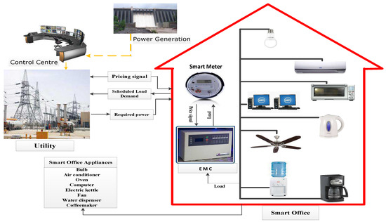
Figure 1.
The proposed system model architecture.
The scheduled vector of office energy consumption (OEC) for a single appliance is:
Total energy consumption is calculated as:
Table 1 gives the specifications of different appliances in an office.

Table 1.
Specifications of office automatically operating appliances (AOAs).
4.2. Problem Formulation
In the proposed work, we formulate our problems of: (a) end-user high comfort level, (b) consumers’ electricity bill minimization and (c) minimization of PAR by optimization of the energy consumption profiles of office appliances, using the multiple knapsack problem (MKP) scheduling technique. MKP is a capacity (resources) allotment problem. It consists of N number of capacities and Q number of objects [28].
MKP is a combinatorial problem. In MKP, the stuff quantity, having different weights and values, can be kept into a knapsack of a certain capacity, such that the worth of the knapsack should be maximum, as shown in Figure 2.

Figure 2.
The multiple knapsack problem (MKP) formulation.
We consider U number of knapsacks and use MKP as the scheduling mechanism to map our problem as follows:
- Power capacities of consumers in every time interval are mapped as U number of knapsacks;
- Appliances in an office are mapped as “Q” number of objects;
- The weight of every object in MKP is mapped as appliances’ consumed energy in every time interval. This is assumed to be time invariant;
- In MKP, the worth of each object in a particular time interval is mapped as the cost of appliances’ consumed energy in that interval of time [29].
If is the maximum energy capacity in every time slot, then the end-user electricity cost along with PAR can be minimized, keeping aggregated energy consumption of the cumulative office appliances within the maximum threshold limit of .
Mathematically, this constraint can be shown as follows:
Here, is the cumulative energy demand of the end-user and is the maximum energy capacity in a particular interval of time available from the utility grid. MKP scheduling tells us to keep the total energy demand of the end-user less than or equal to this maximum energy capacity threshold.
4.3. The Electricity Cost
In order to calculate total energy cost, we use the following equation:
C is the total cost in 60 time slots; is the energy cost per hour; is the connected appliances’ power rating.
4.4. The Power Consumption
The power consumption of each appliance is calculated by the following equation:
is the power rating, and X is the ON/OFF status of an appliance.
4.5. PAR
For RAR, the following equation is used.
4.6. Waiting Time
This is that time interval when a consumer wants to switch-ON an appliance. However, due to the scheduling of appliances, the consumer has to wait for a certain amount of time. Figure 3 shows that is the appliance starting time, but actually, the appliance will start its operation at . mathematically, the waiting time is given as:
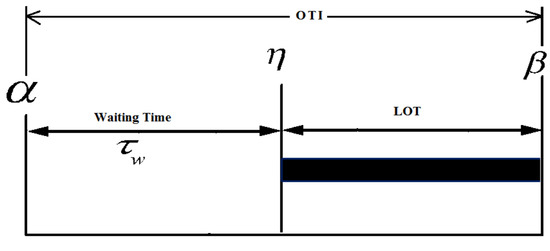
Figure 3.
Appliances starting time, operation ending time and waiting time.
The normalized waiting time is given by:
where is the last starting time of an appliance, so that it will complete its operation.
4.7. Objective Function
Our objective function can mathematically be expressed as follows:
where is the energy cost in every interval of time. The aim of our objective function is to minimize electricity cost, while keeping a higher consumer comfort level by the reduction of waiting time. and are weighting factors of the two portions of our objective function. Their values can be either “0” or “1”, so that ( + ) = 1 [9]. This reveals that either or could be zero or one. This means that, if a consumer does not want to schedule his/her appliances, then these weighting factors will be = 1 and = 0 in the objective function.
5. Scheduling Algorithms
To solve the appliances optimal scheduling problem, in order to achieve the lowest energy cost, lower PAR and less user discomfort, different scheduling algorithms have been proposed in the literature. In this paper, we have proposed GOA and BFA. A brief description of both of these algorithms is given below.
5.1. Grasshopper Optimization Algorithm
A grasshopper is a kind of destructive insect, which is known as a pest because it damages crops. There are eleven thousand species of grasshopper [30]. It is generally considered as a flying animal. As a grasshopper reaches its adult stage, it passes through the stages of eggs, nymph and adult, as shown in the Figure 4.
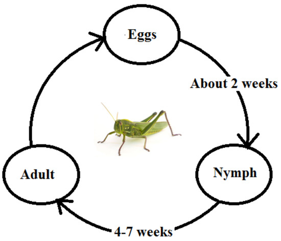
Figure 4.
The lifecycle of a grasshopper.
Usually, grasshoppers can be seen in the form of a swarm in nature. They attack agricultural lands and become a nightmare for formers. The swarming behaviour is found in both adult and nymph grasshoppers [31,32]. Generally, a locust swarm contains five billion of grasshoppers and spread over an area of 60 square miles. Nature-inspired algorithms have a unique search mechanism for food. This consists of two techniques: exploration and exploitation.
(a) Exploration: The process in which the algorithm finds a new solution from the current solutions in the search space.
(b) Exploitation: The process in which algorithm searches the surrounding search space.
The mathematical model of GOA, which carries the swarming behaviour of a grasshopper, is given as in [33].
In the above equation, shows the position of a grasshopper, gives the social collaboration, gives the gravitational force over a grasshopper and is the air-advection. To produce randomness in the above equation, it becomes:
where and are random numbers between zero and one. is modelled as:
where N is the number of search agents, s defines the social interaction between two grasshoppers i and j, is the respective distance between and grasshoppers and is given by:
and:
is the unit vector from the grasshopper to the grasshopper. Mathematically, the social force is given as follows:
where F is the attractive force, d shows the distance and l is the measure of attraction.
The V component in Equation (1) is given as:
where v is the gravitational force, and the negative sign shows its direction towards the centre of the Earth, while is the unit vector in the direction of the Earth.
Now, the A component in Equation (1) is given as:
where v is the constant drift when there is a wind and shows the wind directional unit vector. By putting the values of S, G and A in Equation (1), we get:
We utilize the above equation for the swarm in free space and use it in simulation to describe the interaction between the grasshoppers in a swarm. The steps involved in the GOA algorithm are given in Algorithm 1 and are depicted in Figure 5.
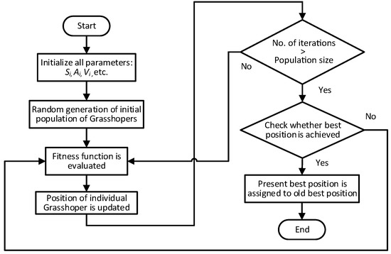
Figure 5.
Flowchart of grasshopper optimization algorithm (GOA).
| Algorithm 1: GOA algorithm. |
 |
5.2. Bacterial Foraging Algorithm
BFA was proposed by Kevin Passino in 2002 [34]. In this algorithm, the group foraging strategy of a swarm of Escherichia coli (E. coli) bacteria is the key point. Bacteria forage for food and nutrients, to maximize their energy per unit time. By sending a signal, bacteria also communicate with each other. Because of predators, the prey may be mobile. Therefore, it is chased by the bacterium in an optimal way. When a bacterium maximizes its energy by getting sufficient food, then it does other activities like sheltering, mating, fighting, etc.
The following steps are needed in order to explain BFA.
- (a)
- Chemotaxis
- (b)
- Swarming
- (c)
- Reproduction
- (d)
- Elimination
5.2.1. Chemotaxis
In the chemotaxis step, the E. coli move from one place to another through flagella. According to the biological point of view, its motion is observed in two different ways: it may either swim or tumble.
To consider the chemotaxis movement of bacteria, we have the following equation:
In the above equation, shows the position of the bacterium at the chemotactic, the reproductive and the elimination-dispersal step. represents the size of the step taken by the bacterium in a random direction when it tumbles. shows the vector in random direction [−1, 1].
5.2.2. Swarming
The E. coli bacterium is blessed with swarming behaviour. In this step, bacteria cells form a ring-shaped structure and move in search of nutrients. A high level of succinate usage stimulates the cells, due to which attractant-aspartate is released by the cells, which helps them to bind in groups.
5.2.3. Reproduction
When a bacterium is in a feasible and nutritious environment, it reproduces, splits into two bacteria and keeps the number of cells in a swarm fixed.
5.2.4. Elimination and Dispersal
The scarcity of nutrients kills the bacterium or disperses them into another environment. They are also killed due to high temperature. If there is a poor condition in the environment, the bacteria may place themselves near a good food source, hence assisting chemotaxis.
To calculate the fitness of each bacterium, the following equation can be used:
In the above equation, shows the fitness of the bacterium and is the position of the bacterium.
In order to achieve the time-varying objective, we must put the objective function into the actual objective function . The steps involved in the BFA algorithm are given in Algorithm 2 and are depicted in Figure 6.
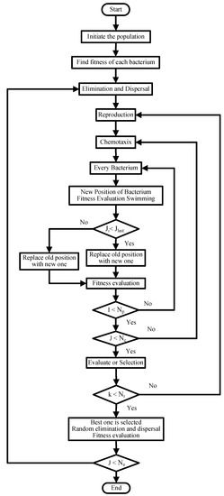
Figure 6.
Flowchart of bacterial foraging algorithm (BFA).
| Algorithm 2: Bacterial foraging algorithm. |
 |
6. Simulation Results
A substantial simulation was performed to show the performance of different algorithms in terms of minimization of electricity cost by shifting appliances from on-peak hours to off-peak hours, minimization of PAR and minimization of end-user discomfort due to waiting time. In this paper, eight appliances were selected, as shown in the Table 1. For comparison purpose, firefly algorithm (FA), cuckoo search algorithm (CSA) and ant colony optimization algorthm (ACO) are considered in the same scenario for thirty-days load scheduling. Figure 7 gives the day-ahead pricing (DAP) signal, taken from the daily report of the New York Independent System Operator (NYISO) [35]. The total time of 24 h was divided into 24 time slots. For an office, usually 8–12 h was used, so time was taken from 8:00–20:00. Figure 8 shows the daily unscheduled load and scheduled load with the GOA and BFA algorithms. The figure shows that GOA outperformed by eliminating the peak in the unscheduled load. Figure 9 shows the hourly unscheduled (Un-sch) and scheduled load with GOA and BFA cost. It is clear that the hourly cost is averaged compared to the unscheduled cost, especially the high cost in the on-peak hours due to shifting of the load from on-peak hours to off-peak hours. Figure 10 shows that the office monthly load was equal for all algorithms, as each algorithm had to reschedule the appliances only. Figure 11 depicts the total monthly cost in dollars. In the unscheduled case, we had a maximum cost of 267.45 $; when scheduled by GOA, it became 174.67 $ (34.69% reduction); and in the case of BFA, it became 161.23 $ (37.47% reduction). The comparison of these proposed algorithms with state-of-the-art algorithms for the same scenario is depicted in Table 2. Figure 12 depicts the daily PAR. It is clear from the figure that our proposed schemes minimized the PAR. Before scheduling, the PAR value was 7.81, and after scheduling with GOA and BFA, the PAR values became 3.42 (56.20% reduction) and 6.18 (20.87% reduction), respectively. Figure 13 depicts the average waiting time. The waiting time in the case of GOA was 1.28 h, and BFA was 1.32 h. This shows that the waiting time of BFA was greater than GOA because it had reduced the total cost more than that reduced by BFA. Table 2 shows that, there is always a trade-off between energy cost and waiting time.
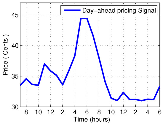
Figure 7.
Day-ahead pricing signal [35].
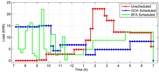
Figure 8.
Hourly load for unscheduled load and scheduled load with the GOA and BFA algorithms.
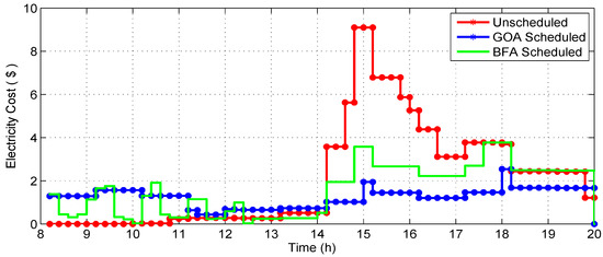
Figure 9.
Hourly cost for unscheduled load and scheduled load with the GOA and BFA algorithms.
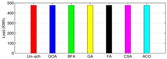
Figure 10.
Total monthly load.
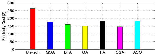
Figure 11.
Total cost.
Table 2.
Comparison of the unscheduled load and scheduled load with the GOA, BFA, GA, FA, CSA and ACO algorithms.
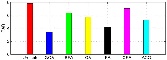
Figure 12.
The peak-to-average power ratio (PAR).
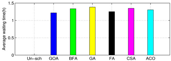
Figure 13.
Average waiting time.
Table 2 compares the performance of the proposed algorithms with unscheduled load and state-of-the-art algorithms like firefly algorithm (FA), cuckoo search algorithm (CSA) and ant colony optimization (ACO) with respect to three parameters; energy cost, waiting time and PAR.
Table 3 shows the run-time of the proposed algorithms using an Intel (R) Core (TM) i5 processor, with 4.00 GB of installed memory (RAM) and the 32-bit Windows 7 Operating system.
Table 3.
Run-time of the proposed algorithms for 30 days of load scheduling.
7. Conclusions
In this paper, we have proposed a novel technique of appliances’ scheduling in an office. We used two nature-inspired optimization algorithms, GOA and BFA, to achieve our objective functions of end-user electricity bill minimization along with a reduction of PAR and user discomfort due to appliance scheduling. We considered only eight appliances to check our proposed algorithms’ performance. We compared our results with a few state-of-the-art nature-inspired algorithms in the literature like GA, FA, CSA and ACO for the three mentioned fitness functions, i.e., minimization of the electricity bill, PAR and waiting time. Indeed, numerous countries in the world can fulfil electricity demand. However, keeping in view the minimization of the electricity bill, the reliability of the existing system and improvements towards smart grids to facilitate the customers, with increased dependency on electricity with automation, energy optimization is a big issue throughout the world. Furthermore, with increased electricity generation, carbon emission increases due to the use of different types of fuels, which pollute this biosphere day by day. Therefore, the advantage of these algorithms for energy optimization is not only to save money, but to reduce pollution, as well. The simulation results show that our proposed energy optimization schemes performed well in the case of minimization of PAR and cost. However, when energy cost is minimized, user waiting time will increase as a penalty. In the future, multi-objective algorithms will be designed to minimize the energy cost and PAR while keeping in view the high comfort level of consumers. Furthermore, the proposed algorithms will be applied to residential, commercial and industrial areas for the greater benefit of both the utility and consumers. For this purpose, more nature-inspired algorithms will be used and analyzed.
Author Contributions
I.U. proposed the idea and did the writing, review and editing; Z.K. did the formal analysis and comparisons; M.N.K. proposed the topology and system design; S.H. provided technical supervision, insights and additional ideas on the presentation. All authors equally contributed, revised and approved the manuscript.
Funding
This research received no external funding.
Conflicts of Interest
The authors declare no conflict of interest.
Abbreviations
The following abbreviations are used in this manuscript:
| OEC | Office energy consumption |
| LOT | Length of operational time |
| OTI | Operational time interval |
| AOAs | Automatically operating appliances |
| PAR | Peak-to-average power ratio |
| Un-sch | Un-scheduled load |
| FA | Firefly algorithm |
| CSA | Cuckoo search algorithm |
| ACO | Ant colony optimization |
| s | Each time slot |
| C | The total electricity cost in sixty time slots |
| Power rating of connected appliances | |
| Power consumption of each appliance | |
| Waiting time for an appliance | |
| S | Set of 60 time slots |
| Energy cost per hour | |
| X | ON-OFF states of an appliance |
| Starting time of an appliance | |
| Operational starting time of an appliance | |
| Ending time of an appliance |
References
- Hashmi, M.; Hnninen, S.; Mki, K. Survey of smart grid concepts, architectures, and technological demonstrations world-wide. In Proceedings of the IEEE PES Conference on Innovative Smart Grid Technologies (ISGT Latin America), Medellin, Colombia, 19–21 October 2011; pp. 1–7. [Google Scholar]
- Rahimi, F.; Ipakchi, A. Demand response as a market resource under the smart grid paradigm. IEEE Trans. Smart Grid 2010, 1, 82–88. [Google Scholar] [CrossRef]
- Ahmed, A.; Manzoor, A.; Khan, A.; Zeb, A.; Ahmad, H. Performance Measurement of Energy Management Controller Using Heuristic Techniques. In Proceedings of the Conference on Complex, Intelligent, and Software Intensive Systems, Turin, Italy, 10–13 July 2017; pp. 181–188. [Google Scholar]
- Ozturk, Y.; Senthilkumar, D.; Kumar, S.; Lee, G. An intelligent home energy management system to improve demand response. IEEE Trans. Smart Grid 2013, 4, 694–701. [Google Scholar] [CrossRef]
- Mavrotas, G.; Karmellos, M. Multi-objective optimization and comparison framework for the design of Distributed Energy Systems. Energy Convers. Manag. 2019, 180, 473–495. [Google Scholar]
- Sousa, T.; Morais, H.; Vale, Z.; Faria, P.; Soares, J. Intelligent energy resource management considering vehicle-to-grid: A simulated annealing approach. IEEE Trans. Smart Grid 2012, 3, 535–542. [Google Scholar] [CrossRef]
- Soares, J.; Sousa, T.; Morais, H.; Vale, Z.; Faria, P. An optimal scheduling problem in distribution networks considering V2G. In Proceedings of the IEEE Symposium on Computational Intelligence Applications in Smart Grid (CIASG), Paris, France, 11–15 April 2011; pp. 1–8. [Google Scholar]
- Tsui, K.M.; Chan, S.C. Demand response optimization for smart home scheduling under real-time pricing. IEEE Trans. Smart Grid 2012, 3, 1812–1821. [Google Scholar] [CrossRef]
- Zhao, Z.; Lee, W.C.; Shin, Y.; Song, K.B. An optimal power scheduling method for demand response in home energy management system. IEEE Trans. Smart Grid 2013, 4, 1391–1400. [Google Scholar] [CrossRef]
- Arabali, A.; Ghofrani, M.; Etezadi-Amoli, M.; Fadali, M.S.; Baghzouz, Y. Genetic-algorithm-based optimization approach for energy management. IEEE Trans. Power Deliv. 2013, 28, 162–170. [Google Scholar] [CrossRef]
- Tang, L.; Zhao, Y.; Liu, J. An improved differential evolution algorithm for practical dynamic scheduling in steelmaking-continuous casting production. IEEE Trans. Evol. Comput. 2014, 18, 209–225. [Google Scholar] [CrossRef]
- Liu, B.; Kang, J.; Jiang, N.; Jing, Y. Cost control of the transmission congestion management in electricity systems based on ant colony algorithm. Energy Power Eng. 2011, 3, 17. [Google Scholar] [CrossRef]
- Khalid, A.; Javaid, N.; Mateen, A.; Khalid, B.; Khan, Z.A.; Qasim, U. Demand Side Management using Hybrid Bacterial Foraging and Genetic Algorithm Optimization Techniques. In Proceedings of the 10th International Conference on Complex, Intelligent, and Software Intensive Systems (CISIS), Fukuoka, Japan, 6–8 July 2016; pp. 494–502. [Google Scholar]
- Wang, K.; Li, H.; Maharjan, S.; Zhang, Y.; Guo, S. Green Energy Scheduling for Demand Side Management in the Smart Grid. IEEE Trans. Green Commun. Netw. 2018, 2, 596–611. [Google Scholar] [CrossRef]
- Ullah, I.; Hussain, S. Time-Constrained Nature-Inspired Optimization Algorithms for an Efficient Energy Management System in Smart Homes and Buildings. Appl. Sci. 2019, 9, 792. [Google Scholar] [CrossRef]
- Aslam, S.; Bukhsh, R.; Khalid, A.; Javaid, N.; Ullah, I.; Fatima, I. An Efficient Home Energy Management Scheme Using Cuckoo Search. In Proceedings of the International Conference on P2P, Parallel, Grid, Cloud and Internet Computing, Taichung, Taiwan, 27–29 October 2018; pp. 167–178. [Google Scholar]
- Yang, X.-S.; Suash, D. Cuckoo search via Lévy flights. In Proceedings of the 2009 World Congress on Nature & Biologically Inspired Computing (NaBIC), Coimbatore, India, 9–11 December 2009; pp. 210–214. [Google Scholar]
- Manzoor, A.; Javaid, N.; Ullah, I.; Abdul, W.; Almogren, A.; Alamri, A. An Intelligent Hybrid Heuristic Scheme for Smart Metering based Demand Side Management in Smart Homes. Energies 2017, 10, 1258. [Google Scholar] [CrossRef]
- Gao, R.; Wu, J.; Hu, W.; Zhang, Y. An improved ABC algorithm for energy management of microgrid. Int. J. Comput. Commun. Control 2018, 13, 477–491. [Google Scholar] [CrossRef]
- Shirazi, E.; Jadid, S. Optimal residential appliance scheduling under dynamic pricing scheme via HEMDAS. Energy Build. 2015, 93, 40–49. [Google Scholar] [CrossRef]
- Adika, C.O.; Wang, L. Smart charging and appliance scheduling approaches to DSM. Int. J. Electr. Power Energy Syst. 2014, 57, 232–240. [Google Scholar] [CrossRef]
- Huang, Y.; Wang, L.; Guo, W.; Kang, Q.; Wu, Q. Chance Constrained Optimization in a Home Energy Management System. IEEE Trans. Smart Grid 2018, 9, 252–260. [Google Scholar] [CrossRef]
- Javaid, N.; Hussain, S.M.; Ullah, I.; Noor, M.A.; Abdul, W. Demand Side Management in Nearly Zero Energy Buildings Using Heuristic Optimizations. Energies 2017, 10, 1131. [Google Scholar] [CrossRef]
- Ma, K.; Hu, S.; Yang, J.; Xu, X.; Guan, X. Appliances scheduling via cooperative multi-swarm PSO under day-ahead prices and photovoltaic generation. Appl. Soft Comput. 2018, 62, 504–513. [Google Scholar] [CrossRef]
- Asgher, U.; Rasheed, B.; Saad, A.; Rahman, A.; Alamri, A. Smart Energy Optimization Using Heuristic Algorithm in Smart Grid with Integration of Solar Energy Sources. Energies 2018, 11, 3494. [Google Scholar] [CrossRef]
- Bharathi, C.; Rekha, D.; Vijayakumar, V. Genetic Algorithm Based Demand Side Management for Smart Grid. Wirel. Pers. Commun. 2017, 93, 481–502. [Google Scholar] [CrossRef]
- Shi, K.; Li, D.; Gong, T.; Dong, M.; Gong, F.; Sun, Y. Smart Community Energy Cost Optimization Taking User Comfort Level and Renewable Energy Consumption Rate into Consideration. Processes 2019, 7, 63. [Google Scholar] [CrossRef]
- Liu, Y.; Yuen, C.; Huang, S. Peak-to-Average Ratio Constrained Demand-Side Management with Consumer’s Preference in Residential Smart Grid. IEEE J. Sel. Top. Signal Process. 2014, 8, 1084–1097. [Google Scholar] [CrossRef]
- Yang, X.S. Firefly algorithms for multimodal optimization, in Stochastic Algorithms: Foundations and Applications. Lect. Notes Comput. Sci. 2009, 5792, 169–178. [Google Scholar]
- Saremi, S.; Mirjalili, S.; Lewis, A. Grasshopper optimization algorithm: Theory and application. Adv. Eng. Softw. 2017, 105, 30–47. [Google Scholar] [CrossRef]
- Simpson, S.J.; McCaffery, A.; HAeGELE, B.F. A behavioural analysis of phase change in the desert locust. Biol. Rev. 1999, 74, 461–480. [Google Scholar] [CrossRef]
- Rogers, S.M.; Matheson, T.; Despland, E.; Dodgson, T.; Burrows, M.; Simpson, S.J. Mechanistically-induced behavioural gregarization in the desert locust Schistocerca gregaria. J. Exp. Biol. 2003, 206, 3991–4002. [Google Scholar] [CrossRef] [PubMed]
- Topaz, C.M.; Bernoff, A.J.; Logan, S.; Toolson, W. A model for rolling swarms of locusts. Eur. Phys. J. Spec. Top. 2008, 157, 93–109. [Google Scholar] [CrossRef]
- Passino, K.M. Biomimicry of bacterial foraging for distributed optimization and control. IEEE Control Syst. 2002, 22, 52–67. [Google Scholar]
- Day-Ahead Pricing (DAP). NYISO (New York Independent System Operator). Available online: http://www.energyonline.com/Data/GenericData.aspx?DataId=11&NYISO-Day-Ahead-Energy-Price (accessed on 25 January 2019).
© 2019 by the authors. Licensee MDPI, Basel, Switzerland. This article is an open access article distributed under the terms and conditions of the Creative Commons Attribution (CC BY) license (http://creativecommons.org/licenses/by/4.0/).