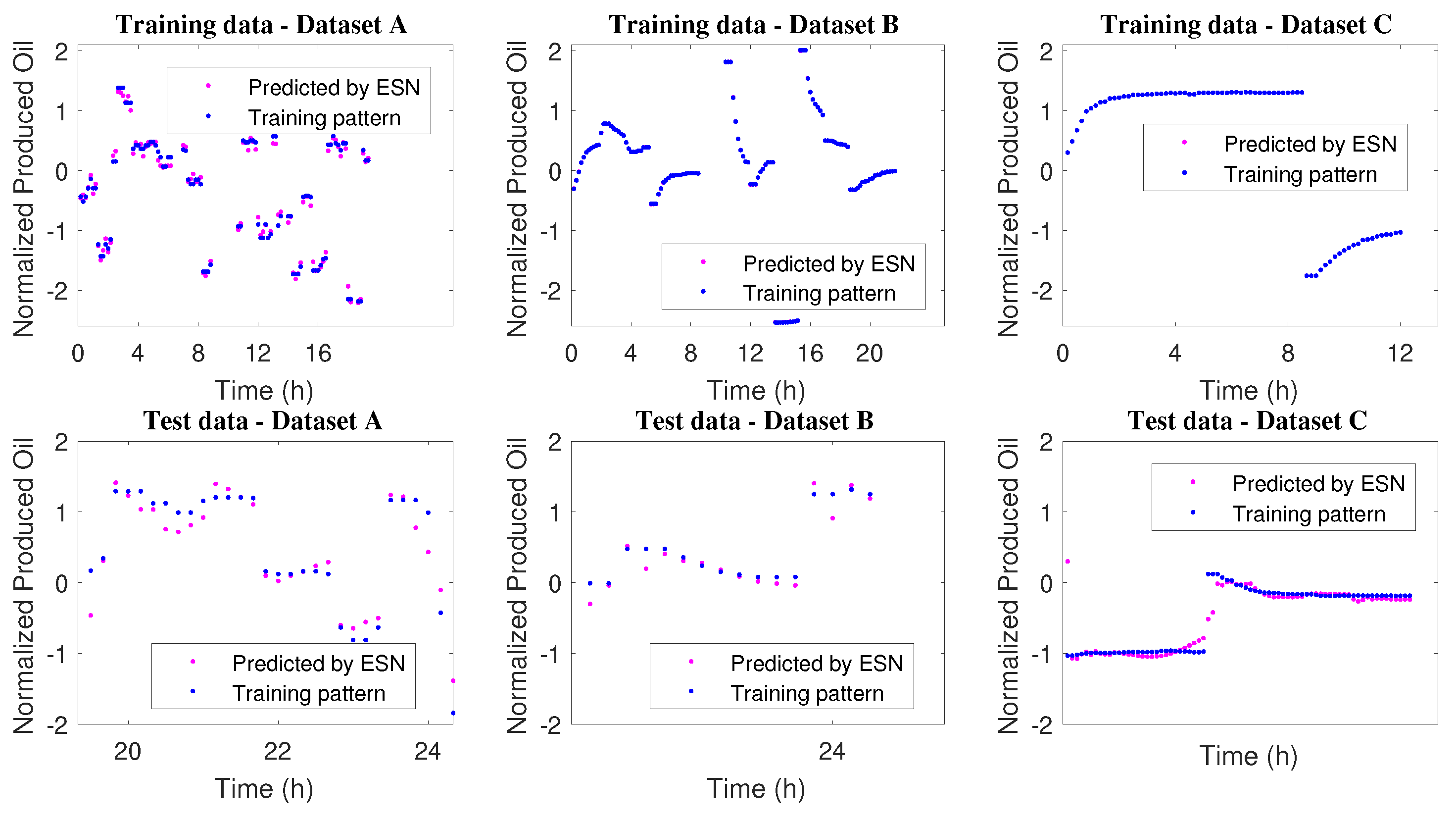
Abstract
The present work investigated the use of an echo state network for a gas lift oil well. The main contribution is the evaluation of the network performance under conditions normally faced in a real production system: noisy measurements, unmeasurable disturbances, sluggish behavior and model mismatch. The main pursued objective was to verify if this tool is suitable to compose a predictive control scheme for the analyzed operation. A simpler model was used to train the neural network and a more accurate process model was used to generate time series for validation. The system performance was investigated with distinct sample sizes for training, test and validation procedures and prediction horizons. The performance of the designed ESN was characterized in terms of slugging, setpoint changes and unmeasurable disturbances. It was observed that the size and the dynamic content of the training set tightly affected the network performance. However, for data sets with reasonable information contents, the obtained ESN performance could be regarded as very good, even when longer prediction horizons were proposed.
1. Introduction
Control structures allow connections between different equipment and processes and the implementation of reference values, reducing the variability and minimizing the effect of disturbances throughout the process. When satisfactorily designed, they ensure the efficient and safe operation. Classical Proportional Integral Derivative (PID) controllers are the ones used most often in the industry, representing at least 95% of the regulatory control loops in operation [1]. These controllers exhibit many advantages, like robustness and simple design. Furthermore, PID controllers require few tuning parameters (three when all modes are available: proportional, integral and derivative), with well-known effects on the control system, which allows the operator to have complete knowledge of the system responses for simple applications (Single-Input Single-Output (SISO) , linear processes). However, the technological advances have made industrial plants more complex and integrated, with high dimensions and strong non-linearities, requiring a more holistic treatment of the process. In these more complicated scenarios, conventional descentralized control strategies, such as PIDs, may fail, mainly because coupling among the possibly many process variables is not taken into account. Additionally, improvements of transmission, storage and information processing capacities of process computers led to the significant increase of the interest in advanced control strategies [1,2,3,4].
Model predictive control (MPC) is the most popular approach for advanced control. It encompasses a wide range of algorithms that, by using a process model and optimization tools, determine the control actions, for each sampling instant, considering the current states of the plant and open-loop time horizon predictions. These tools constitute standard and well-established techniques that make possible to deal with input and output constraints, interactions among process variables and, when based on a nonlinear model (as is the case in the Nonlinear Model Predicitve Control or NMPC), strong nonlinearities. The main differences between algorithms regard the type of employed model, representation of disturbances and operational constraints, and the objective function used to perform the optimization step [5].
The design of model-based methods starts with the system identification/modeling approach and then with the development of the control rule that is founded on the premise that the model truly represents the plant behavior [1]. First principles model building involves simplification, abstraction, calculation, programming, simulation, and interpretation steps. This kind of model is very difficult to obtain, and it is usually impossible to describe every phenomenon involved on the process. Most MPC industrial packages contain a set of models that predict latent variables (from available measurements) and future plant behavior. However, the reliability of the controller depends on the ability of the plant model to capture the process behavior. This could be a problem because, after some operating time, plant conditions deviate from the design conditions and some unmodeled dynamics and, consequently, modeling errors may show up. For this reason, periodic evaluations (and updates) are necessary to ensure the predictive power of these models. This step is generally performed offline and requires an expert operator to ensure the reliability of the MPC, being this the greatest difficulty faced by users [1,6].
The re-identification step, performed by a non-expert operator, during maintenance of the MPC, can lead to poor models [6]. As a consequence, the performance of model-based tools can be less robust and safe. The plant-model mismatch also affects the stability and convergence of the controller. Even when the set of models is considered to be sufficiently accurate, the results of stability, convergence and robustness still may present problems whenever the assumptions made about the system deviate from practical reality [1,6]. So, even when there is the possibility of obtaining a model, important issues remain open regarding: how long the model can be regarded as adequate for representation of the process behavior and how stability of the resulting controller can be ensured.
These difficulties and questionings related to identification of models used in predictive control approaches stimulated the search for alternative strategies. In addition, with the increasing connectivity and availability of cheaper sensors, the amount of daily generated measured variables has changed from hundreds to thousands of variables. This new scenario can be observed in all sectors and gave birth to a new paradigm: the Big Data Era [7,8,9].
Big Data can be defined by much more than massive amount of data; it can be related to the famous Vs: Volume, Variety, Velocity, Veracity and Value. However the real concept and understanding of this trend is much broader. It is related to today’s technological advancements and all its consequences, including device miniaturization, large storage and processing capacity, cost reduction of technological supplies (CPUs and memories), process automation and virtualization. In this new era, the widespread use of equipment for production, storage, processing, connectivity, among other tasks, is observed. Hence, Big Data goes beyond generating a large mass of data, storing it and processing it in servers and clusters; it represents a cultural and social paradigm shift, and also a phase of the contemporary industrial revolution, the so called Industry 4.0 [9,10].
The currently easy internet access and the growth of the so-called Cloud Computing and Internet of Things (IoT) reinforce some of the Big Data issues. Sensors spread all over the world generate and transmit in real time, which can be stored and processed in the cloud. This large volume and variety of data has boosted research in data science, focusing on data-based techniques and analytics. From the industrial process point of view, the set of off-line data carries important information about the system and can provide the knowledge required to build models used to represent the controlled system; design the controller and, by means of data processing and mining techniques, improve the control performance. Besides, models can also be used for prediction and evaluation of the future behavior of the system. The set of on-line data reflects, in real time, disturbances and changes in the process, allowing the controller to notice process alterations in time for action and correction. In conclusion, the available data and the techniques available for data handling can be used to increase our knowledge about the systems [7,9].
The knowledge driven modeling approach uses the prior knowledge of the process to provide refined analyses and decisions. In contrast, data-driven approaches are quicker and do not require extensive modeling efforts [11]. These methodologies became new trends on Process Control at the end of the 1990s, being the theme of study in several research groups [3]. So, new paradigms that can be used to extract the process dynamic behavior from historical databases and allow on line modifications on the plant model have gained prominence [1,7]. However, they can lead to super-parameterized modeling and should be used with great caution, as this large volume of data can lead to overfitting. Thus, there is strong interest in developing robust and integrated methods, based on combined data-driven and model-driven approaches for control, optimization, planning and management of industrial systems [3,12,13].
Artificial neural networks are one of the most used data-driven approaches. Their processing structures are inspired by the fault tolerant parallel processing capability of the biological nervous system. They exhibit exceptional features, such as adaptability and input-output mapping capabilities, and can be easily assembled through integration among simple processing units (neurons). By nature, they are multivariable, dealing with complex, high-dimensional problems with multiple inputs and outputs. Due to these attractive characteristics, these structures have been widely applied in chemical processes over the years [14,15].
The main contribution of the present manuscript is the investigation and use, as a predictive model, of a special type of neural network which explores the temporal nature of data, the echo state network or esn [16], in the presence of plant-model mismatch. With that purpose, the robustness of the developed esn model is evaluated under different scenarios that simulate changes in the plant. The chosen plant for the evaluation of the proposed tool is the gas lift oil well process, which configures an important control problem due to the inherent system characteristics, including static gain signal inversion, nonminimum phase behavior, slow transient response and possible open loop instabilities. As will be fully shown ahead, data of gas lift oil well plant operation was generated by simulation using different first principles models. Then esn models were developed and tested based on these data, allowing the study of the generalization ability of the esn model for operation under different conditions. The use of simulation of rigorous models allows the elaboration of an efficient methodology for generating data for training esn for such processes, as different situations are focused (for instance, the definition of the level of excitation of the input variables). The final target is that this methodology may be further applied to real processes in the oil industry.
The paper is organized as follows: in Section 2 we present some important considerations about Neural Networks, highlighting the Echo State Network; in Section 3 we describe the mathematical models used to represent the gas-lift well considered in the present work; in Section 4 we design the esn model and use it to perform some open-loop simulations; in Section 5 we present the results concerning the possible implementation of the proposed model in a real production environment. The conclusions of the present work are summarized in Section 6.
2. Echo State Network
The forecasting of future events constitutes a relevant task on the fields of process modeling and control. In the particular field of chemical processes, due to intrinsic difficulties related to phenomenological modeling, many situations require the prediction of the future plant behavior based on current and past available information. Prediction algorithms need to extract the correlation dynamics from related events to anticipate the next (or a horizon of) results. In this context, machine learning algorithms are iterative and “learn” by recognizing patterns from observed data. When exposed to a new set of data, many machine learning procedures can adapt automatically. For this reason, the range of possible applications for chemical processes is extensive. As a consequence, it is not surprising to observe that these procedures have been widely used for process modeling, fault identification, variable estimation, among many other possible applications. Among the many existing algorithms, we can highlight artificial neural networks (ANN), support vector machine-based methods (SVM), partial least squares regression (PLS) methods and fuzzy logic algorithms, which have been extensively used in recent years [14,17,18,19,20,21].
ANNs are techniques inspired in biological neural networks and their ability to learn from the environment and to make that knowledge available for use. They constitute parallel distributed paradigms, consisting of many simple processing units, the artificial neurons, interconnected and organized in layers. The input signals from the external environment (or from previous neurons) are multiplied by their respective synaptic weights, simulating the synapses that occur in the biological systems. After multiplication by weights, the weighted information is added to a bias parameter, and the result is modified by an activation function, which generates the output signal of the artificial neuron, as shown in Equations (1) and (2), for a network with one non-linear hidden layer and a linear output layer. Then, the signal is transmitted to the external environment or, in the case of multiple hidden layers, to the neurons in the next layer. The bias has the effect of increasing or decreasing the network input of the activation function, depending on whether it is positive or negative, respectively [15].
The subscript i represents the hidden neuron while j represents the output neuron; represents the weghting matrix, so that is the i-th line of the weight matrix between the inputs and hidden layers and is the j-th line of the weight matrix between the hidden and output layers; b, the bias; , the internal states vector; the external inputs vector and f is a non-linear function applied for each element of the hidden layer. A neural network works with multiple neurons organized in sequenced layers. The data is fed into the input layer and the network response to its effect is observed at the output layer. Information can be propagated in a network in two ways: from incoming neurons, through hidden neurons, to outgoing neurons; or from the exit of a neuron from the next layer to a neuron in the precedent layer, or even to the neuron itself [15,17,18].
A network is classified as feedforward when it does not work with any information loop. It is then a static network, so that from a set of inputs, it can only predict a set of outputs, without carrying any memory about the process dynamics. A network is classified as feedback when it presents loops (recurrence) of information. The feedback architecture enables memorizing temporally information. These feedback networks, also called Recurrent Neural Networks (RNN), are better suited to deal with time series due to their memory ability, hence they are expected to play an important role in the Big Data Era, typically characterized by the availability of large volume and variety of process data. Beyond their dynamic memory ability, the RNN architecture enables another important feature: a high capacity of adaptation [22,23]. Equations (3) and (4) show the update step for a simple recurrent network.
The data are fed into the input layer and are propagated to the output layer; however, they can also flow among previous layers. The subscript k is related to the instant of time when the data is informed to the network.
The most popular way to train a neural network is the backpropagation method; however, loops and discontinuity at some points of the space (bifurcations points) of the ANN can hinder the proper training and make it non-converging, computationally expensive and lead to poor local minima [18,23,24].
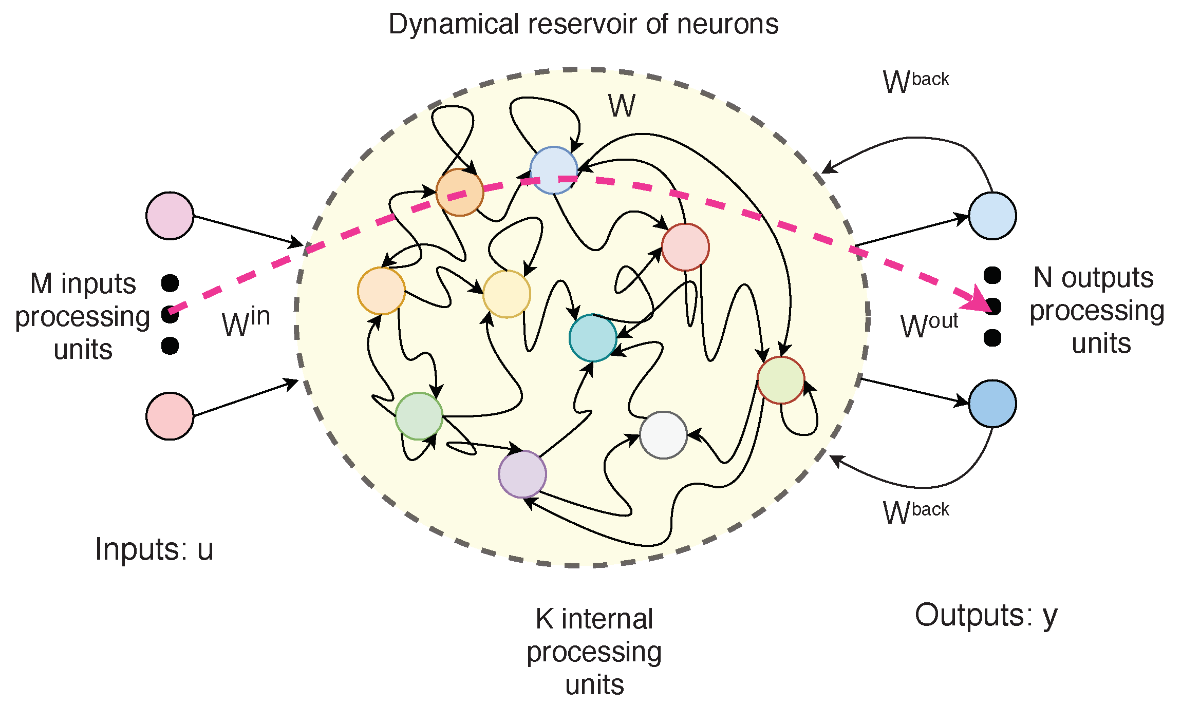
Echo State Networks (ESN) are special types of RNN developed by Jaeger [16]. They are composed of an input layer, a reservoir of recurrently organized neurons and an output layer. Figure 1 shows a simplified representation of the ESN structure.
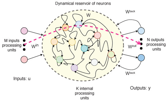
Figure 1.
A simplified representation of the ESN structure.
The reservoir, which is composed by many sparsely connected neurons, provides the network with a temporal memory, processing the information in a dynamic context. However, the training is performed only with the weights of the reservoir output neurons, which avoids the problems of convergence and computational cost of other ANN training procedures. Only the weights of the reservoir outputs are accounted and adjusted to the patterns and a simple linear regression can be used with that purpose. The low computational cost and the capacity to deal with large data volumes make them suitable for Big Data contexts. On the other hand, distinct global parameters influence the generation of the reservoir, so that the success of applications requires some user experience [23,25]. The typical updating equations governing the reservoir is given by Equation (5) and the output is computed with Equation (6).
where represents the n-dimensional reservoir activation state vector, is the vector of external inputs and is the output vector. is the internal state activation function vector, commonly the hyperbolic tangent function. is the leak rate and is correlated to the network memory ability. is the post-processing activation function vector, commonly considered as the identity function. is the input connection (weight) matrix, represents the reservoir recurrence and are the weights for readout output layer. Besides , the ESN design requires the tuning of other parameters, frequently called “metaparameters”, because they do not really represent weights and connections, but confer the characteristics of the reservoir and need to be carefully determined. The metaparameters are: reservoir size and sparsity, spectral radius, nonzero elements distribution, input matrix scaling and shift.
Neural networks are promising tools and interesting alternatives for cases where phenomenological models are not available. However, they exhibit some drawbacks. They require a large volume and variety of data to produce reliable predictions. Besides that, there is no guarantee of good generalization ability and, then, training can lead to poor networks. Even though ESN was proposed by Jager [16] almost 20 years ago, only very few works can be found relating ESN and control systems. Huang et al. [25] proposed and evaluated four control schemes: the first based only on an ESN, the second combining the network with PSO (Particle Swarm Optimization) to improve the control, a third scheme which considers a single-layer neural network (SNN) control and a last one that incorporates the improvements of all previous schemes. They considered experiments and simulated results of a Pneumatic Muscle Actuator to show the effectiveness of the new control approach. The convergence and stability of the proposed procedure were guaranteed with rigorous analyses based on the Lyapunov theory. Huang et al. [4] proposed a combined “Echo State” and “Bayesian Inference for Gaussian Processes” predictive control approach and applied it to a Pneumatic Muscle Actuator. The non-linearity, the presence of hysteresis and the existence of time varying parameters make that case study relevant to the control field. The echo state Gaussian process (ESGP) exhibited a good estimation ability and more accurate action than PIDs and Sliding Mode Control.
Regarding applications in the oil-gas industry, Antonelo et al. [11] designed a soft sensor based on ESN for estimation of downhole pressure based on simulations performed with a first-principle model and real data measurements. Results showed that the network robustly modeled the well behavior for slugging and steady steate flow. Jordanou et al. [26] proposed an adaptive controller to the oil well bottom hole pressure through manipulation of the production choque valve opening. The proposed controller used the ESN to explain the inverse model of the well. Another network was used to compute the control action. Results showed that the Echo State based control provided good performance for setpoint tracking and disturbance rejection. Later Jordanou et al. [27] also proposed a model predictive controller that uses ESN for identification purposes. Their scheme is based on combining the ESN with a Practical Nonlinear Model Predictive Controller (PNMPC) and exhibited good performance for setpoint tracking, while obeying the constraints. However a detailed study about the ESN system identification ability, as well as parameter search and studies evolving filtering and controller tuning, have not been performed so far.
3. Gas Lift Well Models
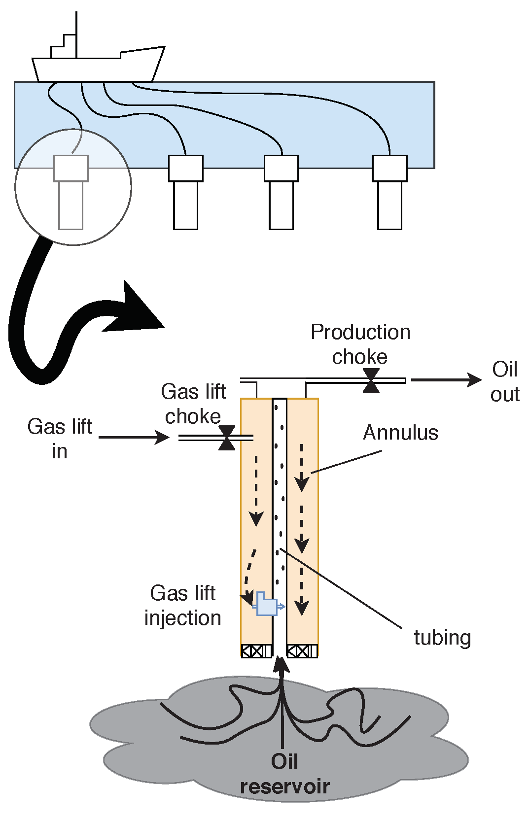
The gas lift injection represents at least 70% of the Brazilian oil production and is also very expressive in respect to the worldwide production [28]. This technique allows the oil and gas extraction in low pressure reservoirs. Gas is injected in the tubing, through the injection valve, and mixes with the fluid. Due to the increase of gas content in the line, the average density of the two-phase fluid mixture is reduced. As a consequence, the hydrostatic pressure gradient also decreases, faciliting the fluid elevation and increasing the well production. Even if the well is dead, the gas lift technology can be applied to recover production [29,30,31]. The injection can be continuous or intermittent, and in this work we consider the continuous gas-lift. Figure 2 shows a simplified representation of the system.

Figure 2.
A simplified representation of the gas-lift oil well system.
During gas lift production, oil wells can present highly oscillatory behavior. This instability is usually undesirable. The oscillatory behavior is not a problem only for financial reasons (losses), but also because it can lead to chaotic, unstable process behavior, and, in extreme cases, it can lead to intermittent production. In addition, large fluctuations in pressure and production rate may limit the overall production, lead to poor separation of oil and gas phases, and cause flaring and shutdown [29,30,32].
Thus, a control system capable of stabilizing the operation, anticipating and preventing intermittent fluctuations from occurring is necessary. The production control is generally performed through manipulation of the injected gas flow, but this control task is challenging due to gain signal inversion, non-minimal phase behavior, slow transient response and possible open loop instabilities [31,33]. These difficulties stimulate the use of advanced control techniques, especially strategies based on predictive control.
There are a few gas lift well models available in the literature, with different levels of detailing. However, even a rigorous phenomenological model provides a simplified process description, given the complexity of the analyzed system. The phenomenological model proposed by Eikrem et al. [34] is a representation of the casing-heading dynamic instability. Ideal gas behavior is assumed and no pressure drop from friction is considered. Oil and water form one single liquid phase with constant mixture properties. The process is assumed to be isothemal and the oil is considered incompressible. Ribeiro [35] included Darcy-Weisbach’s correlation in the model to describe more precisely the pressure drop in the well.
The model presented by Jahanshahi et al. [32] is also based on the work of Eikrem et al. [34], and considers the effects of pressure loss by friction in the well, but in a different way. Besides, a more rigorous approach was used for calculation of the oil and gas fractions and the density at the top of the tubing.
Both models proposed by Eikrem et al. [30] and Jahanshahi et al. [32] assume ideal behavior of the gas phase in the system. However, this hypothesis is not the most suitable in the harsh subsea environment, where pressures are generally high and temperature low. So, in order to consider a more reliable scenario, Rojas Soares et al. [36] proposed the use of the Peng-Robinson Equation of State (EoS) [37] to describe the gas behavior. Table 1 summarizes the particular characteristics of each model.

Table 1.
Particular characteristics of the models.
4. Methodology
The models presented previously describe different levels of detail of the phenomena involved in the gas-lift operation. In particular, all models were used to simulate the real-time process measurements. The model proposed by Eikrem et al. [34] and modified by Ribeiro [35] was used for training of the echo state network and preliminary evaluation of the tool. The prediction tasks were performed based only on historical data (generated by simulation) of the process and on the available online measurement information. The other model, proposed by Jahanshahi et al. [32] and modified by Rojas Soares et al. [36], was used to evaluate the capacity of the network in cases of plant-model mismatch.
Preliminary tests were performed, considering the model proposed by Eikrem et al. [34] and modified by Ribeiro [35], to highlight important characteristics of the process and define the input and output variables for the network. Then the ESN capacity was evaluated in different operational scenarios, considering one step forward prediction and prediction in distinct time horizons (P steps forward).
4.1. Initial Definitions
As presented in the literature [31,33], in the downhole the operation is submitted to a harsh environment and the pressure sensors exhibit short life expectancy, making it difficult to use these sensors for purposes of automatic control. Thus, pressures were not considered as measured variables. For all investigated simulations only the oil production, opening of the gás lift choque valve and opening of the production choque valve were considered, respectively as controlled and manipulated variables, as shown in Equations (7) and (8).
The steady state profile of the gás-lift well was determined as the solution of the system of model equations system through the Levenberg-Marquardt method to evaluate the tendency of the process and determinate the conditions that lead to the maximum of the operation.
The steady state profile of the gás-lift well was determined as the solution of the system of model equations with the Matlab (R2008, MathWorks, Natick, MA, USA, 2008) function fsolve [38], which makes use of the Levenberg-Marquardt method to evaluate the process gradients and determinate the conditions that lead to the maximum of the operation.
For identification and prediction purposes, the system transfer functions were obtained and the step responses were evaluated.
4.2. Design of Echo State Network Based Model
Ribeiro’s model [35] was simulated, considering 360 days of operation, to obtain the time series , and , emulate a Big Data context and generate network training patterns. Changes were considered in the input variables to simulate several operational conditions, including steady state and dynamic conditions.
To consider a more realistic scenario, measurement uncertainties were added to the variables (, and ) in the times series. The output of the phenomenological model () was corrupted with a random disturbance that followed a Gaussian distribution with zero mean and standard deviation of 10% of the variable nominal value (), as shown in Equation (9).
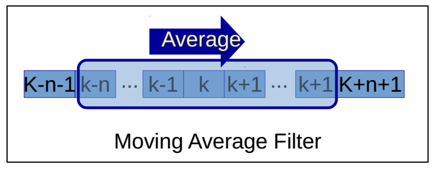
A moving average filter with window size equal to 5 was considered for smoothing the measurement uncertainties and allowing for signal restoration. Figure 3 shows a schematic representation of the signal filtering process.

Figure 3.
Simplified representation of the moving average filter.
The filtered time series were normalized in relation to their mean and standard deviation to obtain the network patterns. This procedure is important to ensure that the different orders of magnitude of the variables do not negatively affect the performance of the network. Normalization was performed according to Equation (10).
where , and represent, respectively, the measured value at time k, the mean and the standard deviation of time series x. is the normalized value of .
The ESN training consists on the determination of the weights of the readout output layer (). This was performed with the Ridge Regression (Equation (11)).
The represents the matrix with the output variables. The input weight matrix () was randomly generated with the Gaussian distribution (N(0,1)). was randomly initiated and adjusted by the scaling factor. The time series obtained through the gas lift well simulations were used to train the networks. The Echo State metaparameters (spectral radius, leak rate, regularization parameter and input scaling) were searched using the Particle Swarm Optimization (PSO) [39] method. Other parameters, like the size of the reservoir, were arbitrary chosen.
4.3. Network Evaluation
To evaluate the designed network generalization capacity, new time series were generated through simulations performed with the Rojas Soares et al. [36] model (validation sets). The idea was to evaluate the network performance for a database generated with a model with a different level of detail and considering different operating conditions, in order to evaluate the transportability of the proposed ESN architecture to a more complex situation, as it usually occurs in real applications.
The network ability was evaluated by comparing the simulated patterns and the predicted data using two criteria: the and the Coefficient of determination (). is the ratio between the standard deviation of the prediction error and the standard deviation of the original set of data. The closer it is to zero, the more accurate the estimation is. According to Cunha et al. [40], values below 0.2 can be considered good. indicates the model ability of explain the observed values and the closer it is to 1, the better the estimation performance is.
The influence of training sets size on the network capacity was also evaluated. Bigger and smaller time series were considered, as generated with the Ribeiro’s model [35], and new networks were designed and evaluated with the Rojas Soares et al. [36] validation sets.
Finally, for the last analysis, only 1 day of operation was considered. New training sets were generated through simulations performed with the Ribeiro’s model [35], considering different contents of dynamic information, and the designed networks were evaluated with the validation sets for predictions in horizons ranging from 1 to 30 time steps.
5. Results
The stationary and dynamic profiles predicted with the Ribeiro [35] and Rojas Soares et al. [36] models were obtained in order to evaluate the system behavior. Section 5.1 and Section 5.2 show the obtained results. Finally, Section 5.3 shows results obtained with the designed ESN.
The considered operational conditions for all Ribeiro’ model [35] simulations were the same ones described by Peixoto et al. [41], while simulations performed with the Rojas Soares et al. model [36] were the same described by Jahanshahi et al. [32]. The well and reservoir parameters used in all simulations are shown in Table 2.

Table 2.
Well/Reservoir parameters used in simulations.
It can be observed that the well/reservoir parameters used for simulations performed with each model were quite different. This difference provides means for evaluating the generalization capacity of the network for wells with very different characteristics.
5.1. Ribeiro’S Model
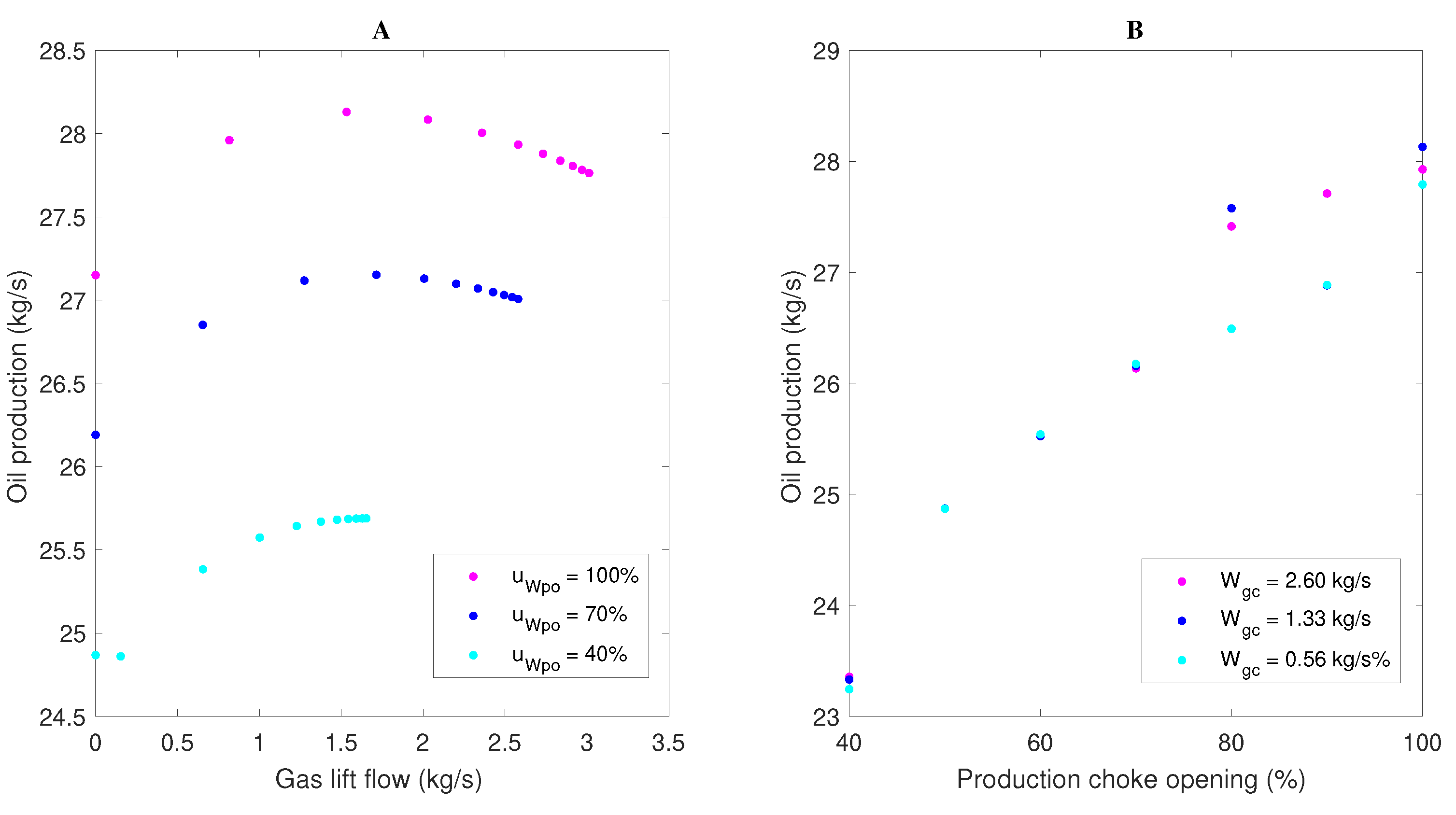
The behavior of the oil production flow (), considering three levels for the openings of the production choke valve () and gás-lift choke valve () in a range from 0 to 1, was characterized first. Figure 4A shows the results in terms of gas lift flow, because the curve of versus describes a characteristic profile for the system. The oil production flow behavior for changes of the opening of the production choke valve in a range from 0 to 1 is exhibited in Figure 4B. Three levels of gas lift flow () were considered.
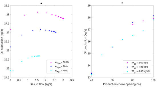
Figure 4.
Steady state profile of : changes in (A) gas lift flow; and (B) production choke valve opening—Ribeiro’s model.
Figure 4A represents a typical gas lift performance curve. It can be noticed that, at first, the oil production flow increases with the gas lift flow and seems to level off before reaching the peak. However, after a certain limit, any increase on the injection flow gradually decreases the production flow. This is because the reduction in hydrostatic pressure is no longer able to compensate the friction loss induced by the injection flow. This behavior, in principle ascending and then decreasing, indicates that the process presents a static gain signal inversion and a maximum point for the oil production. Table 3 shows the maximum value of and the corresponding value of , around which the inversion of gain signal occurs, for each analyzed opening value of the production choke valve. It can be observed in Figure 4B that, for each value of , an increase in valve opening leads to an increase in oil production flow. The maximum production flow was obtained for a gas lift flow around 1.53 kg.

Table 3.
Maximum values of and at the gain signal inversion region.
To evaluate the process dynamic behavior, the transfer functions that relate oil production flow to gas lift injection and opening of the production choke valve were determined considering the operational conditions near to the ones that lead to the high oil production. Table 4 show zeros, poles and gain obtained for each transfer function.

Table 4.
Poles, zeros and gain of system transfer functions—Ribeiro’s model.
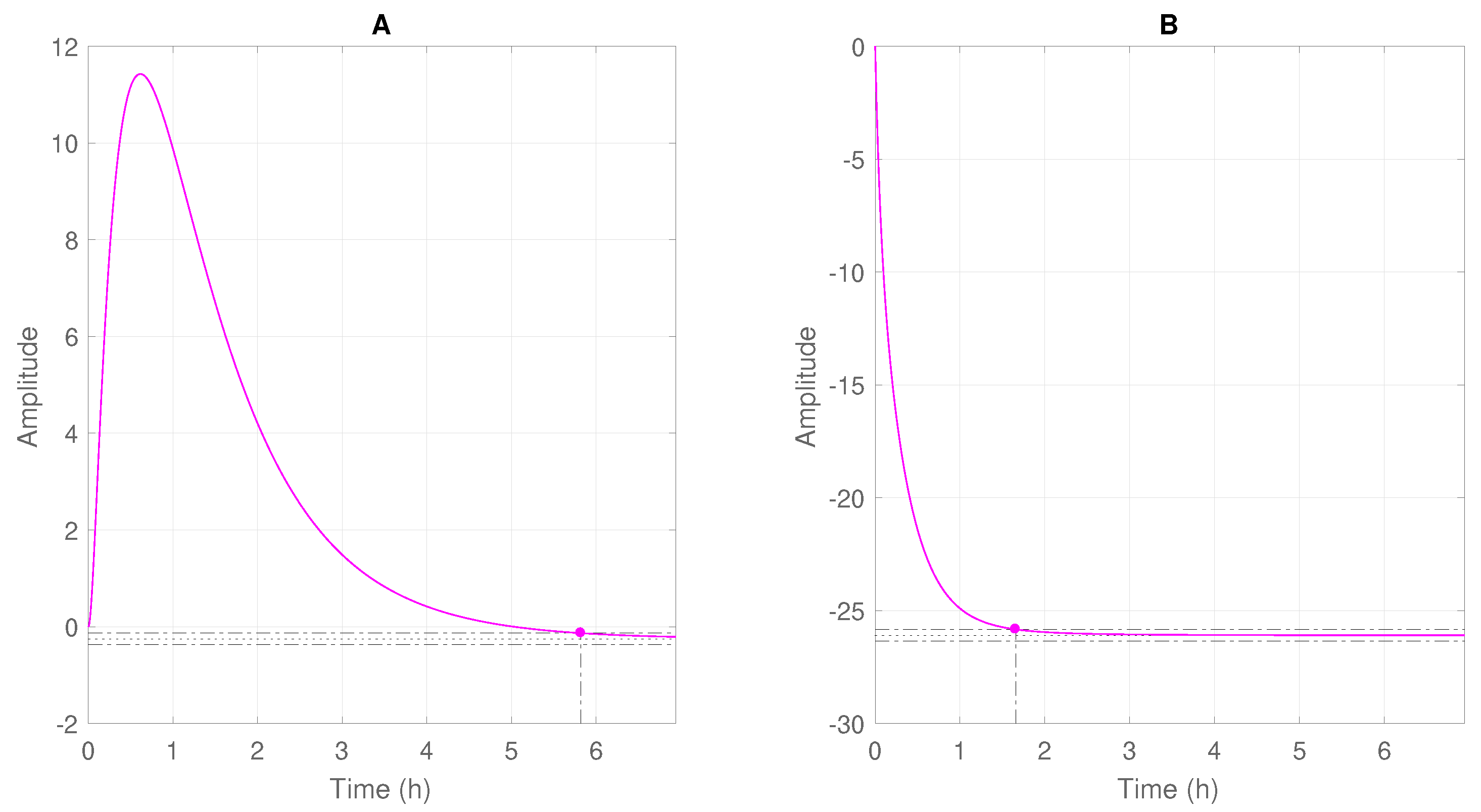
The negative poles of the system indicate, at the evaluated nominal condition, a stable behavior. The positive zero of the transfer function relating and indicates the inverse response. Figure 5 shows the obtained profiles after introduction of step disturbances in the gás lift injection rates and in the opening values of the production choke valve. The settling time, considering 1% error band, is highlighted.
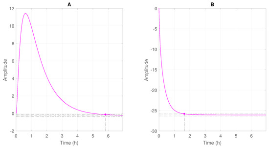
Figure 5.
Step response profiles of after changing the (A) gas lift injection (); and (B) production choke opening ().
It is worth mentioning that the analysis was performed in terms of deviation variables. As already indicated by the zeros of the transfer functions, inverse response was only observed for the case shown in Figure 5A. It can be seen initially the increase of the produced oil flow and then its stabilization at a lower stationary value after about 5.82 h. In Figure 5B it can be seen that the oil production maintained a single trend, stabilizing after 1.66 h. In both cases no dead time was noticed.
The long stabilization times indicate that the system presents slow dynamics. Then, for the dynamic simulations of the process and generation of the databases that were used for the ESN design, a sampling time of 10% of the stabilization time of the faster variable was considered.
5.2. Rojas Soares’ Model
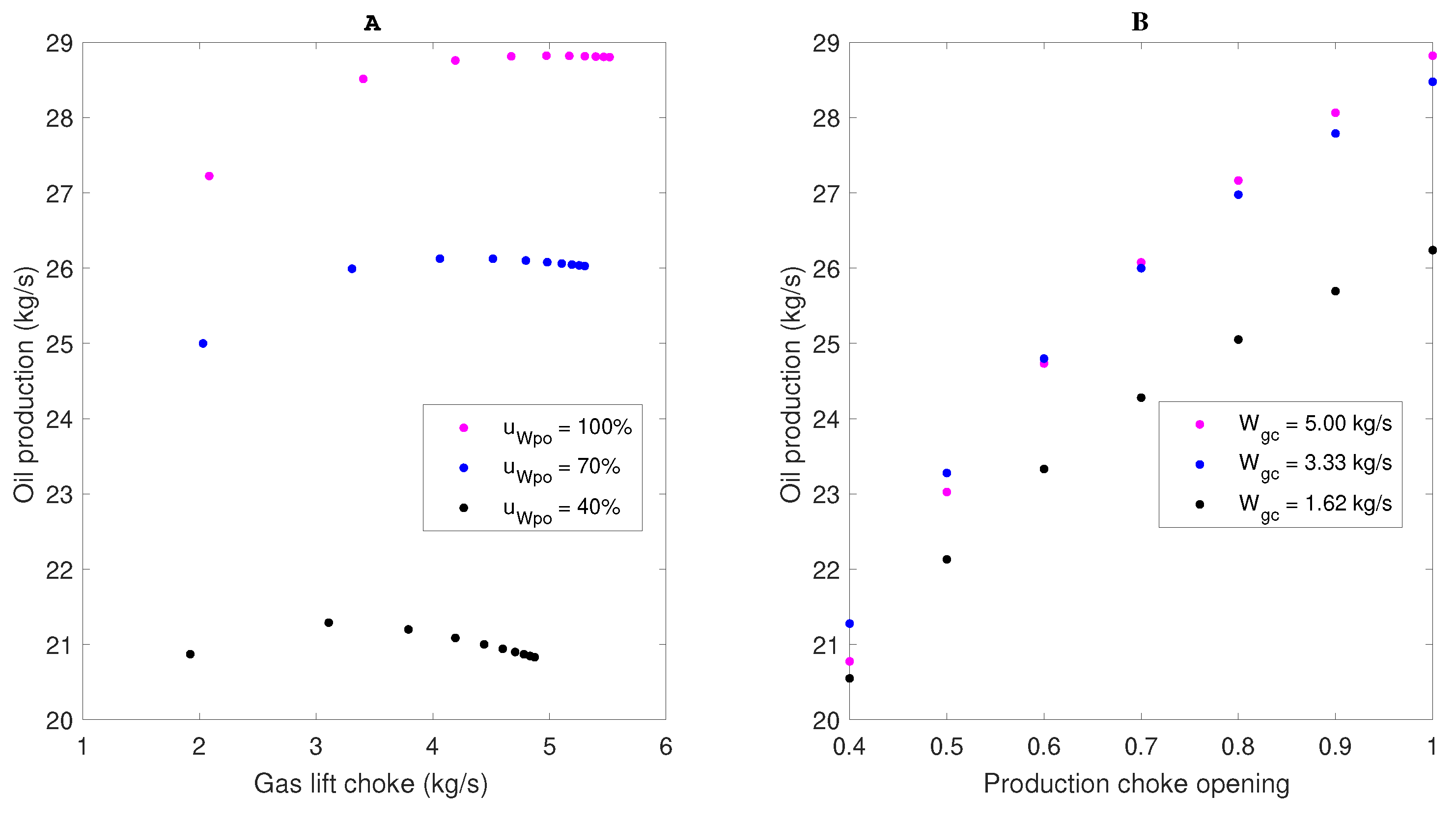
The behavior of the oil production flow (), considering the same three levels of previously considered and in a range from 0 to 1, was obtained. Figure 6A shows the results in terms of gas lift flow. The oil production flow behavior for changes in in a range from 0 to 1 is exhibited in Figure 6B. Three levels of gas lift flow were considered.
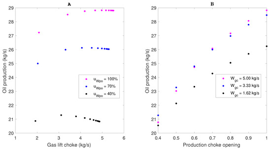
Figure 6.
Steady state profile of : changes in (A) gas lift flow; and (B) production choke valve opening—Rojas Soares et al. model [36].
The behavior of in both tests was consistent with previous results. In Figure 6A the gain signal inversion can be observed, which, in the case of the Rojas Soares et al. model, is less evident for higher opening values of the production choke valve. This indicates that, in this case, hydrostatic effects are more predominant than the effects of friction loss in the well. In Figure 6B it is possible to see that, differently from results obtained with the Ribeiro’s model, for changes in the higher was obtained with the higher level.
Then, the transfer functions that relate to and were determined for purposes of dynamic analysis. Table 5 show zeros, poles and gain obtained for each transfer function.

Table 5.
Poles, zeros and gain of system transfer functions—Roja Soares’ model.
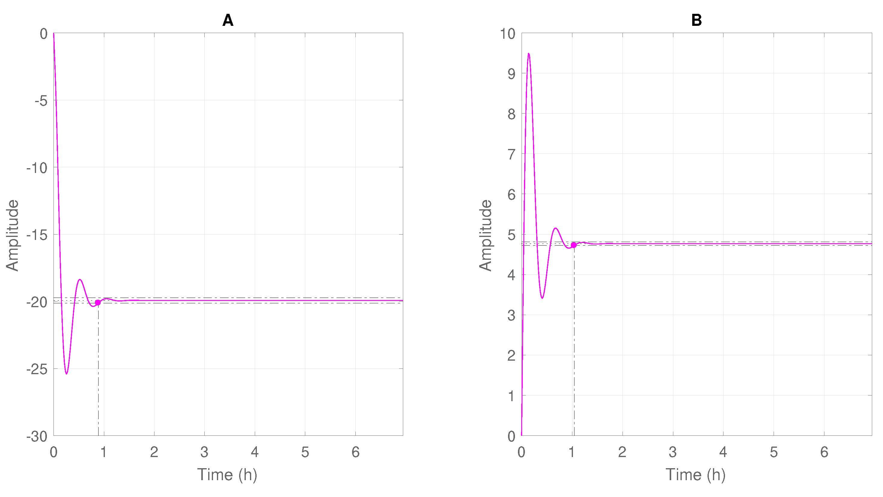
Poles and Zeros of the system exhibit negative real part, which indicates a stable behavior and a direct response, without any inverse response. Significant differences can be observed between simulation results provided by the Ribeiro’s and Rojas Soares et al. models, which is not surprising because of the significant differences among the analyzed operation conditions. Figure 7 shows dynamic profiles obtained after introduction of step disturbances in the gás lift injection rates and in the opening values of the production choke valve. The settling time, considering 1% error band, was shown.

Figure 7.
Steady state profile of —Rojas Soares et al. model.
The overshoot observed in both cases could already be expected, since the system exhibits complex conjugated poles. The poles and zeros of the system lie in the left half plane of the s plane. This characteristic is observed in the step response, since the observed profiles exhibited neither an inverse response nor an unstable behavior, stabilizing faster than the Ribeiro model.
The stabilization time of the variable with the fastest dynamics was equal to 0.887 h. It is worth noting that not only this stabilization time was distinct, but the profiles themselves were quite different. In order to define the sampling time, 10% of the stabilization time was considered, about 5 min.
5.3. Esn Evaluation—1 Step Forward
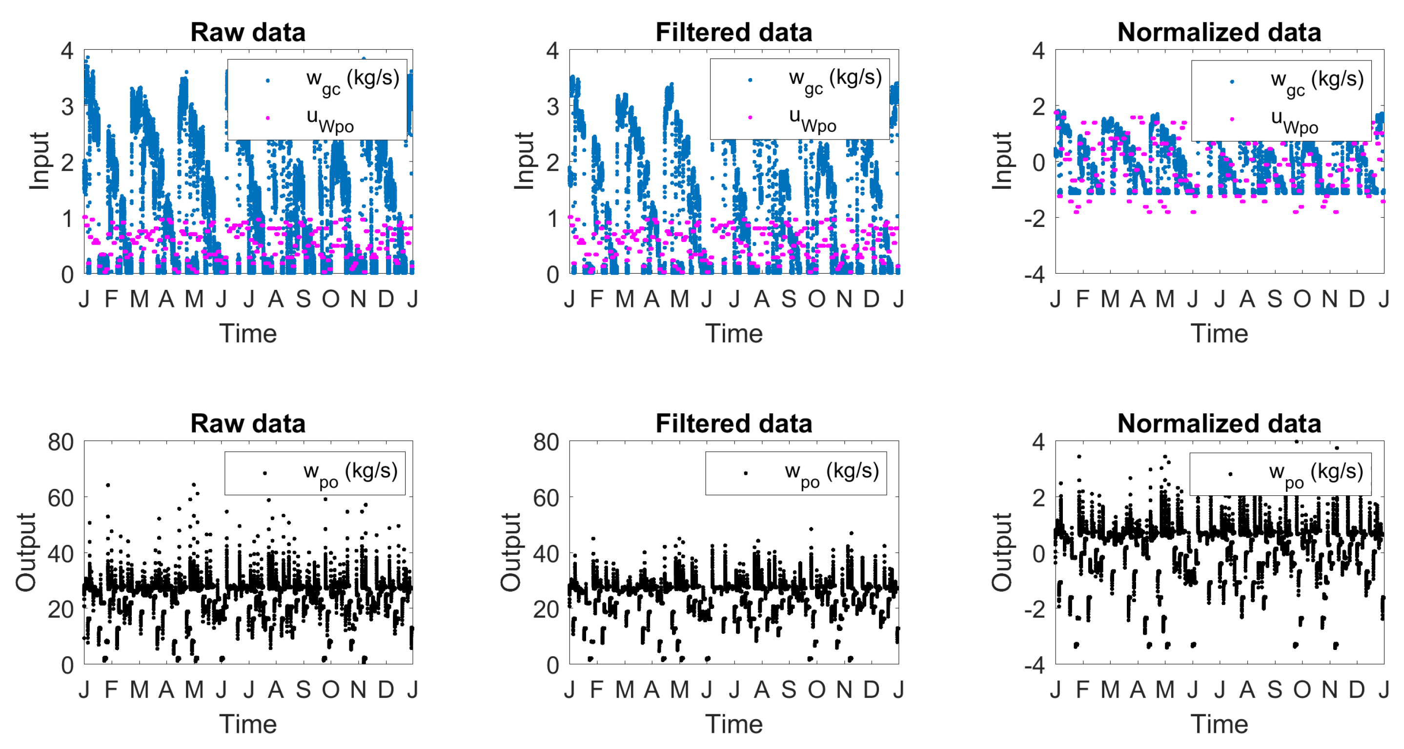
Due to the slow dynamics, shown in the previous analysis, the Ribeiro’s model was simulated considering a sampling time of 10 min. This value corresponds to approximately 1/10 of the process stabilization time. Figure 8 shows the obtained raw, filtered and normalized data for operation of 360 days.

Figure 8.
One year of the gas lift well operation.
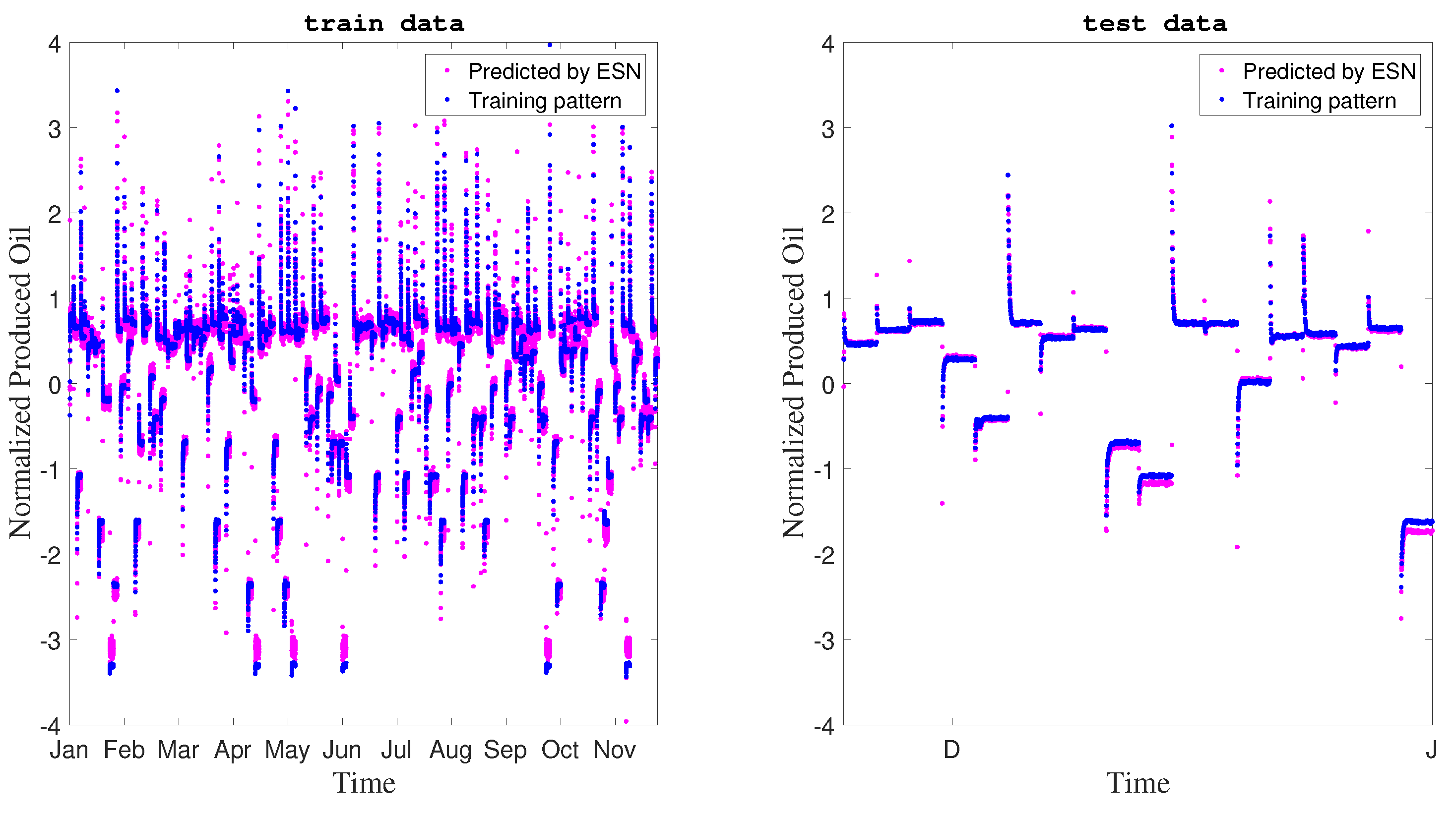
90% of the normalized data were used for Echo State Network training and 10% were used for validation tests. Figure 9 and Table 6 show the behavior obtained.
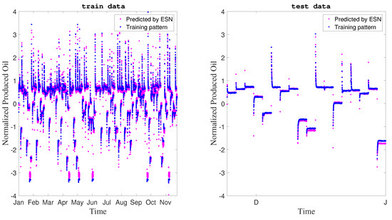
Figure 9.
Network training and test.

Table 6.
Performance Indices for training and test.
According to the and the coefficient of determination for training and test steps, the designed network presented an excellent performance. However its generalization capacity still needs to be evaluated. It is always necessary to ensure that there is a good balance between accuracy of the prediction and generalization of the model. Otherwise one can obtain into overfitting, when the network cannot predict beyond the dataset with which was designed.
Then, as a validation step, the Rojas Soares et al. [36] model was used to perform simulations, generating new data sets for network evaluation. Sampling times of 5 min were used, again considering 1/10 of the system stabilization time, shown in the previous section. Several changes were considered in the input variables, with different magnitudes and frequencies of occurrence. In addition, 10% (relative to the nominal condition) uncertainty was considered as measurement noise.
To use the network, the patterns obtained by simulation with the Rojas Soares et al. [36] model were normalized based on the characteristics of the network training set (mean and standard deviation). Table 7 summarizes the validation results, using different time series, obtained in terms of and .

Table 7.
Performance Indices for validation with the worst performance highlighted.
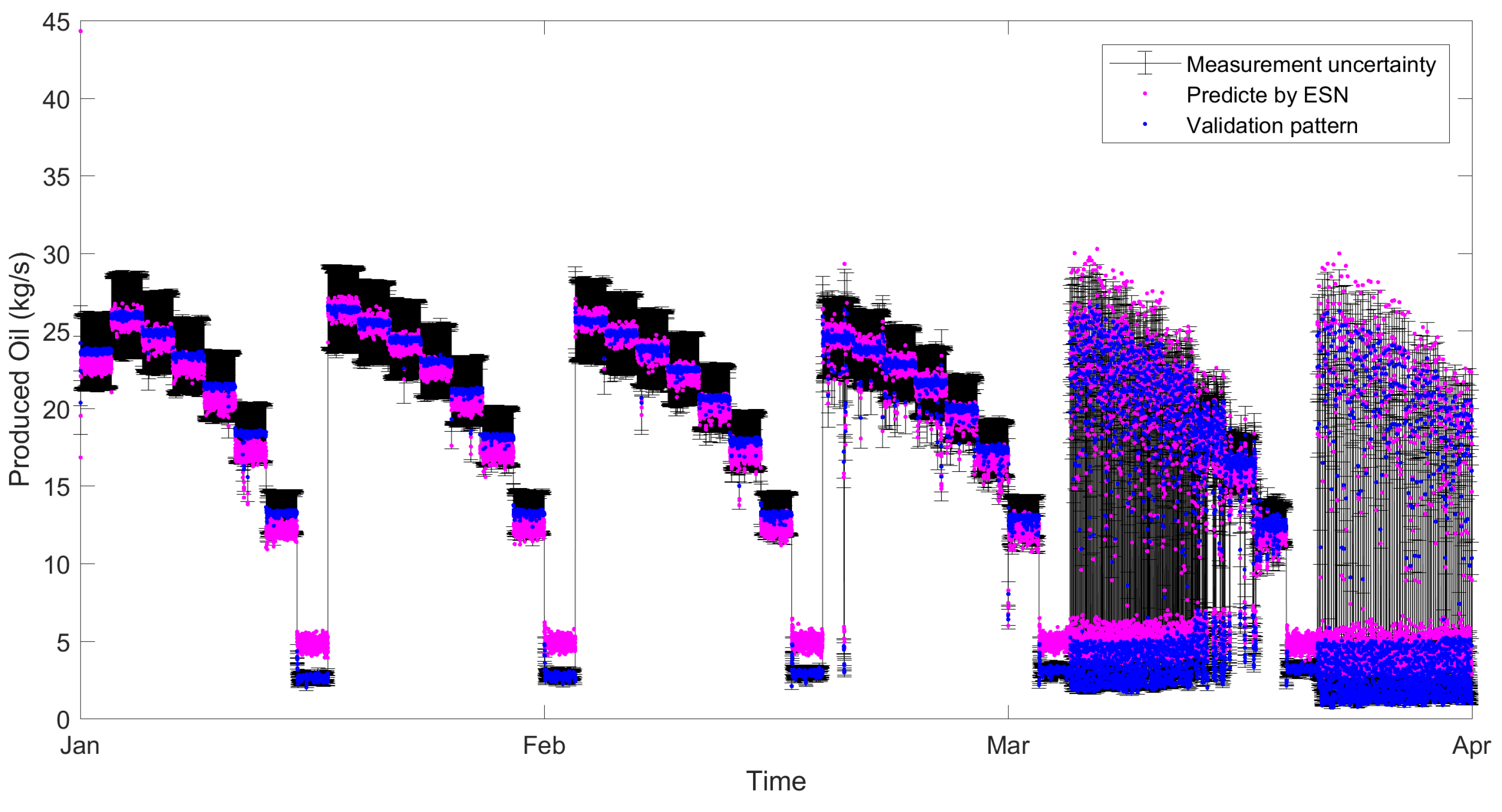
The is a measure of the prediction error dispersion level in relation to the pattern set. The obtained values, around 0.2, along with the above 0.9, indicate the good performance of the network, even in face of different operational changes and model mismatch. The worst performance, highlighted in Table 7, was evaluated and illustrated in Figure 10. Figure 10 exhibits the time series behavior with error bars and the network prediction.
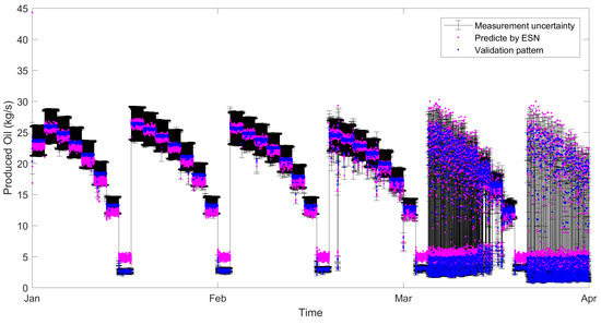
Figure 10.
Validation of the 360-day network considering the data set of 3 months.
It was observed that, even in the worst case, the values predicted by the network, were located within the measurement uncertainty range of the process, indicating that they are in the same likelihood region. Values outside this range were found in unstable operating regions.
5.4. Esn Evaluation—Time Horizon Prediction
Until now, all analysis concerned time series predictions with one step forward. Although the neural network shows an excellent performance, for use as an internal model in a predictive control strategy it is also important to evaluate its predictive ability over a future time horizon, whose measured values (pattern) are not available. In this case the network inputs at the last known instant were retained, although corrupted by a small noise, and the future outputs were calculated . Prediction horizons ranging from to and the same 6 time series used for prediction 1 step forward were then considered. Table 8 shows the obtained results.

Table 8.
Performance Index for time horizon prediction with the worst performance highlighted.
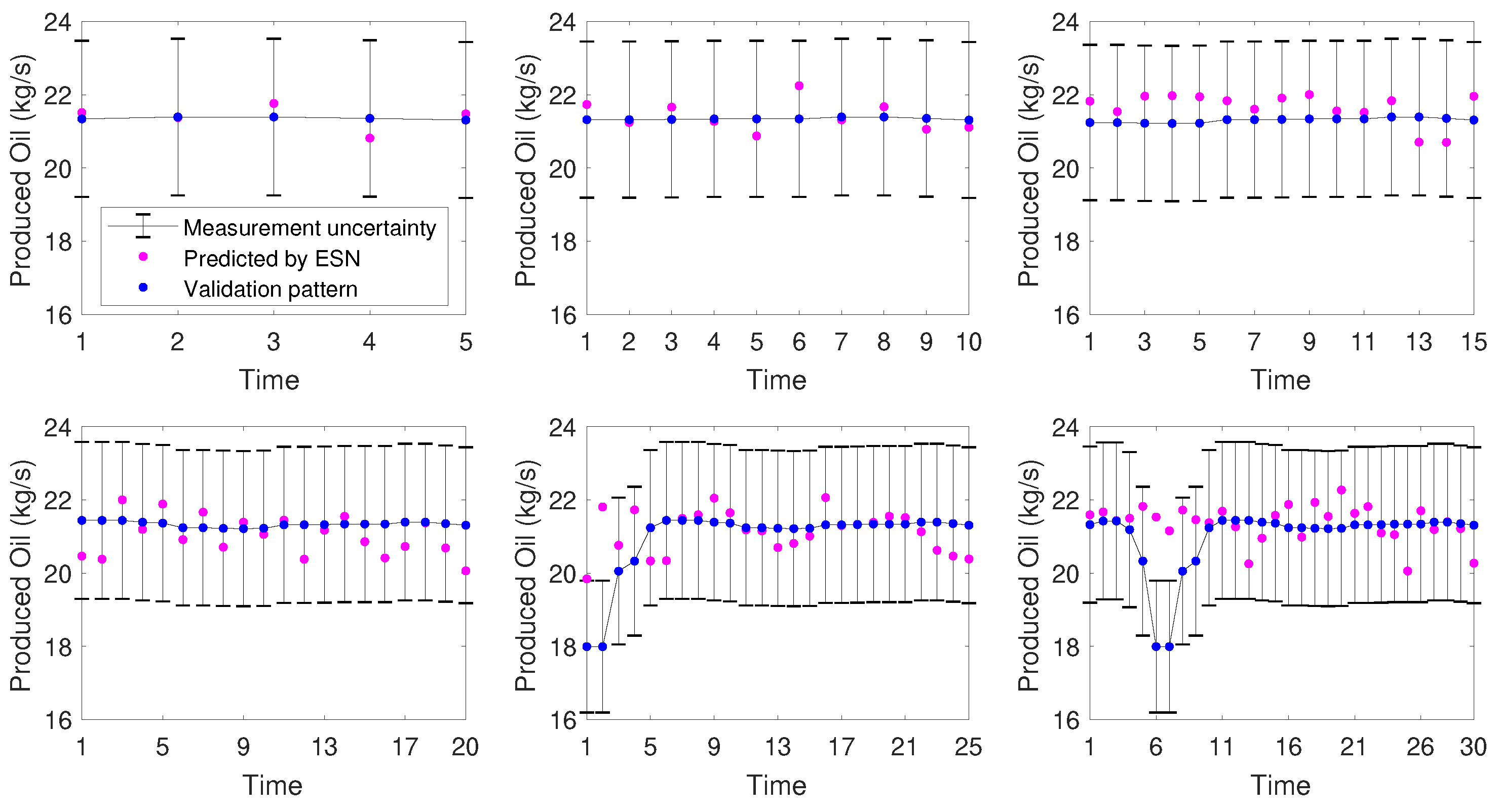
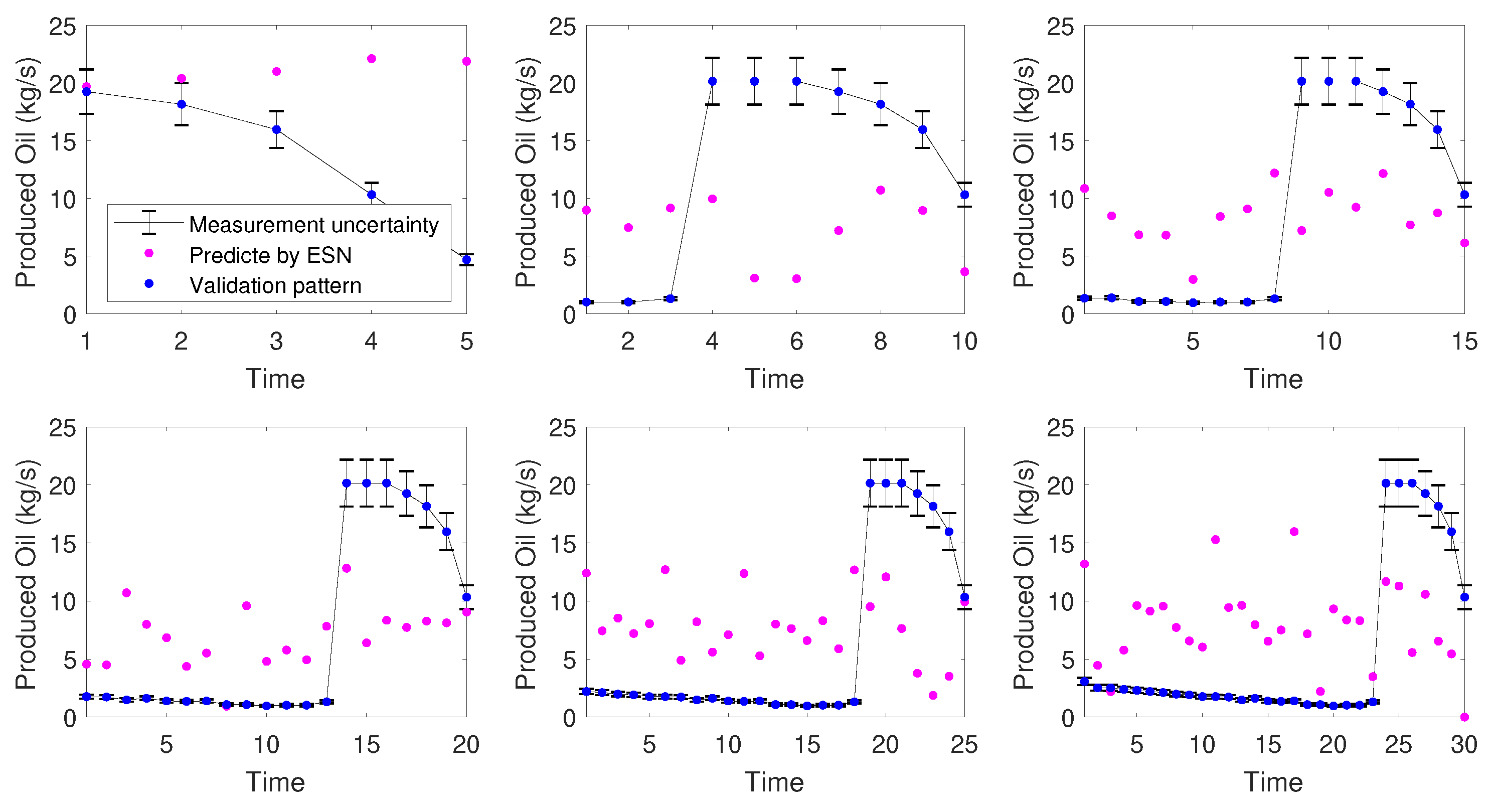
It was observed that even with the increase of the prediction horizon, there was no severe degeneration of the network prediction capacity. This indicates, once again, good performance, making it a promising tool for process control, especially when the phenomenological model of the process is not available. Again the worst performance was highlighted in Table 8. Figure 11 and Figure 12 show the behavior obtained for the 6-month time series and the 3-month time series. respectively.
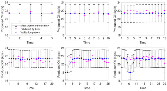
Figure 11.
Prediction in a time horizon—6 months time series.
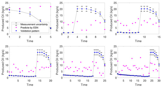
Figure 12.
Prediction in a time horizon—3 months time series.
It was observed that for the 3-month time series, which at the end points included a change in operational point, the ESN could not predict satisfactorily the process behavior in the considered time horizon. Probably because, as there is no feedback of information between the process and the network, the ESN would not be able to anticipate a change. Considering the closed control loop, the next time measurement information would arrive indicating the operational change, and then the network would be upgraded. This poor behavior was not reflected in the performance indices, since the calculation takes into account the prediction of the whole time series, and this undesired behavior was only observed in the prediction of future points, as shown in Figure 10. As for the prediction of future horizon considering the 6-month time series, the behavior of the network was very good, failing only at the point where there was significant operational fluctuation.
5.5. Esn Evaluation—Influence of Training Set Size
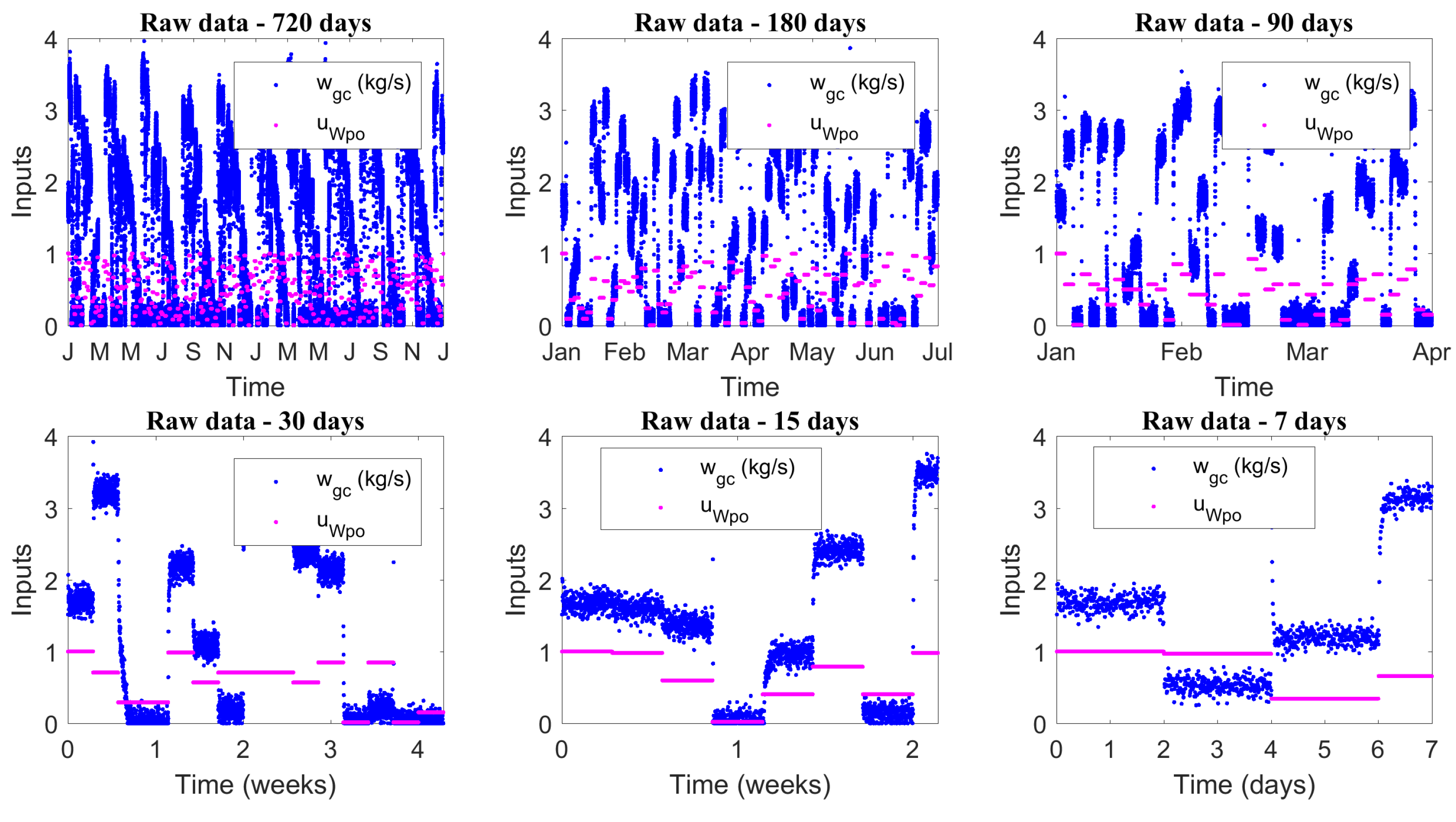
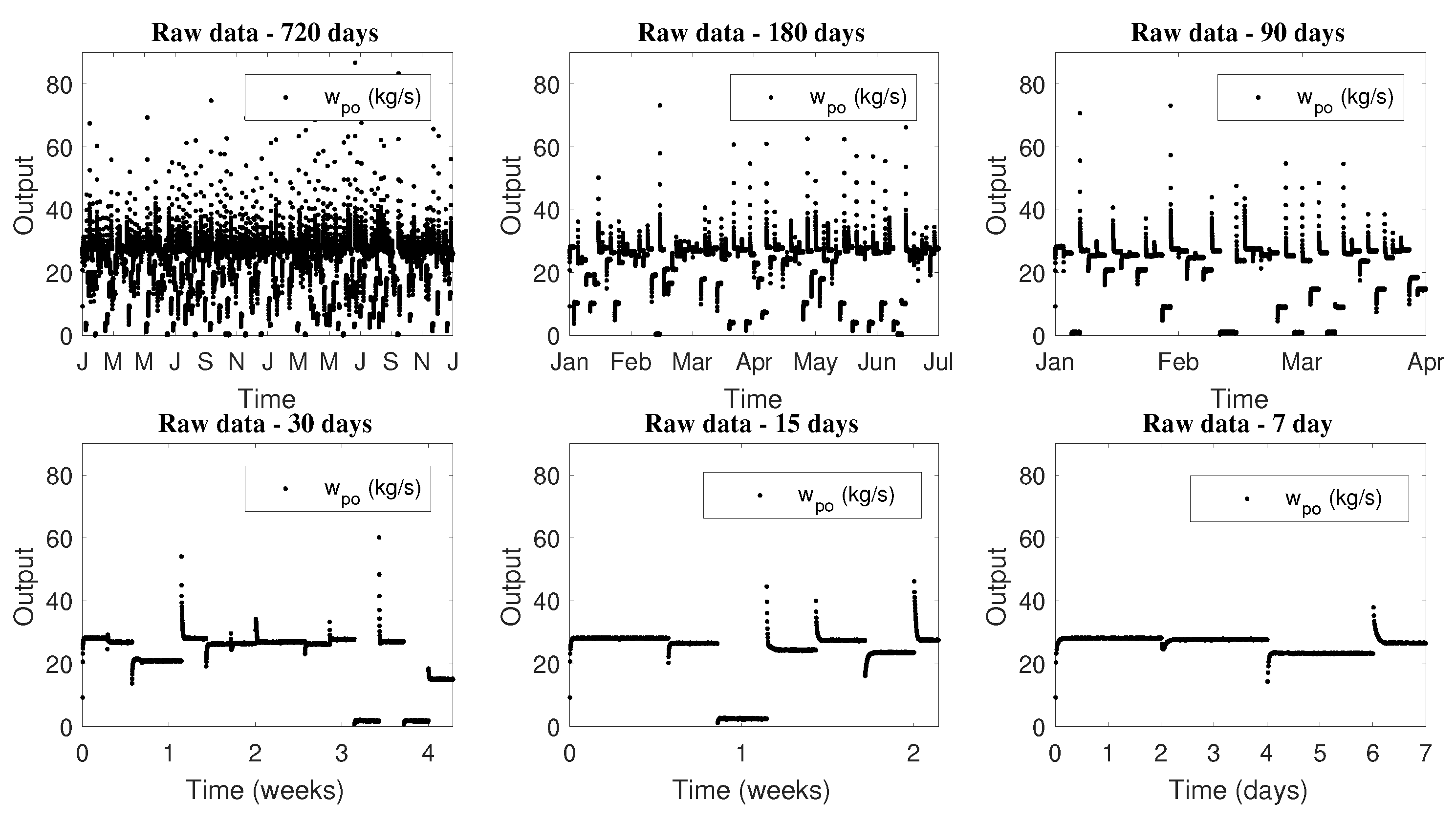
Another important aspect that is interesting to analyze is the influence of the training set size on the network prediction capacity. So, new time series were generated with the Ribeiro’ model [35] and new ESN were designed. Figure 13 and Figure 14 show operation inputs and outputs time series profiles, respectively.
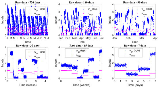
Figure 13.
Raw data time serie profiles—Inputs.

Figure 14.
Raw data time serie profiles—Output.
For training and testing of the networks the raw data were filtered and normalized. The ESN metaparameters were kept constant to exclusively evaluate the effect of training set size on the network performance. Table 9 presents the training and test results, in terms of performance index, of the new designed ESNs. In this representation, each neural network is identified by the size of the dataset used during its training.

Table 9.
Performance index for training and test of new networks.
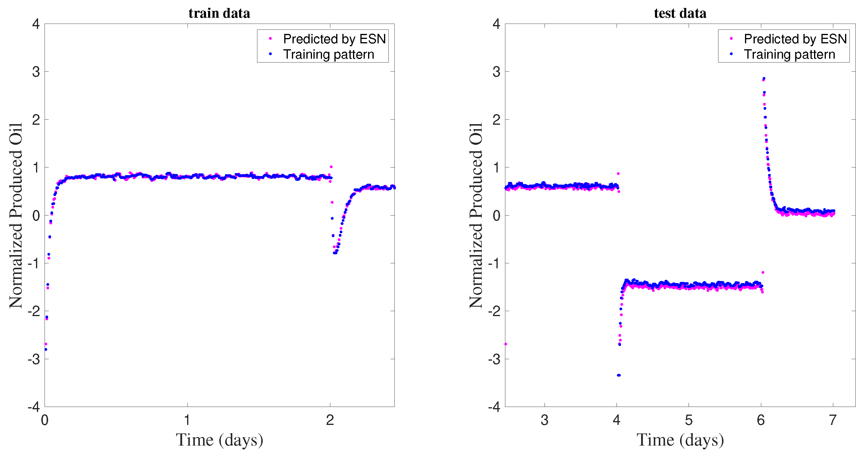
Since the echo state networks design is based on linear regression, considering larger datasets, such as 720 days, did not lead to computational problems such as memory failure and high processing time. The new networks seem to perform well, according to the determination coefficients and of the training and test steps. Figure 15 confirms this by displaying the training and test results for the network that presented the worst performance indices during training. The obtained profiles again indicate the good predictability of the network for one step forward.
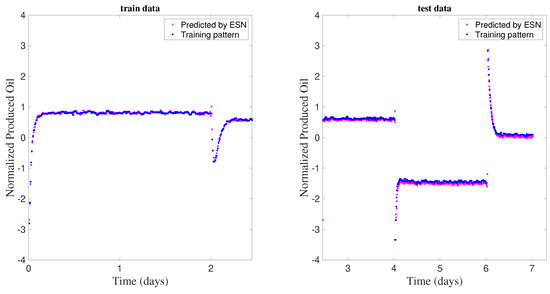
Figure 15.
Training and testing of the network designed with the 7-day time series.
These results reaffirm the good ability of echo state networks for time series predictions. However, to ensure that the ESNs presented a good generalization capacity, the same 6 time series, generated by the Rojas Soares et al. [36] model and used for evaluation of trained ESN with a 360-days set, were again considered as a validation step. Table 10 shows the results obtained, in terms of and , for prediction horizons ranging from 1 to 30.

Table 10.
Performance Indices for time horizon prediction—validation.
The trained network with 720-day data set was the one that presented the best results for all 6 validation sets. The trained networks with intermediate dataset sizes (180, 90 and 30 days) presented similar performance, but the best network was that one trained with the 90 days set. The network trained with the 7-day dataset, although exhibiting an apparent good behavior, failed during validation steps. This can indicate overfitting, as the network was not able to generalize for different conditions, or indicate that the dynamic information contained in the training set was not sufficient for the network to learn the behavior of the process. Thus, the tests for larger prediction horizons (from 5 to 30) were not performed, as indicated in Table 10.
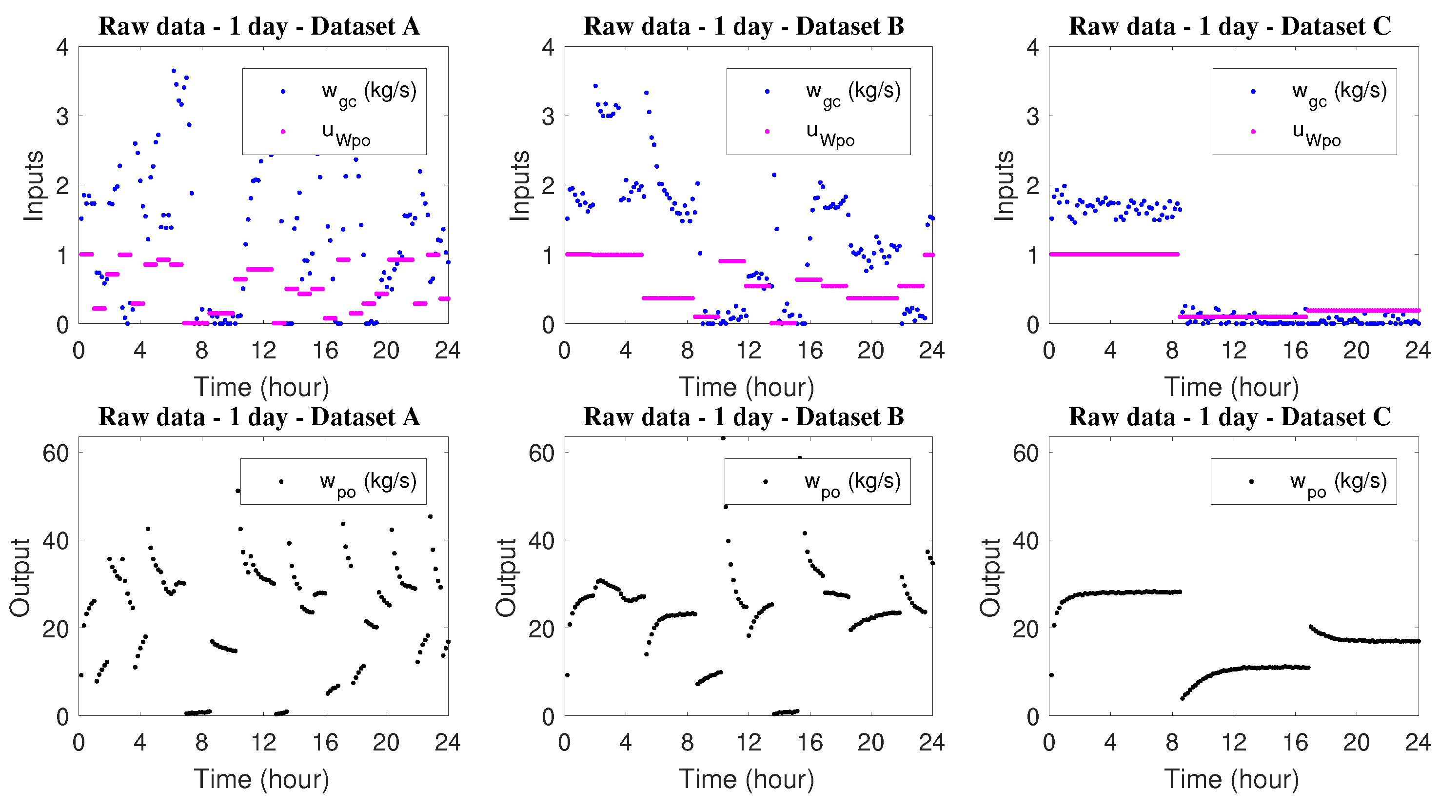
To evaluate the influence of the dynamics content in the training set, new networks were designed considering three datasets of 1 single day with different contents of dynamic information. Figure 16 shows the raw data profile used for training the networks.
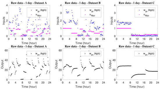
Figure 16.
Raw data time serie profiles.
The raw data was filtered and normalized for network training. Table 11 and Figure 17 show the results for both networks.

Table 11.
Performance Indices for training and test—one day of operation.
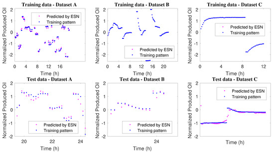
Figure 17.
Training and test profiles.
As the sampling time considered for simulations performed with the Ribeiro model was equal 10 min, 1 day of operation represents only 144 measurements. This extremely low volume of data strongly influences the performance of data-based methods such as neural networks. This is reflected in lower performance indices and poorer predicted profiles for the test steps. With little information it is much harder to achieve good generalization ability. In order to evaluate this issue, the 6 validation sets obtained from the Rojas Soares et al. simulations were was considered again. Table 12 shows the behaviors obtained for all networks.

Table 12.
Performance Indices for validation—dynamical content evaluation.
Among the three considered networks, the one with intermediate dynamic information content was the only one with performance that was sufficient to justify its use with longer prediction horizons. However, the performance indices indicate that the neural model did not present good precision for estimation of the process behavior. The other two ESN were unsuccessful during the validation stage. This was already expected due to the poor performance indices and training and test profiles shown in Table 12. Again, one possible explanation is related to overfitting. However, the dataset reported to the network was probably not sufficient for learning. Although dataset A, which has the highest content of dynamic information, is rich in operational conditions, the volume of information was still small. Thus, in fact, the size of the training set exerts enormous influence on the behavior of the network, and cannot be compensated only with a higher content of dynamic information. This aspect of ANN training has also been analyzed by others in other situations.
6. Conclusions
Echo State Networks (ESN) were used to represent the operation of gas-lift oil wells, using data generated by two distinct models. The ESN was able to predict the process behavior successfully, even for longer time horizons, indicating the stable behavior, and showing good potential for applications in predictive control. In particular, ESNs generated with a simple model were able to represent the data collected with a more rigorous model and using different parameters, indicating that the characteristics and architecture of the ESNs can be transportable, which is of fundamental importance for real implementations of the model and use in predictive controllers.
Author Contributions
As the main author of the article, A.C.S.R.D. participated in all the steps of the research that produced the results it reports, that includes: literature review, problem definition, computational implementation and simulations and analysis of the results. She also led the writing and revision steps. F.R.S. participated mostly in the activities related to the development of algoriths of the neural network and its computational implementation. J.J., J.C.P. and M.B.d.S.J. supervised the research, consolidated its results and participated in the elaboration of the manuscript itself.
Funding
This work was funded by Project “ Modeling and Control Strategies with Applications in Offshore Oil and Gas Production”, UTF-2017-CAPES-SIU/10036.
Conflicts of Interest
The authors declare no conflict of interest.
References
- Hou, Z.S.; Wang, Z. From model-based control to data-driven control: Survey, classification and perspective. Inf. Sci. 2013, 235, 3–35. [Google Scholar] [CrossRef]
- Reznik, L.; Ghanayem, O.; Bourmistrov, A. PID plus fuzzy controller structures as a design base for industrial applications. Eng. Appl. Artif. Intell. 2000, 13, 419–430. [Google Scholar] [CrossRef]
- Isaksson, A.J.; Harjunkoski, I.; Sand, G. The impact of digitalization on the future of control and operations. Comput. Chem. Eng. 2017. [Google Scholar] [CrossRef]
- Cao, Y.; Huang, J.; Ding, G.; Wang, Y. Design of Nonlinear Predictive Control for Pneumatic Muscle Actuator Based on Echo State Gaussian Process. IFAC-PapersOnLine 2017, 50, 1952–1957. [Google Scholar] [CrossRef]
- Camacho, E.; Bordons, C. Nonlinear model predictive control: An introductory review. Lect. Notes Control Inf. Sci. 2007, 358, 1–16. [Google Scholar] [CrossRef]
- Forbes, M.G.; Patwardhan, R.S.; Hamadah, H.; Gopaluni, R.B. Model predictive controlin industry: Challenges and opportunities. IFAC-PapersOnLine 2015, 28, 531–538. [Google Scholar] [CrossRef]
- Hou, Z.S.; Xu, J.X. On Data-driven Control Theory: The State of the Art and Perspective. Acta Autom. Sin. 2009, 35, 650–667. [Google Scholar] [CrossRef]
- Oussous, A.; Benjelloun, F.Z.; Ait Lahcen, A.; Belfkih, S. Big Data technologies: A survey. J. King Saud Univ. Comput. Inf. Sci. 2018, 30, 431–448. [Google Scholar] [CrossRef]
- Chen, M.; Mao, S.; Zhang, Y.; Leung, V.C. Big Data; SpringerBriefs in Computer Science; Springer: Cham, Switzerland, 2014; Volume 15, pp. 283–285. [Google Scholar] [CrossRef]
- Amaral, F. Introdução à Ciencia de Dados: Mineração de Dados e Big Data; Alta Books Editora: Rio de Janeiro, Brasil, 2016. [Google Scholar]
- Antonelo, E.A.; Camponogara, E.; Foss, B. Echo State Networks for data-driven downhole pressure estimation in gas-lift oil wells. Neural Netw. 2017, 85, 106–117. [Google Scholar] [CrossRef]
- Yin, S.; Li, X.; Gao, H.; Kaynak, O. Data-based techniques focused on modern industry: An overview. IEEE Trans. Ind. Electron. 2015, 62, 657–667. [Google Scholar] [CrossRef]
- Lee, J.H.; Shin, J.; Realff, M.J. Machine learning: Overview of the recent progresses and implications for the process systems engineering field. Comput. Chem. Eng. 2017. [Google Scholar] [CrossRef]
- Samarasinghe, S. Neural Networks for Applied Sciences and Engineering—From Fundamentals to Complex Pattern Recognition; Auerbach Publications: New York, NY, USA, 2006; p. 560. [Google Scholar]
- Haykin, S. Neural Networks: A Comprehensive Foundation; Prentice Hall PTR: Upper Saddle River, NJ, USA, 1994. [Google Scholar]
- Jaeger, H. The “echo state” approach to analysing and training recurrent neural networks-with an erratum note. Bonn Ger. Ger. Natl. Res. Cent. Inf. Technol. GMD Tech. Rep. 2001, 148, 13. [Google Scholar]
- De Canete, J.F.; del Saz-Orozco, P.; Gonzalez, S.; Garcia-Moral, I. Dual composition control and soft estimation for a pilot distillation column using a neurogenetic design. Comput. Chem. Eng. 2012, 40, 157–170. [Google Scholar] [CrossRef]
- Cracknell, M.J.; Reading, A.M. Geological mapping using remote sensing data: A comparison of five machine learning algorithms, their response to variations in the spatial distribution of training data and the use of explicit spatial information. Comput. Geosci. 2014, 63, 22–33. [Google Scholar] [CrossRef]
- Bas, E.; Uslu, V.R.; Egrioglu, E. Robust learning algorithm for multiplicative neuron model artificial neural networks. Expert Syst. Appl. 2016, 56, 80–88. [Google Scholar] [CrossRef]
- Zhang, M.; Liu, X.; Zhang, Z. A soft sensor for industrial melt index prediction based on evolutionary extreme learning machine. Chin. J. Chem. Eng. 2016, 24, 1013–1019. [Google Scholar] [CrossRef]
- Sant Anna, H.R.; Barreto, A.G.; Tavares, F.W.; de Souza, M.B. Machine learning model and optimization of a PSA unit for methane-nitrogen separation. Comput. Chem. Eng. 2017, 104, 377–391. [Google Scholar] [CrossRef]
- Danilo, P.M.; Chambers, J.A. Recurrent Neural Network for Prediction; John Wiley & Sons, Ltd.: Hoboken, NJ, USA, 2001; Volume 4. [Google Scholar]
- Lukoševičius, M. A Practical Guide to Applying Echo State Networks; Springer: Berlin/Heidelberg, Germany, 2012; pp. 659–686. [Google Scholar] [CrossRef]
- Doya, K. Bifurcations in the learning of recurrent neural networks. In Proceedings of the 1992 IEEE International Symposium on Circuits and Systems, San Diego, CA, USA, 10–13 May 1992; Volume 6, pp. 2777–2780. [Google Scholar] [CrossRef]
- Huang, J.; Qian, J.; Liu, L.; Wang, Y.; Xiong, C.; Ri, S. Echo state network based predictive control with particle swarm optimization for pneumatic muscle actuator. J. Frankl. Inst. 2016, 353, 2761–2782. [Google Scholar] [CrossRef]
- Jordanou, J.P.; Antonelo, E.A.; Camponogara, E.; de Aguiar, S.; Aurelio, M. Recurrent Neural Network based control of an Oil Well. In Proceedings of the Brazilian Symposium on Intelligent Automation, Porto Alegre, Brazil, 1–4 October 2017. [Google Scholar]
- Jordanou, J.P.; Camponogara, E.; Antonelo, E.A.; Aguiar, M.A.S. Nonlinear Model Predictive Control of an Oil Well with Echo State Networks. IFAC-PapersOnLine 2018, 51, 13–18. [Google Scholar] [CrossRef]
- Plucenio, A.; Ganzaroli, C.A.; Pagano, D.J. Stabilizing gas-lift well dynamics with free operating point. In Proceedings of the 2012 IFAC Workshop on Automatic Control in Offshore Oil and Gas Production, Trondheim, Norway, 31 May–1 June 2012; Volume 1, pp. 95–100. [Google Scholar] [CrossRef]
- Hu, B. Characterizing Gas-lift Instabilities. Ph.D. Thesis, Norwegian University of Science and Technology, öTrondheim, Norway, 2004. [Google Scholar]
- Eikrem, G.; Imsland, L.; Foss, B. Stabilization of gas-lifted wells based on state estimation. IFAC Proc. Vol. 2004, 37, 323–328. [Google Scholar] [CrossRef]
- Aamo, O.M.; Eikrem, G.O.; Siahaan, H.B.; Foss, B.A. Observer design for multiphase flow in vertical pipes with gas-lift—-Theory and experiments. J. Process Control 2005, 15, 247–257. [Google Scholar] [CrossRef]
- Jahanshahi, E.; Skogestad, S.; Hansen, H. Control Structure Design for Stabilizing Unstable Gas-Lift Oil Wells; IFAC: Geneva, Switzerland, 2012; Volume 8, pp. 93–100. [Google Scholar] [CrossRef]
- Grimstad, B.; Foss, B. A nonlinear, adaptive observer for gas-lift wells operating under slowly varying reservoir pressure. IFAC Proc. Vol. 2014, 47, 2824–2829. [Google Scholar] [CrossRef]
- Eikrem, G.O.; Aamo, O.M.; Foss, B.A. On instability in gas lift wells and schemes for stabilization by automatic control. SPE Prod. Oper. 2008, 23, 268–279. [Google Scholar] [CrossRef]
- Ribeiro, C.H.P. Controle Preditivo Multivariável com Requisitos de Qualidade em Plataformas de Produção de Petróleo. Master’s Thesis, COPPE/UFRJ, Rio de Janeiro, Brasil, 2012. [Google Scholar]
- Rojas Soares, F.D.; Souza, M.B., Jr.; Secchi, A. Development of an MPC for stabilization and optimization of a gas lift oil well. In Annual Colloquium of Chemical Engineering; Instituto Alberto Luiz Coimbra de Pós-Graduação e Pesquisa de Engenharia, Universidade Federal do Rio de Janeiro: Rio de Janeiro, Brasil.
- Peng, D.Y.; Robinson, D.B. A new two-constant equation of state. Ind. Eng. Chem. Fundam. 1976, 15, 59–64. [Google Scholar] [CrossRef]
- fsolve Matlab—MathWorks Description. Available online: https://www.mathworks.com/help/optim/ug/fsolve.html (accessed on 21 March 2019).
- Schwaab, M.; Biscaia, E.C., Jr.; Monteiro, J.L.; Pinto, J.C. Nonlinear parameter estimation through particle swarm optimization. Chem. Eng. Sci. 2008, 63, 1542–1552. [Google Scholar] [CrossRef]
- Cunha, F.; Souza, M.; O M Folly, R. Melt index flow and xylene solubles content virtual sensor applied to industrial production of polypropylene. In Proceedings of the XVIII Congresso Brasileiro de Engenharia Química, Foz do Iguacu, Brasil, 19–20 September 2010. [Google Scholar]
- Jacoud, A.; Diego, P.; Pereira-dias, D.; Secchi, A.R.; Secchi, A.R. Modelling and Extremum Seeking Control of Gas Lifted Oil Wells. IFAC-PapersOnLine 2015, 48, 21–26. [Google Scholar] [CrossRef]
© 2019 by the authors. Licensee MDPI, Basel, Switzerland. This article is an open access article distributed under the terms and conditions of the Creative Commons Attribution (CC BY) license (http://creativecommons.org/licenses/by/4.0/).

