Article

Control Charts for Monitoring Process Capability Index Using Median Absolute Deviation for Some Popular Distributions

1
Department of Statistics, Faculty of Science, King Abdulaziz University, Jeddah 21551, Saudi Arabia
2
Department of Statistics, the University of Dodoma, Dodoma, PO. Box: 259, Tanzania
3
Department of Statistics and Computer Science, University of Veterinary & Animal Sciences, Lahore 54000, Pakistan
4
Department of Industrial and Management Engineering, Pohang University of Science and Technology, Pohang 790-784, Korea
*
Author to whom correspondence should be addressed.
Processes 2019, 7(5), 287; https://doi.org/10.3390/pr7050287
Submission received: 4 February 2019 / Revised: 7 May 2019 / Accepted: 13 May 2019 / Published: 15 May 2019

Abstract

:
A control chart monitoring the process capability index (PCI) using median absolute deviation (MAD) is proposed to analyze the industrial process performance. Extensive simulation studies were carried out to evaluate the performance of MAD-based PCI control charts under the low, moderate, and high asymmetric conditions when the process characteristic follows Weibull, log-normal, and gamma distributions. The performance of the proposed control charts was evaluated based on the average run lengths. The practical implementation of the proposed charts was also illustrated with industrial data.

1. Introduction

A control chart is an important tool of statistical process control for monitoring the process mean, dispersion or both to enhance customer trust and the quality of the production process. The combined study of the process means, process dispersion, and process target can be numerically examined by the application of the commonly known technique of process capability indices. Several process capability indices have been developed in the quality control literature, but the most commonly applied indices are C p ,   C p k ,   C p m   and   C p m k [1,2,3,4]. Many other process capability indices have been derived from these four basic indices [5]. These four indices can be derived from a single formula developed by [6] using two non-negative parameters. Any production process can be best monitored and evaluated using these indices with the assumption that it follows a normal distribution [7], which in many cases is doubtful because either the distribution of interested quality characteristic is unknown or it does not follow a normal distribution [8]. Further, the estimation of the mean and variance becomes suspicious because of the unexpected variation in the error of the estimated parameters [9,10]. Hosseinifard et al. [11] claimed that the study of process capability indices for non-normal data may lead to erroneous results. Therefore, the study of non-normal data has long been a great challenge for researchers [7,8,9,10,12,13].
Clements [14] proposed a quantile approach for the parameter estimation of non-normal data, which is the most commonly employed approach among many others for this purpose. It has been shown in the literature that the use of process capability indices for a heavily skewed distribution provides misleading estimates [15]. The researchers [16,17,18,19,20] claimed that the use of median absolute deviation (MAD) is the best alternative to the standard deviation for non-normal data. The use of MAD in the quality control literature has been studied by many researchers, including the authors of [17,20].
The performance evaluation of the proposed control chart can be studied using the average run length (ARL), which is defined as the average number of samples before the process indicates the out-of-control signal. The ARL when the process is in control is denoted by ARL0 [21]. It is considered that the value of ARL0 should be larger, as it indicates the process is in the form of in control. The expected number of samples from the out-of-control process should be smaller, as it indicates the out-of-control process as quickly as possible, which is denoted by ARL1. References [21,22] used a martingale approach for the derivation of the ARL formula for the normal as well as for the non-normal distributions. A numerical integration approach was applied by [23] to evaluate the performance of the proposed control chart. Several basic and commonly used methods for the calculation of the ARL for the exponentially weighted moving average (EWMA) and cumulative sum (CUSUM) charts were reviewed by [24]. Many researchers of quality control charts have used the ARL for the performance evaluation of the proposed charts, including [22,25,26,27,28,29,30,31,32,33,34].
The objective of this paper is to develop a monitoring scheme for the production process using the process capability index with MAD. The rest of the paper is organized as follows: Process capability indices using MAD is explained in Section 2. In Section 3, the design of MAD control charts for non-normal distributions is developed. An example of the practical implementation of the proposed scheme is included in Section 4. The conclusion is given in the last section.

2. Process Capability Indices (PCIs) Using Median Absolute Deviation

A process capability index (PCI) is a unit-free quantitative measure that compares the behavior of manufactured process characteristics. Process capability indices have been used extensively in many fields for the purpose of process measurement and enhancement. More notably, using process capability indices, quality engineers specify what is going on in the production process at ground level with a single measurement value and the necessary steps for product improvement. The process capability index, C p k , defined by [1], is given as:
C p k = d | μ m | 3 σ ,
where   d = ( U S L L S L ) / 2 , m = ( U S L + L S L ) / 2 ,   μ and σ 2 represent the mean and variance of the process, respectively. Here, USL is upper specification limit and LSL lower specification limit.
This PCI can be interpreted accurately when the process follows a normal distribution. For non-normal data, the median absolute deviation (MAD) is a good robust estimator of the standard deviation ( σ ) in case of a non-normal distribution [16,17,18,19,20].
Suppose that the sample median (SM) is computed from a random sample ( x 1 , x 2 , , x n ) . Then, MAD from the SM (MMAD) is defined as [18,35,36]:
M M A D = b × M A D ,
where M A D = m e d i a n { | x i M | } .
The value of constant b in (2) is used to make the parameter of interest a consistent estimator. In the case of an unbiased estimator of σ , we need to set b = 1.4826 if a random sample is taken from a normal distribution. For a non-normal distribution, this value changes to b = 1/Q(0.75), where Q(0.75) is the 0.75 quantile of the underlying distribution. In case of normality, 1/Q(0.75) = 1.4826 [37]. Thus, the unbiased estimator of σ is:
σ ^ = 1.4826 ( M A D ) .
The PCI based on MAD is obtained using an unbiased estimator of σ in Equation (1), and it is given as:
C ^ p k = m i n { U S L M 3 σ ^ , M L S L 3 σ ^ }     = m i n { U S L M 4.45 M A D , M L S L 4.45 M A D } ,
where M is median. According to Aslam et al. (2017), for non-normal distributions based on waiting times, which gives a positive value, the LSL should be considered as 0. Meanwhile, Park [38] suggested, for obtaining the LSL and USL values for skewed distributions, using the procedure L S L = F ( 0.005 ) and U S L = F ( 0.995 ) , where F ( . ) is a cumulative distribution function of corresponding distribution.

3. Design of MAD Control Charts for Non-Normal Distributions

In this section, we study the MAD control chart for process capability C ^ p k , given in Equation (3) for non-normal distributions like Weibull, gamma, and log-normal distributions, which is sorted as low, moderate, and high asymmetric level skewness; for more details, see Kashif et al. [39].
Let X represent a random variable taken from Weibull distribution with shape parameter γ and scale parameter β . Then, the probability density function (p.d.f) is written as:
f ( x ) = γ β   ( x β ) γ 1 e ( x β ) γ ;   x 0 .
If X follows a log-normal distribution with mean μ and scale parameter σ , then p.d.f is written as:
f ( x ) = 1 x σ 2 π exp ( 1 2 ( ln ( x ) μ σ ) ) ; x > 0 .
If X follows a gamma distribution with scale β and shape parameter λ , then p.d.f is given by:
f ( x ) = 1 β λ Γ λ x λ 1 exp ( x / β ) ; x 0 .
The proposed MAD control chart plots the values of C ^ p k for each subgroup of size n, and the process is said to be out of control if the plotted statistic C ^ p k is outside the upper control limit (UCL) and lower control limit (LCL). The proposed MAD control chart when the process characteristic follows Weibull, log-normal, and gamma distributions can be obtained with the following steps:
Step 1: Select a random sample of size n from the production process and measure the quality variable X.
Step 2: Compute the sample median M and the MAD from Equation (2). Here, b = 1/Q(0.75), where Q(0.75) is the 0.75 quantile of the underlying distribution.
Step 3: Compute the C ^ p k using the following formula:
C ^ p k = m i n { U S L M 4.45 M A D , M L S L 4.45 M A D } ,
where M is the sample median of the sample data.
Step 3: State the process capability index as out of control if C ^ p k LCL .
Let C ¯ p k and S C p k be the mean and standard deviation, respectively, for C ^ p k , which should be obtained from subgroup data when a process is in control. The LCL for the proposed chart is in the following form:
LCL = C ¯ p k k S C p k ,
where k is a control chart coefficient to be obtained.
The performance of the proposed control chart can be studied using average run length (ARL). There are two types of ARLs available in the literature to study the performance of control charts, that is, in-control ARL (ARL0) and out-of-control ARL (ARL1). ARL0 is the average number of samples that triggers a control chart signals, when the process is in control. ARL0 should be as large as possible, since the process is in control. ARL1 is the average number of samples until a control chart signals when the process is out of control. The performance of the control chart is assessed by ARL1, with smaller values of ARL1 indicating the supremacy of the chart.
The ARL for the in-control process (denoted by ARL0) is obtained by:
A R L 0 = 1 P o u t 0 .
When the process is in control at θ = θ 0 , P o u t 0 can be computed as follows:
P o u t 0 = P ( C ^ p k < L C L | θ = θ 0 ) .
Assume that there is a change in the scale parameter ( θ ) of the Weibull, log-normal, and gamma distributions when the shape parameter remains unchanged. The scale parameter ( θ ) of the Weibull, log-normal, and gamma distributions is assumed to be shifted to θ 1 = θ 0 c , where c is shift-constant. When the process is shifted from θ 0   to   θ 1 , the probability of the proposed process stated as in control is given as follows:
P o u t 1 = P ( C ^ p k < L C L | θ = θ 1 )
.
The ARL for the out-of-control process is denoted by ARL1 and given by:
A R L 1 = 1 P o u t 1 .
The performance of the proposed control chart is studied using Monte Carlo simulation. The simulation is applied to obtain the values of ARL0, ARL1, and control chart coefficient k. Suppose that r 0 represents the specified in-control ARL0. The summary of an algorithm is as follows:
Step 1: Generate each subgroup random sample of size n from Weibull or log-normal or gamma distribution with the specified in-control process. Generate such N subgroups.
Step2: Compute C ^ p k for each subgroup and then compute mean and standard deviation from N subgroups.
Step 3: Fix the in-control ARL, say, r 0 .
Step 4: Determine the value of control chart coefficient k such that ARL 0 r 0 .
Step 5: Obtain the out-of-control ARLs for various shifts values c.
Table 1, Table 2, Table 3, Table 4, Table 5, Table 6, Table 7, Table 8, Table 9, Table 10, Table 11, Table 12, Table 13, Table 14, Table 15, Table 16, Table 17 and Table 18 present specified r 0 = 370, 300, 250, and 200; n = 25, 50 for three non-normal distributions. The following are observations noticed from the tables for the proposed control chart.
1. The ARL value decreases as n increases when other parameters are fixed.
2. The ARL value increases as the shape parameter increases for three distributions when other parameters are fixed.
3. The ARL value decreases as c increases when other parameters are fixed.
4. Between the nature of the distributions, the ARL values increase from low to high asymmetry estimators. The same trend is observed for the three non-normal distributions considered in this study.

4. Example

In this section, we give the presentation of the proposed control chart using simulated data. The following procedure is used for generating data and constructing the control charts:
Step 1: Choose a random sample of size n.
Step 2: Generate Weibull/gamma/log-normal random variables X of size n with different parametric combinations.
Step 3: Obtain the chart statistic C ^ p k .
Step 4: Repeat steps 1 to 3 until the desired number of sample groups (m) is attained.
Step 5: Construct the control limits described in Section 3.
Step 6: Plot all statistics C ^ p k against their sample groups.
Simulation Results for Weibull Distribution
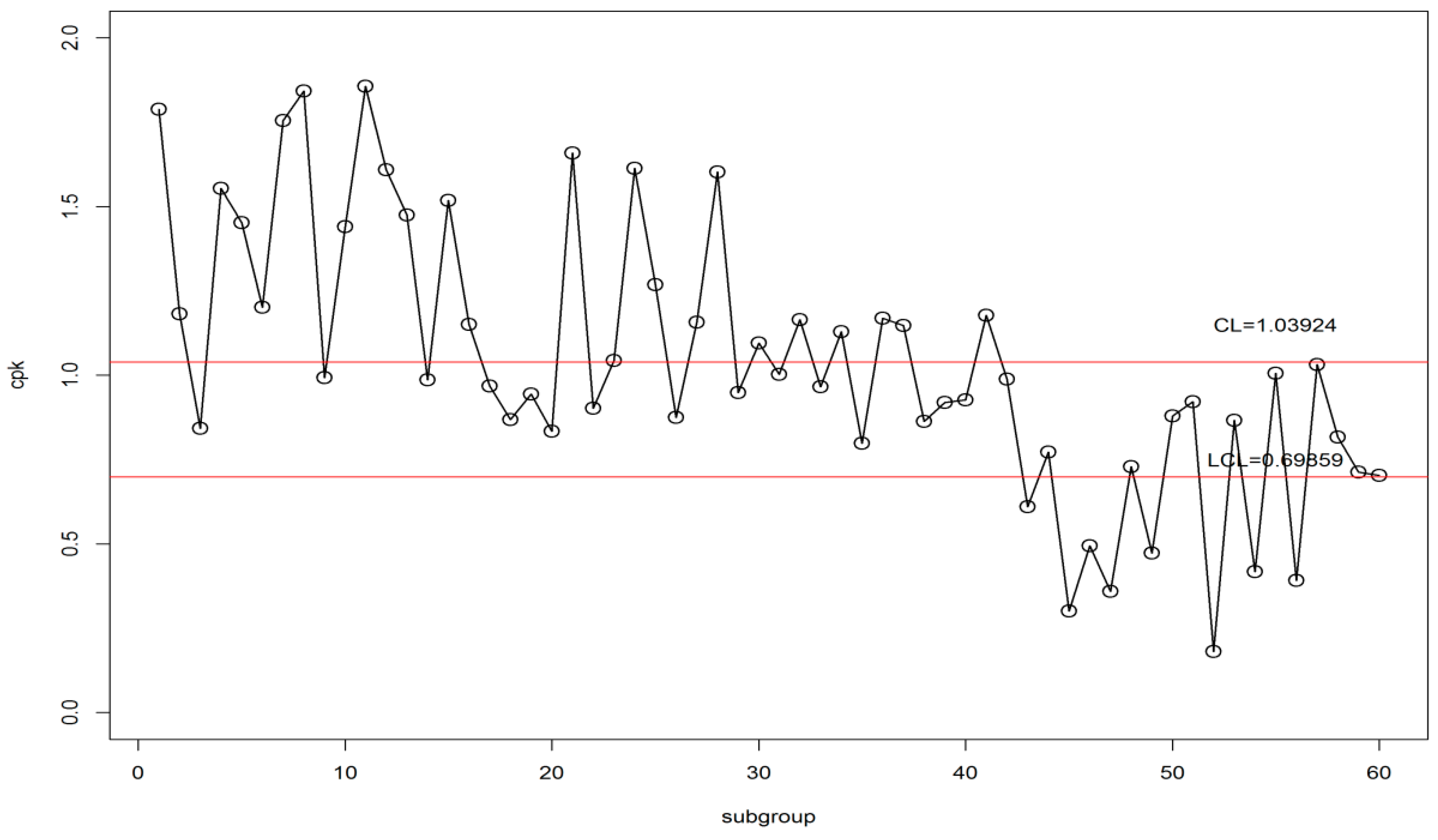
For this design, the first 30 samples of subgroup size 25 were generated from the Weibull distribution with in-control shape parameters = 1.8 and scale parameter = 2.0, and the second set of the 30 samples of subgroup size 25 is from the Weibull distribution with shape = 1.8 and scale = 1.7 (i.e., out-of-control situation having a shift of c = 0.30). In Table 3, when ARL0 at 370 and the specific in-control shape = 1.8 and scale = 2.0, we found the control chart lower limit LCL = 0.69859 for the proposed chart at n = 25 . The lists of the C ^ p k values for these 60 simulations are given below. The graphical display of the proposed control chart is presented in Figure 1.
From Figure 1, we can see that the proposed chart quickly detects the shift in the process at the 33rd sample, which is the 3rd subgroup after the true shift. Thus, we conclude that there is a downward shift in the process, indicating that the process is in an out-of-control state.
Weibull simulated C ^ p k data: 1.7886, 1.1817, 0.8427, 1.5540, 1.4526, 1.2016, 1.7546, 1.8425, 0.9932, 1.4401, 1.8570, 1.6092, 1.4756, 0.9869, 1.5183, 1.1506, 0.9684, 0.8683, 0.9448, 0.8343,1.6586, 0.9018, 1.0434, 1.6131, 1.2689, 0.8746, 1.1569, 1.6030, 0.9482, 1.0952, 1.0030, 1.1647, 0.9655, 1.1297, 0.7988, 1.1692, 1.1478, 0.8632, 0.9196, 0.9275, 1.1781, 0.9890, 0.6099, 0.7721, 0.3010, 0.4950, 0.3593, 0.7296, 0.4734, 0.8798, 0.9212, 0.1809, 0.8667, 0.4174, 1.0061, 0.3918, 1.0317, 0.8172, 0.7130, 0.7036.
Simulation Results for Gamma Distribution
In this design, the first 31 samples of subgroup size 25 were generated from the gamma distribution with in-control shape parameters = 3 and scale parameter = 0.75, and the second set of the 31 samples of subgroup size 25 is from the gamma distribution with shape = 3 and scale = 0.65 (i.e., out-of-control situation having a shift of c = 0.10). In Table 9, when ARL0 at 370 and the specific in-control shape = 3 and scale = 0.75, we found LCL = 0.86988 for the proposed chart at n = 25 . The lists of the C ^ p k values for these 62 simulations are given below. The graphical display of the proposed control chart is presented in Figure 2.
From Figure 2, we can see that the proposed chart quickly detects the shift in the process at the 39th sample, which is the 7th subgroup after the true shift. Thus, we conclude that the process is in an out-of-control state.
Gamma simulated C ^ p k data: 1.4367, 2.1233, 1.4984, 0.9290, 1.4843, 1.9834, 1.9983, 2.1801, 2.1520, 2.2172, 1.5942, 1.5054, 1.7511, 2.3804, 2.0640, 2.0678,0.8804, 1.5343, 1.3319, 1.1727, 2.3253, 1.8682, 1.7044, 1.2893, 1.4973, 2.0875, 1.5482, 1.1785,1.8909, 0.9298, 0.9656, 1.6618, 1.2472, 1.3836, 0.9271, 0.9638, 1.1434, 1.0847, 0.4415, 1.0789, 0.9573, 0.4464, 0.6148, 1.3356, 1.5011, 0.9733, 1.0705, 0.8874, 1.0127, 0.7991, 0.5731, 1.0733, 1.1819, 0.3897, 0.7396, 1.1123, 1.4479, 0.9587, 0.6478, 0.8251, 0.5678, 0.7008.
Simulation Results for Log-Normal Distribution
In this design, the first 29 samples of subgroup size 25 were generated from the log-normal distribution with in-control mean = 0.5 and standard deviation = 1.00, and the second set of the 29 samples of subgroup size 25 is from the log-normal distribution with mean = 0.4 and standard deviation = 1.00 (i.e., out-of-control situation having a shift of c = 0.10). In Table 15, when ARL0 at 370 and the specific in-control mean = 0.5 and standard deviation = 1.00, we found LCL = 0.782699 for the proposed chart at n = 25 . The lists of the C ^ p k values for these 58 simulations are given below. The graphical display of the proposed control chart is presented in Figure 3.
From Figure 3, we can see that the proposed chart quickly detects the shift in the process at the 34th sample, which is the 6th subgroup after the true shift. Thus, we conclude that there is a downward shift in the process, indicating that the process is in an out-of-control state.
Log-normal simulated C ^ p k data: 0.8408, 0.9910, 0.8576, 1.8336, 1.5079, 1.7591, 1.1089, 1.3588, 0.9609, 1.4330, 1.7608, 0.8624, 0.9404, 0.8923, 1.1141, 1.1059, 1.0810, 1.0956, 1.4138, 1.7512, 1.3910, 1.0702, 0.9856, 1.1715, 1.4992, 1.5478, 1.6865, 0.8602, 0.8312, 0.9903, 1.3583, 0.9777, 0.8892, 0.7416, 1.1836, 1.2369, 0.8918, 0.7719, 0.5765, 1.8737, 0.8675, 0.7878, 0.4639, 0.9297, 0.5545, 0.4538, 0.7519, 0.9452, 1.2168, 0.9186, 0.6568, 0.7695, 0.4347, 0.3557, 0.8512, 0.8131, 0.6281, 0.9185.
Moreover, when we compared the performance between three distributions, it was noticed that gamma distribution performed well with respect to ARLs. For different samples, sizes, and shift constants considered in this study, ARL values were smaller than for the other two distributions, whereas log-normal distribution showed a very close performance to gamma distribution. Furthermore, we noticed from Figure 1, Figure 2, and Figure 3 that gamma distribution performed well as compared to Weibull and log-normal distribution.

5. Conclusions

In this article, a control chart was developed for the process capability indices C p k using median absolute deviation for non-normal distributions like Weibull, gamma, and log-normal distribution, which were classified as low, moderate, and high asymmetric levels of skewness. The control chart constants were obtained for different process parameters and average run lengths for various shift levels using a simulation technique. The article also furnished a detailed procedure for the design and extensive tables of ARL for the out-of-control process for different shifts in scale parameters. The methodology of the proposed control charts has been included in this paper using simulated data. It was observed that the proposed control chart design is effective in the quick detection of the out-of-control process. Between the nature of the distributions, ARL values increase from low to high asymmetry estimators. The same trend was observed for the three non-normal distributions considered in this study.

Author Contributions

M.A., G.S.R., A.H.A.-M., L.A., and C.-H.J. conceived and designed the experiments. M.A. and A.H.A.-M. performed the experiments. M.A. and A.H.A.-M. analyzed the data. M.A. contributed reagents/materials/analysis tools. M.A. wrote the paper.

Funding

This article was funded by the Deanship of Scientific Research (DSR) at King Abdulaziz University, Jeddah. The authors, therefore, acknowledge and thank DSR for the technical and financial support.

Acknowledgments

The authors are deeply thankful to the editor and reviewers for their valuable suggestions to improve the quality of this manuscript.

Conflicts of Interest

The authors declare no conflict of interest regarding this paper.

References

  1. Kane, V.E. Process capability indices. J. Qual. Technol. 1986, 18, 41–52. [Google Scholar] [CrossRef]
  2. Ahmad, L.; Aslam, M.; Jun, C.-H. Designing of X-bar control charts based on process capability index using repetitive sampling. Trans. Inst. Meas. Control 2014, 36, 367–374. [Google Scholar] [CrossRef]
  3. Panichkitkosolkul, W. Confidence Interval for the Process Capability Index Cp Based on the Bootstrap-t Confidence Interval for the Standard Deviation. Metodol. Zv. 2014, 11, 79–92. [Google Scholar]
  4. Zhang, J. Conditional Confidence Intervals of Process Capability Indices Following Rejection of Preliminary Tests; The University of Texas: Arlington, TX, USA, 2010. [Google Scholar]
  5. Pearn, W.; Chen, K. Estimating process capability indices for non-normal Pearsonian populations. Qual. Reliab. Eng. Int. 1995, 11, 386–388. [Google Scholar] [CrossRef]
  6. Vännman, K. A uniformed approach to capability indices. Stat. Sin. 1995, 5, 805–820. [Google Scholar]
  7. Sennaroglu, B.; Senvar, O. Performance comparison of box-cox transformation and weighted variance methods with weibull distribution. J. Aeronaut. Space Technol. 2015, 8, 49–55. [Google Scholar] [CrossRef]
  8. Piña-Monarrez, M.R.; Ortiz-Yañez, J.F.; Rodríguez-Borbón, M.I. Non-normal Capability Indices for the Weibull and Lognormal Distributions. Qual. Reliab. Eng. Int. 2015, 32, 1321–1329. [Google Scholar] [CrossRef]
  9. Senvar, O.; Kahraman, C. Type-2 fuzzy process capability indices for non-normal processes. J. Intell. Fuzzy Syst. 2014, 27, 769–781. [Google Scholar]
  10. Senvar, O.; Kahraman, C. Fuzzy Process Capability Indices Using Clements’ Method for Non-Normal Processes. J. Mult.-Valued Log. Soft Comput. 2014, 22, 95–121. [Google Scholar]
  11. Hosseinifard, Z.; Abbasi, B.; Niaki, S. Process capability estimation for leukocyte filtering process in blood service: A comparison study. IIE Trans. Healthc. Syst. Eng. 2014, 4, 167–177. [Google Scholar] [CrossRef]
  12. Leiva, V.; Marchant, C.; Saulo, H.; Aslam, M.; Rojas, F. Capability indices for Birnbaum–Saunders processes applied to electronic and food industries. J. Appl. Stat. 2014, 41, 1881–1902. [Google Scholar] [CrossRef]
  13. Senvar, O.; Sennaroglue, B. Comparing Performance of Clements, Box-Cox, Johnson Methods with Weibull Distributions for Assessing Process Capability. J. Ind. Eng. Manag. 2016, 9, 634–656. [Google Scholar] [CrossRef]
  14. Clements, J.A. Process capability calculations for non-normal distributions. Qual. Prog. 1989, 22, 95–97. [Google Scholar]
  15. Wu, C.W.; Pearn, W.L.; Chang, C.S.; Chen, H.C. Accuracy Analysis of the Percentile Method for Estimating Non-normal Manufacturing Quality. Commun. Stat. Simul. Comput. 2007, 36, 657–696. [Google Scholar] [CrossRef]
  16. Rodriguez, R.N. Recent Developments in Process Capability Analysis. J. Qual. Technol. 1992, 24, 176–187. [Google Scholar] [CrossRef]
  17. Shu, M.-H.; Hsu, B.-M.; Han, C.-P. Estimation of Industrial Process Capabilities: Some Estimators to Overcome the Obstacle of Non-normal Distributions. Available online: https://pdfs.semanticscholar.org/92c6/6a314aaf8e28a70d246241a91e9e96264fa6.pdf (accessed on 1 February 2019).
  18. Abu-Shawiesh, M.O. A simple robust control chart based on MAD. J. Math. Stat. 2008, 4, 102. [Google Scholar]
  19. Shahriari, H.; Maddahi, A.; Shokouhi, A.H. A robust dispersion control chart based on M-estimate. J. Ind. Syst. Eng. 2009, 2, 297–307. [Google Scholar]
  20. Adekeye, K.S. Process Capability Indices Based on Median Absolute Deviation. Int. J. Appl. 2013, 3, 43–48. [Google Scholar]
  21. Montgomery, D.C. Introduction to Statistical Quality Control, 6th ed.; John Wiley & Sons, Inc.: New York, NY, USA, 2009. [Google Scholar]
  22. Sukparungsee, S.; Novikov, A. On EWMA procedure for detection of a change in observation via Martingale approach. KMITL Sci. J. 2006, 6, 373–380. [Google Scholar]
  23. Phanyaem, S.; Areepong, Y.; Sukparungsee, S. Numerical Integration of Average Run Length of CUSUM Control Chart for ARMA Process. Int. J. Appl. Phys. Math. 2014, 4, 232–235. [Google Scholar] [CrossRef]
  24. ZLi, H.; Zou, C.L.; Gong, Z.; Wang, Z.J. The computation of average run length and average time to signal: An overview. J. Stat. Comput. Simul. 2014, 84, 1779–1802. [Google Scholar]
  25. Knoth, S. Accurate ARL Calculation for EWMA Control Charts Monitoring Normal Mean and Variance Simultaneously. Seq. Anal. 2007, 26, 251–263. [Google Scholar] [CrossRef]
  26. Lee, M.; Khoo, M.B. Optimal statistical design of a multivariate EWMA chart based on ARL and MRL. Commun. Stat. Simul. Comput. 2006, 35, 831–847. [Google Scholar] [CrossRef]
  27. Balamurali, S.; Aslam, M.; Ahmad, L. Determination of a New Mixed Variable Lot-Size Multiple Dependent State Sampling Plan Based on the Process Capability Index. Commun. Stat. Theory Methods 2017, 47, 615–627. [Google Scholar] [CrossRef]
  28. Aslam, M.; Rao, G.S.; Ahmad, L.; Jun, C.-H. A control chart for multivariate Poisson distribution using repetitive sampling. J. Appl. Stat. 2017, 44, 123–136. [Google Scholar] [CrossRef]
  29. Aslam, M.; Saghir, A.; Ahmad, L.; Jun, C.-H.; Hussain, J. A control chart for COM-Poisson distribution using a modified EWMA statistic. J. Stat. Comput. Simul. 2017, 87, 3491–3502. [Google Scholar] [CrossRef]
  30. Aslam, M.; Khan, N.; Ahmad, L.; Jun, C.-H.; Hussain, J. A mixed control chart using process capability index. Seq. Anal. 2017, 36, 278–289. [Google Scholar] [CrossRef]
  31. Ahmad, L.; Aslam, M.; Arif, O.H.; Jun, C.H. Dispersion Chart for Some Popular Distributions under Repetitive Sampling. J. Adv. Mech. Des. Syst. Manuf. 2016, 10. [Google Scholar] [CrossRef]
  32. Amdouni, A.; Castagliola, P.; Taleb, H.; Celano, G. Monitoring the coefficient of variation using a variable sample size control chart in short production runs. Int. J. Adv. Manuf. Technol. 2015, 81, 1–14. [Google Scholar] [CrossRef]
  33. Azam, M.; Aslam, M.; Jun, C.-H. Designing of a hybrid exponentially weighted moving average control chart using repetitive sampling. Int. J. Adv. Manuf. Technol. 2014, 77, 1927–1933. [Google Scholar] [CrossRef]
  34. Yan, A.; Liu, S.; Dong, X. Variables two stage sampling plans based on the coefficient of variation. J. Adv. Mech. Des. Syst. Manuf. 2016, 10. [Google Scholar] [CrossRef]
  35. Rousseeuw, P.J.; Croux, C. Alternatives to the median absolute deviation. J. Am. Stat. Assoc. 1993, 88, 1273–1283. [Google Scholar] [CrossRef]
  36. Haque, M.E.; Khan, J.A. Globally Robust Confidence Intervals for Location. Dhaka Univ. J. Sci. 2012, 60, 109–113. [Google Scholar] [CrossRef]
  37. Leys, C.; Ley, C.; Klein, O.; Bernard, P.; Licata, L. Detecting outliers: Do not use standard deviation around the mean, use absolute deviation around the median. J. Exp. Soc. Psychol. 2013, 49, 764–766. [Google Scholar] [CrossRef]
  38. Park, H.I. A New Definition on the Process Capability Index Based on Quantiles. Appl. Math. Sci. 2017, 11, 173–183. [Google Scholar] [CrossRef]
  39. Kashif, M.; Aslam, M.; Al-Marshadi, A.H.; Jun, C.-H. Capability Indices for Non-Normal Distribution Using Gini’s Mean Difference as Measure of Variability. IEEE Access 2016, 4, 7322–7330. [Google Scholar] [CrossRef]
Figure 1. Proposed Weibull median absolute deviation (MAD) control chart for simulated data.
Processes 07 00287 g001
Figure 2. Proposed gamma MAD control chart for simulated data.
Processes 07 00287 g002
Figure 3. Proposed log-normal MAD control chart for simulated data.
Processes 07 00287 g003
Table 1. The average run lengths (ARLs) for the proposed chart when n = 25, WD(2.8,3.5), upper specification limit (USL) = 6.3488, and lower specification limit (LSL) = 0.5280.
LCL1.45531.47551.49471.5207
cARL0 = 370ARL0 = 300ARL0 = 250ARL0 = 200
0.0370.78300.28250.18200.14
0.1223.91186.82156.87125.04
0.2136.13114.7897.3978.75
0.383.3371.6761.7251.22
0.453.1245.5339.4933.28
0.533.8929.6626.0022.11
0.622.1219.6717.4815.11
0.714.9313.4012.0710.40
0.810.179.158.367.47
0.97.266.656.125.54
1.05.294.874.554.17
Table 2. The ARLs for the proposed chart when n = 50, WD(2.8,3.5), USL = 6.3488, and LSL = 0.5280.
LCL1.71751.73641.75261.7729
cARL0 = 370ARL0 = 300ARL0 = 250ARL0 = 200
0.0370.60300.72250.33200.09
0.1187.45154.39129.15106.36
0.297.5780.8168.8858.18
0.351.8244.0538.3432.26
0.428.8825.0422.2519.33
0.517.0615.0313.4511.81
0.610.359.228.397.49
0.76.635.975.525.01
0.84.444.083.813.53
0.93.183.002.842.66
1.02.382.262.162.04
Table 3. The ARLs for the proposed chart when n = 25, WD(1.8,2.0), USL = 5.0504, and LSL = 0.1055.
LCL0.698590.707480.715290.72491
cARL0 = 370ARL0 = 300ARL0 = 250ARL0 = 200
0.0370.36300.49250.21200.39
0.1149.43122.68105.3887.26
0.265.4355.6747.9540.50
0.329.4525.5622.6819.97
0.415.0113.3312.0710.66
0.58.147.446.866.24
0.64.834.534.263.93
0.73.162.992.842.69
0.82.202.122.041.95
0.91.641.591.551.51
1.01.331.311.291.27
Table 4. The ARLs for the proposed chart when n = 50, WD(1.8,2.0), USL = 5.0504, and LSL = 0.1055.
LCL0.804050.811940.818290.82695
cARL0 = 370ARL0 = 300ARL0 = 250ARL0 = 200
0.0370.35300.15250.19200.23
0.1113.8093.0980.2866.39
0.240.1634.1129.9825.61
0.316.0714.1812.8411.26
0.47.336.646.175.51
0.53.813.553.373.19
0.62.382.252.152.04
0.71.621.571.531.48
0.81.271.241.221.20
0.91.111.101.101.09
1.01.041.031.031.02
Table 5. The ARLs for the proposed chart when n = 25, WD(1.0,1.3), USL = 6.8878, and LSL = 0.0065.
LCL0.416050.417850.417850.4216
cARL0 = 370ARL0 = 300ARL0 = 250ARL0 = 200
0.0370.19300.56251.14200.65
0.130.5227.6525.6923.34
0.27.997.617.296.94
0.33.473.373.283.18
0.42.001.961.931.89
0.51.401.381.371.36
0.61.151.151.151.14
0.71.051.051.041.04
0.81.011.011.011.01
0.91.001.001.001.00
1.01.001.001.001.00
Table 6. The ARLs for the proposed chart when n = 50, WD(1.0,1.3), USL = 6.8878, and LSL = 0.0065.
LCL0.442400.444790.446790.44938
cARL0 = 370ARL0 = 300ARL0 = 250ARL0 = 200
0.0370.35300.49300.49250.17
0.128.0124.8324.8322.58
0.25.775.385.385.07
0.32.302.222.222.14
0.41.381.361.361.34
0.51.101.101.101.09
0.61.021.021.021.02
0.71.001.001.001.00
0.81.001.001.001.00
0.91.001.001.001.00
1.01.001.001.001.00
Table 7. The ARLs for the proposed chart when n = 25, GD(9.0,0.45), USL = 8.3602, and LSL = 1.4096.
LCL1.750781.775191.797981.82517
cARL0 = 370ARL0 = 300ARL0 = 250ARL0 = 200
0.00370.93300.11250.02200.23
0.0528.2324.4221.7018.68
0.104.173.873.633.38
0.151.461.421.391.36
0.201.031.031.031.02
0.251.001.001.001.00
0.301.001.001.001.00
0.351.001.001.001.00
0.401.001.001.001.00
Table 8. The ARLs for the proposed chart when n = 50, GD(9.0,0.45), USL = 8.3602, and LSL = 1.4096.
LCL2.041452.061352.080252.10258
cARL0 = 370ARL0 = 300ARL0 = 250ARL0 = 200
0.00370.93300.32250.19200.47
0.0528.2312.4911.209.86
0.104.171.931.861.77
0.151.461.061.051.05
0.201.031.001.001.00
0.251.001.001.001.00
0.301.001.001.001.00
0.351.001.001.001.00
0.401.001.001.001.00
Table 9. The ARLs for the proposed chart when n = 25, GD(3.0,0.75), USL = 6.9553, and LSL = 0.2534.
LCL0.869880.880140.889140.90178
cARL0 = 370ARL0 = 300ARL0 = 250ARL0 = 200
0.00370.76300.08250.40200.10
0.05100.3683.4472.3659.28
0.1030.8326.9524.0320.64
0.1511.0910.049.278.24
0.204.894.524.273.89
0.252.602.472.362.24
0.301.681.631.601.55
0.351.261.241.231.21
0.401.081.081.071.06
0.451.021.021.011.01
0.501.001.001.001.00
Table 10. The ARLs for the proposed chart when n = 50, GD(3.0,0.75), USL = 6.9553, and LSL = 0.2534.
LCL0.996581.005161.012791.02297
cARL0 = 370ARL0 = 300ARL0 = 250ARL0 = 200
0.00370.29300.27250.02200.65
0.0565.9955.7148.9640.57
0.1015.7613.9212.6911.32
0.155.254.904.574.16
0.202.362.252.162.05
0.251.471.431.401.36
0.301.131.121.111.10
0.351.031.021.021.02
0.401.001.001.001.00
0.451.001.001.001.00
0.501.001.001.001.00
Table 11. The ARLs for the proposed chart when n = 25, GD(0.5,1.00), USL = 3.9397, and LSL = 0.0100.
LCL0.121510.122930.1240320.125462
cARL0 = 370ARL0 = 300ARL0 = 250ARL0 = 200
0.00370.28300.29250.09200.07
0.05109.9386.4471.0854.67
0.1026.3520.0115.6611.47
0.155.694.533.863.29
0.202.362.162.021.88
0.251.591.521.471.42
0.301.281.251.231.21
0.351.141.131.121.10
0.401.061.061.061.05
0.451.031.031.031.02
0.501.011.011.011.01
Table 12. The ARLs for the proposed chart when n = 50, GD(0.5,1.00), USL = 3.9397, and LSL = 0.0100.
LCL0.1338250.1343770.1348810.135491
cARL0 = 370ARL0 = 300ARL0 = 250ARL0 = 200
0.00370.02300.43250.56200.24
0.0522.9519.0716.1413.25
0.103.533.273.072.84
0.151.711.661.621.58
0.201.251.231.211.20
0.251.091.081.081.08
0.301.031.031.031.02
0.351.011.011.011.01
0.401.001.001.001.00
0.451.001.001.001.00
0.501.001.001.001.00
Table 13. The ARLs for the proposed chart when n = 25, LND(0.45,1.50), USL = 74.7197, and LSL = 0.0329.
LCL0.976220.979140.981980.985647
cARL0 = 370ARL0 = 300ARL0 = 250ARL0 = 200
0.00370.32300.13250.23200.42
0.0530.2527.3925.0822.50
0.108.347.907.456.97
0.153.953.823.713.57
0.202.462.412.362.31
0.251.811.791.771.75
0.301.501.481.481.46
0.351.311.311.301.29
0.401.201.201.191.19
Table 14. The ARLs for the proposed chart when n = 50, LND(0.45,1.50), USL = 74.7197, and LSL = 0.0329.
LCL1.014941.017881.0208711.02412
cARL0 = 370ARL0 = 300ARL0 = 250ARL0 = 200
0.00370.37300.28250.39200.74
0.0525.3422.8120.5418.31
0.105.995.675.355.00
0.152.672.582.502.42
0.201.711.681.651.61
0.251.331.311.301.29
0.301.161.151.151.14
0.351.081.071.071.07
0.401.041.031.031.03
Table 15. The ARLs for the proposed chart when n = 25, LND(0.50,1.00), USL = 21.6678, and LSL = 0.1255.
LCL0.7826990.794180.794180.80091
cARL0 = 370ARL0 = 300ARL0 = 250ARL0 = 200
0.00370.09300.25250.16200.07
0.0587.7675.8063.6652.91
0.1028.6525.3922.7219.74
0.1512.4411.4110.339.32
0.206.646.225.745.29
0.254.023.793.593.38
0.302.752.622.502.40
0.352.072.021.951.89
0.401.701.671.631.59
0.451.451.431.401.38
Table 16. The ARLs for the proposed chart when n = 50, LND(0.50,1.00), USL = 21.6678, and LSL = 0.1255.
LCL0.852170.857080.8616580.866851
cARL0 = 370ARL0 = 300ARL0 = 250ARL0 = 200
0.00370.42300.10250.15200.19
0.0564.6455.2248.3041.41
0.1017.7815.8314.3312.80
0.157.036.456.015.56
0.203.563.383.203.03
0.252.192.112.041.97
0.301.621.581.551.51
0.351.331.311.291.27
0.401.171.161.151.14
0.451.091.081.081.07
Table 17. The ARLs for the proposed chart when n = 25, LND(0.95,0.40), USL = 7.2452, and LSL = 0.9228.
LCL1.089581.103961.117541.13415
cARL0 = 370ARL0 = 300ARL0 = 250ARL0 = 200
0.00370.45300.50250.14200.29
0.05102.9286.5371.7559.16
0.1034.5229.0325.5921.93
0.1513.7112.1010.919.62
0.206.535.985.504.93
0.253.663.423.243.03
0.302.392.282.192.10
0.351.781.721.671.62
0.401.421.391.371.33
0.451.221.201.191.17
0.501.111.101.091.08
Table 18. The ARLs for the proposed chart when n = 50, LND(0.95,0.40), USL = 7.2452, and LSL = 0.9228.
LCL1.255971.267771.278361.29156
cARL0 = 370ARL0 = 300ARL0 = 250ARL0 = 200
0.00370.24300.17250.52200.20
0.0567.8657.2649.2241.82
0.1018.0815.9514.1412.61
0.156.475.915.454.98
0.203.092.892.732.55
0.251.871.811.751.68
0.301.361.321.301.27
0.351.151.141.131.12
0.401.051.051.041.04
0.451.011.011.011.01
0.501.001.001.001.00

