3. Parameter Optimization Process for a Modelica Model
3.1. Criteria of State Variables
Because optimization for a Modelica model is a kind of simulation optimization, the state variables in the objective functions or constraints have different values during the simulation time. Thus, we should set up the criteria of state variables when building the optimization model. Maximum value, minimum value, final value, initial value, integrated value and average value, are several common choices.
Aside from this, there are other three types of criteria [
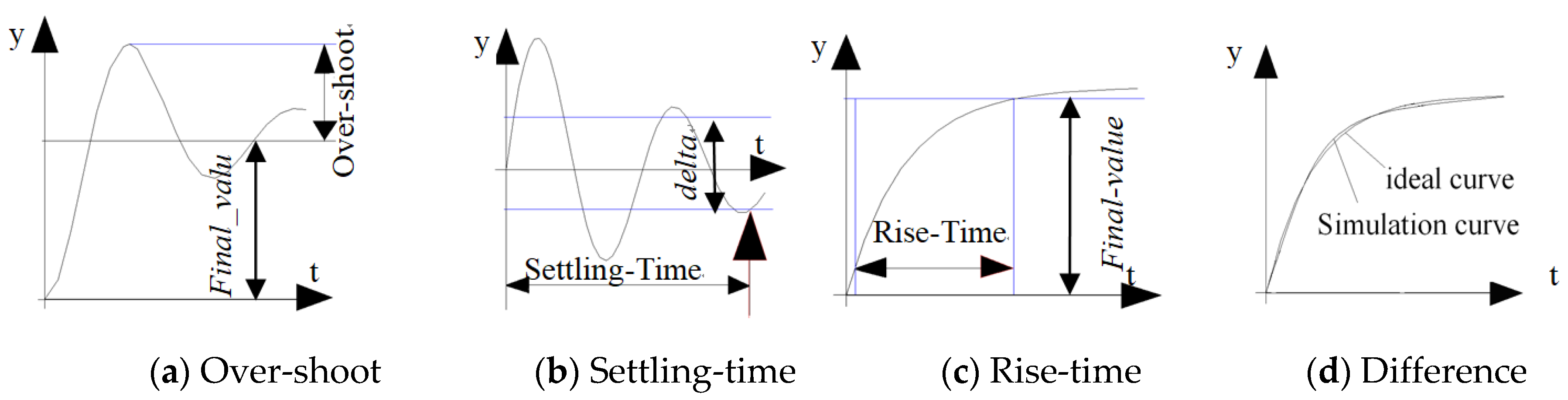
28]: over-shoot, settling-time, and rise-time. As shown in
Figure 3a, the parameter final_Value is the desired reference value of the input signal y. The over-shoot is defined as max (0, y—Final_value), i.e., the largest value of y over the Final_value. Settling-time (
Figure 3b) is the first time where the input signal y remains within a range of delta forever. Also, rise-time (
Figure 3c) computes the rise time of the input signal. Generally, it is the time between the input signal being equal to 0.1 * Final_value and 0.9 * Final_value.
In addition, the difference (
Figure 3d) between the ideal curve and the simulation response curve of a variable should be considered under the condition of parameter estimation. The ideal curve can be given with pairs of value-time series. The difference value can be calculated through interpolation. To make the difference of two curves minimize is to minimize the sum of all the squares of differences between ideal values and response values at the discrete time sequences.
3.2. Optimization Modeling for a Modelica Model with Multi-Cases
By using a suitable search algorithm to minimize some objective functions and satisfy some constraints, the Optimization based on Modelica is can find a set of optimal parameters of a Modelica model. The Modelica model is called a “main simulation model”, which should be a Modelica class or model in which the number of variables is equal to the number of equations.
As we know, an optimization model has three aspects: design variables (or tuners), constraints, and objective functions. As for the simulation optimization for a Modelica model, generally tuners are the parameters of the main simulation model or parameters of its components of sub-components. A tuner has three main data members: default value, minimum, and maximum value. The default values of tuners are the initial values when optimizing; maximum and minimum values of tuners are boundary constraints of the optimization model.
In order to avoid evaluating values of expressions of user-defined design functions (constraints and objective functions), we can define them as some output variables in the model text. Then, values of design functions can be evaluated through these output variables, which can be resolved when simulating. Because the design functions often include state variables, the corresponding output variables should be set with different criteria, as mentioned in
Section 3.1.
If we optimize a model that has a different typical work status or structures, the multi-case optimization model can be used [
28]. Cases describe different operating conditions that are distinguished by different values of a set of parameters, namely, case parameters. Generally, case parameters are discrete parameters and are kept at a fixed value in a case. One case has one set of case parameters. Multi-case optimization modeling means that when optimizing a model, all the objective functions and constraints of all the cases must be considered. Thus, the multi-objects optimization and multi-constraints optimization are two core parts in multi-case optimization.
Multi-objects of multi-cases can be aggregated into one object according to the weight of each object of each case. The sum of the absolute of each weighted object is a common aggregation method. Then, the multi-case optimization model can be described as follows:
where
X denotes tuners;
F,
I, and
E denote the set of objective functions, inequality constraints, and equality constraints in cases, respectively, i.e.,
fij denotes the
ith object in the
jth case. In order to achieve the same scale of different objective functions, a fixed demand value (
dij,
) is needed for each object in each case. A demand value has the same unit as its corresponding object, which denotes the designer’s preferences. Moreover,
is the overall object function of multi-objects of multi-cases.
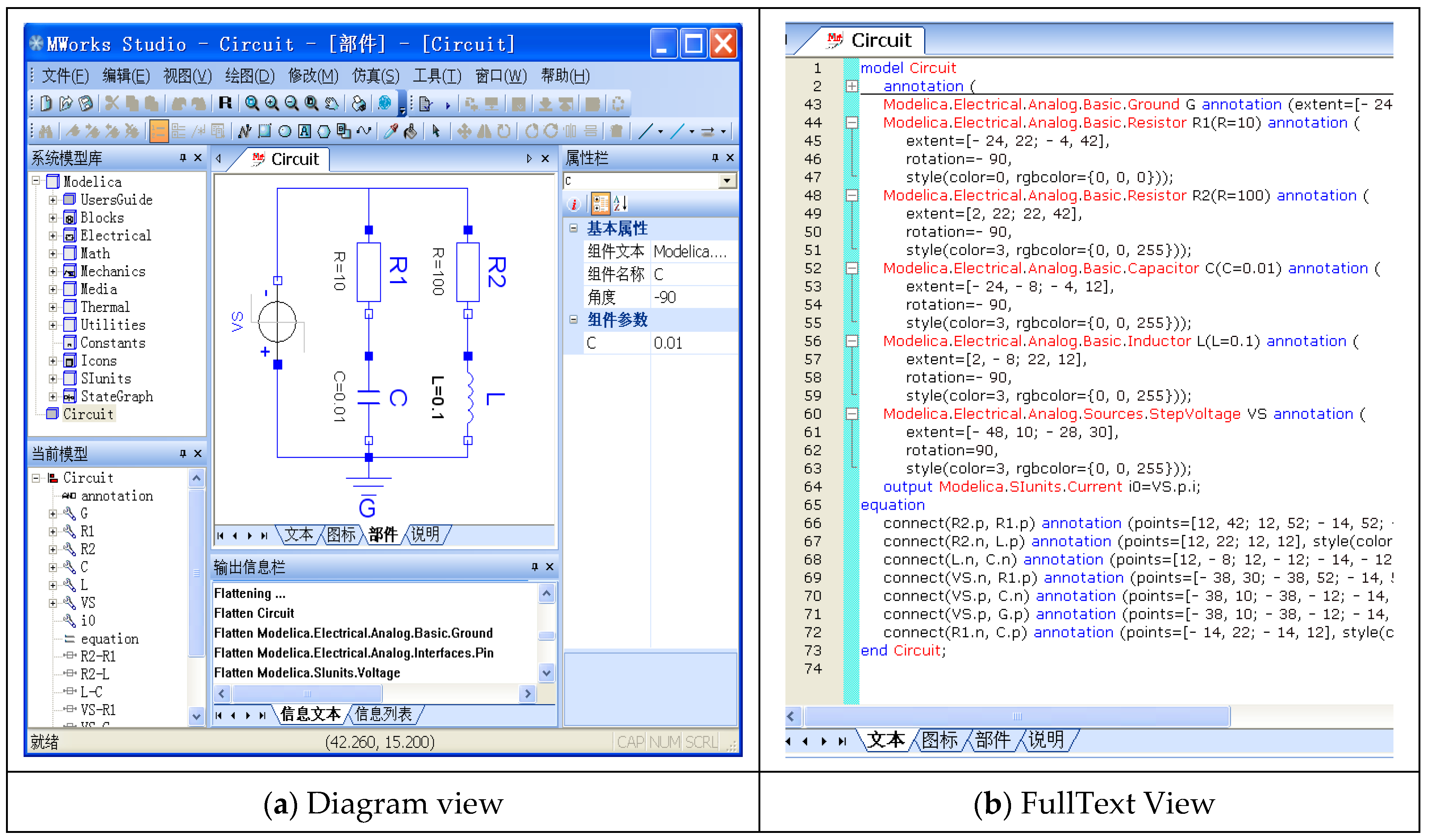
As for the circuit model of
Figure 1, we consider the following optimization problem:
find: {C.C, L.L}min: Difference (i0, Ij ), j = 1,2,3; dj = 1;s.t. settling-time (i0) < Tj, j = 1,2,3over-shoot(i0) ≤ Aj, j = 1,2,3cases: {R1.R, R2.R} = {20, 100; 50, 50; 100, 20}{T1, T2, T3} = {2, 3, 4}{A1, A2, A3} = {0, 0, 0}
where
C.C is the value of the capacitor
C;
L.L is the value of the inductance
L; and
i0 is the overall current of the circuit. There are three cases in the model with different case parameters
R1.R and
R2.R.
I1,
I2,
I3 are three ideal current curves corresponding to the three cases, respectively, and they are given with a series of value-time pairs.
3.3. Parameter Optimization Process
As mentioned in the previous sections, a physical system described by
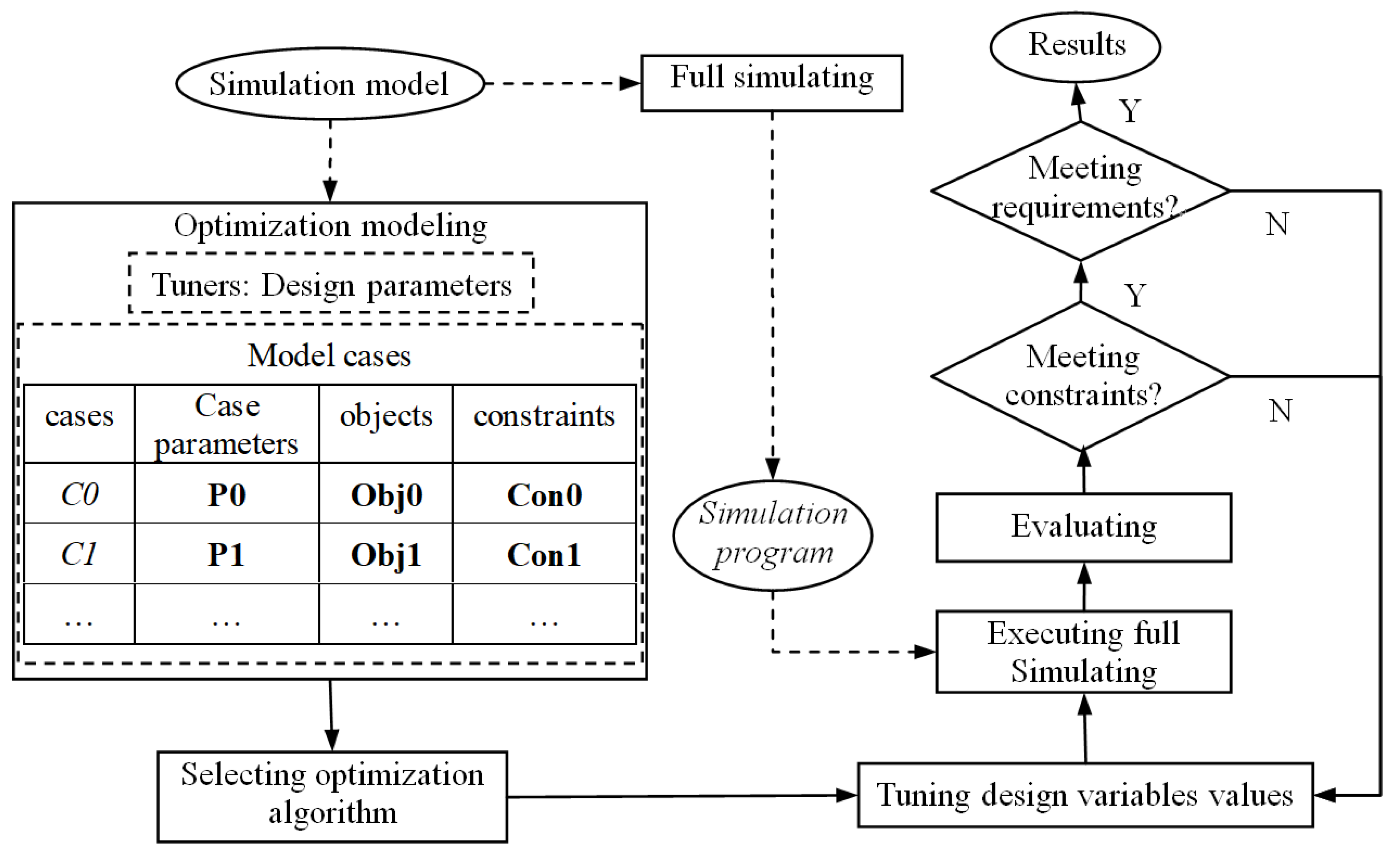
Modelica can be defined as a parameterized simulation model. Therefore, design optimization can be employed to tune parameters such that the system behavior is improved. After setting up an optimization model for a
Modelica simulation model, a search algorithm (such as SQP-sequential quadratic programming, Hookjeeves, GA-genetic algorithm, etc.) is used to constantly adjust design variables, execute the simulation program and evaluate the design functions in order to minimize the objective functions and meet the constraints. The process of design optimization based on
Modelica model is illustrated in
Figure 4.
As shown in
Figure 4, the optimization model including design variables, case parameters, objective functions, and constraints is built from the
Modelica simulation model. Before iteration of optimization, a full simulation program is generated. During each iteration, the simulation program is then called after tuning the values of design variables. If the model has multi cases, a simulation program would be called several times (equaling to the number of cases) with different sets of values to the case parameters during one iteration step. Assume the number of cases is
nCases, and the number of the optimization iterations is
nIters, then the simulation will run
nCases * nIters times during the whole optimizing process. After simulation, criteria of the state variables in the objective functions or constraints will be evaluated according to the simulation results. A more specific process may be referred to in [
9].
4. Partial Resolving Algorithm for a Modelica Model
As we know, many repetitive simulations must be executed during optimizing, especially for a multi-case optimization model. Thus, if the simulation program could be shortened, a great deal of time could be saved. Under MWorks, we adopt a method named “minimum simulation” in which full resolving is substituted with partial resolving.
The random geometric graphs [
29] have been well-studied and applied to alternative mechanisms wrapped in real-world complex networks. In addition, the idea on the sorted blocks is interesting. It can potentially be used to structure insightful hierarchical structures. Shang [
30] studied a model for inhomogeneous long-range percolation on the hierarchical lattice
of order
with an ultrametric
. The random geometric graphs and the idea on the sorted blocks are helpful for researchers to further understand the partial resolving algorithm.
Note that this method can only be used under the condition that the equation system of the simulation model does not change when tuning the parameters. If the structure of the equation system changes, all the variables, the solving dependency graph, and the MSG could also change.
4.1. Solving Dependency Graph
Definition 1. Coupling block, a set of tightly coupling simultaneous equations that can be solved independently. A coupling block has five domains:s_sEqu represents the set of equations; s_sPar represents the set of parameters; s_sVar represents the set of output variables which will be resolved through this block; s_pParents represents the set of pointers of parent blocks which should be resolved before; and s_pChildren represents the set of pointers of children blocks which depends on this block. Pre-blocksof a block B is the blocks that are B’s parents or their parents, recursively.
Post-blocksof a block B is the blocks that are B’s children of their children, recursively.
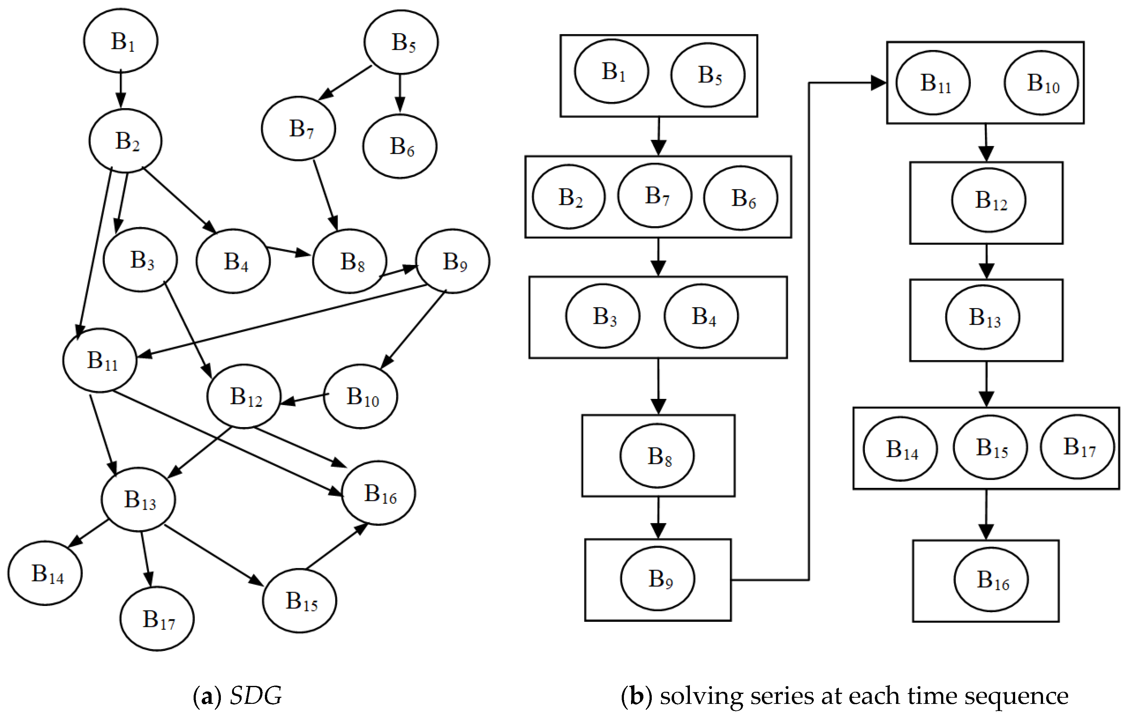
Definition 2. Solving a dependency graph is a graph which is defined as follows:Vertices B in the solving dependency graph (SDG) is a set of coupling blocks and the edgeindicates the data dependence between vertices B1 and B2. That is, there exists at least one variable v in B2 whose value is computed in B1. This type of variable (such as v) is called as computation variables in B1 and is also known as reference variables in B2, i.e., B1 is B2′s parent. Considering the circuit model in
Figure 1, we can easily build
SDG of the 17 sorted blocks of the equation system when performing topological sorting of the equation system into BLT form—all the nodes in one strongly connected component construct a block. As
Figure 5a shows, a solving dependency graph is a directed graph without loops.
Once the
SDG of an equation system is built, we can easily obtain the computing sequences through erasing the parent blocks [
9], as shown in
Figure 5b. Blocks in the same rectangle can be resolved in a random order.
4.2. Minimum Solving Graph
Once the optimization model is built, we can construct its minimum solving graph based on the SDG. This method is based on the idea that if all the variables are resolved at first, we just need to resolve the blocks which are related to the optimization model. During the optimization iteration process, the simulation objective is to evaluate the values of objective functions and constraints according to the tuners and case parameters. Thus, the minimum solving graph is the sub-graph of SDG from the blocks of the tuners and case parameters to the blocks of constraints and objective functions.
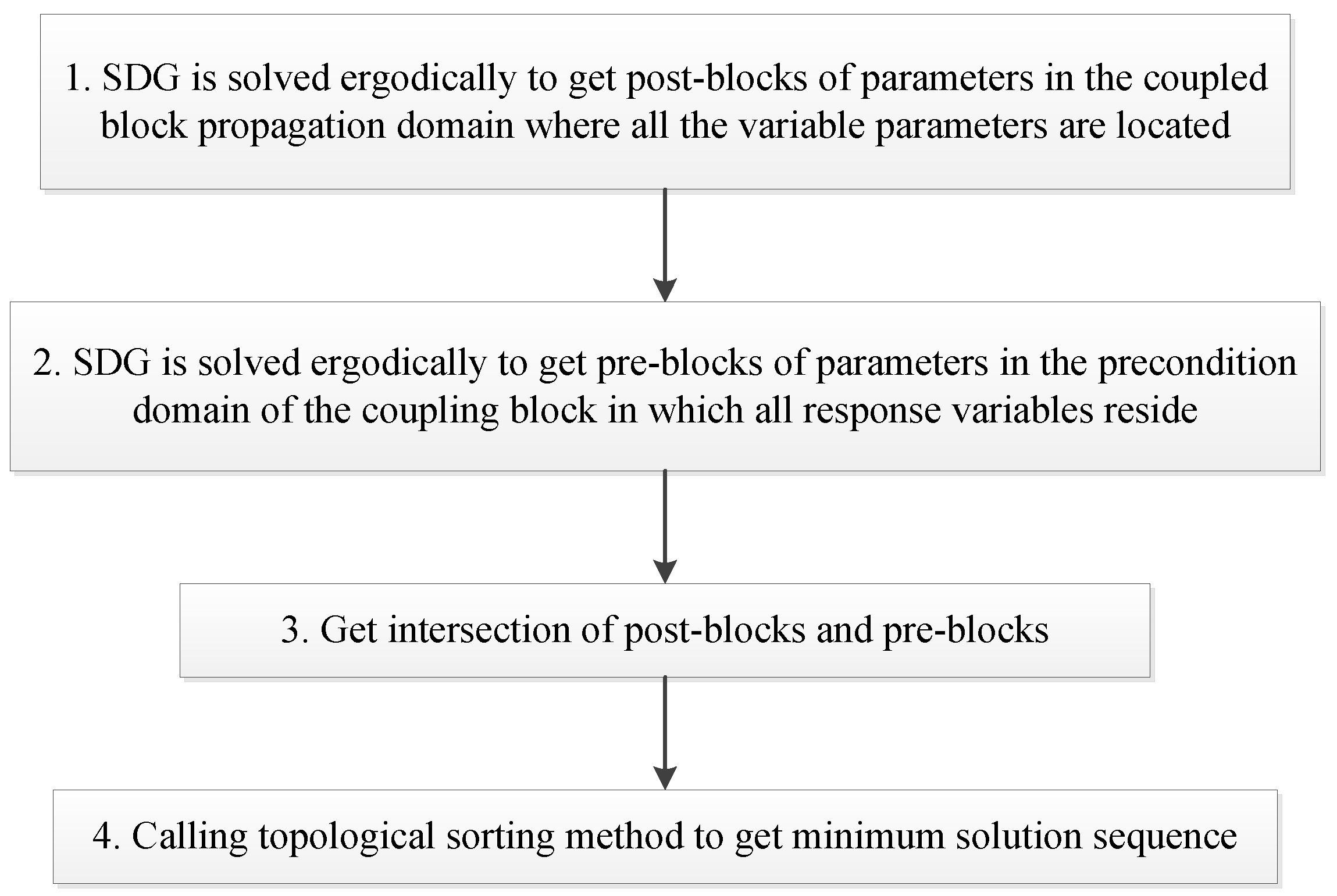
The following are the three steps required to construct the minimum solving graph: getting the sub-graph coving post-blocks of parameters (including tuners and case parameters) in which all the blocks are affected by these parameters; getting the sub-graph coving pre-blocks of constraints or objective functions in which all these blocks affect blocks of objective functions or constraints; getting the intersection of the two sub-graphs. This intersection sub-graph is the very minimum solving graph. Given
GP is the post-blocks of parameter
par1,
par2,
par3,
…;
GO is the pre-blocks of objects
obj1,
obj2,
obj3; and
GC is the pre-blocks of constraints
con1,
con2,
con3, …; then the minimum solving process is shown in
Figure 6.
The specific algorithm implemented can be stated as follows:
The following Algorithm 1 illustrates the procedure of getting post-blocks of parameters:
| Algorithm 1. GetParPostBlocks |
| Input: s_strPar – a set of parameters |
| SDG – solving dependency graph |
| Output: s_pBlks – set of post-blocks selected |
| for each block b in SDG do begin |
| if intersection of b.s_Par and s_strPar is null or b is in s_pBlks then continue; |
| clear set s; |
| s = GetSuccesor (b, SDG, s_pBlks); //get successors of b in SDG |
| Add s to s_pBlks; //select s |
| end for; |
In order to improve the efficiency of the algorithm, the GetSuccessor function (Algorithm 2) is passed with the set of blocks s_pBlks which have been selected:
| Algorithm 2. GetSuccesor |
| Input: b – the block |
| SDG – solving dependency graph |
| s_pBlks – set of blocks which has been selected |
| Output: s_pSucBlks – set of blocks selected |
| clear set s; |
| s = b.s_children; |
| for each block b1 in s do begin |
| if b1 is in s_pBlks then continue; |
| clear set s1; |
| GetSuccesor ( b, SDG, s_pBlks); //call itself recursively |
| Add b1 to s_ pSucBlks; |
| end for; |
Similarly, the following Algorithm 3 illustrates the procedure of getting pre-blocks of variables:
| Algorithm 3. GetVarPreBlocks |
| Input: s_strVar – a set of Variables |
| SDG – solving dependency graph |
| Output: s_pBlks – set of blocks selected |
| for each block b in SDG do begin |
| if intersection of b.s_Var and s_strVar is null or b is in s_pBlks then continue; |
| clear set s; |
| s = GetProccesor(b, SDG, s_pBlks); //Get Processors of b in SDG |
| Add s to s_pBlks; //select s |
| end for; |
Like the function GetSuccessor, Getsuccessor function (Algorithm 4) is also passed with the set of blocks s_pBlks:
| Algorithm 4. GetProccesor |
| Input: b – the block |
| SDG – solving dependency graph |
| s_pBlks – set of blocks which has been determined |
| Output: s_pProBlks – set of blocks |
| clear set s; |
| s = b.s_parents; |
| for each block b1 in s do begin |
| if b1 is in s_pBlks then continue; |
| clear set s1; |
| GetProccesor ( b, SDG, s_pBlks); //call itself recursively |
| Add b1 to s_ pProBlks; |
| end for; |
The following Algorithm 5 illustrates the procedure of getting an intersection of two sets of blocks:
| Algorithm 5. GetMSGBlocks //getting set of blocks in a MSG |
| Input: s_pParBlks—set of post- blocks of parameters |
| s_pVarBlks—set of pre-blocks of output variables appearing in the objective functions or constraints functions |
| Output: s_pMSGBlks—set of blocks in a MSG |
| for each block b in s_pParBlks do begin |
| if b is in s_pParBlks then |
| add b to s_pMSGBlks; |
| end for |
Algorithm 5 only gets the set of blocks in a MSG, the next algorithm, Algorithm 6, gets the series of sorted blocks:
| Algorithm 6. GetSortedBlocks |
| Input: s_pMSGBlks – set of blocks in a MSG |
| Output: v_ pMSGBlks – vector of sets of blocks which are sorted |
| while s_pMSGBlks in not null do begin |
| for each block b in s_pMSGBlks do begin |
| clear set s; |
| if intersection of b.s_pParents and s_pMSGBlks is null then |
| add b to s; |
| end for; |
Up until now, all the algorithms to build a partial simulation program based on an MSG have been narrated. The main procedure of generating a series of blocks of an MSG is illustrated as the following algorithm, Algorithm 7:
| Algorithm 7: GenerateMSGSortedBlocks |
| //generating minimum solving series of blocks in MSG |
| InputSDG, s_pars, s_Vars |
| Outputv_setMSGBlks |
| Step1: s_pBlk1 = GetParPostBlocks (SDG, s_pars); |
| Step2: s_pBlk2 = GetVarPreBlocks (SDG, s_Vars); |
| Step3: s_pMSGBlks = GetMSGBlocks (s_pBlk1, s_pBlk2); |
| Step4: v_pMSGBlks = GetSortedBlocks (s_pMSGBlks); |
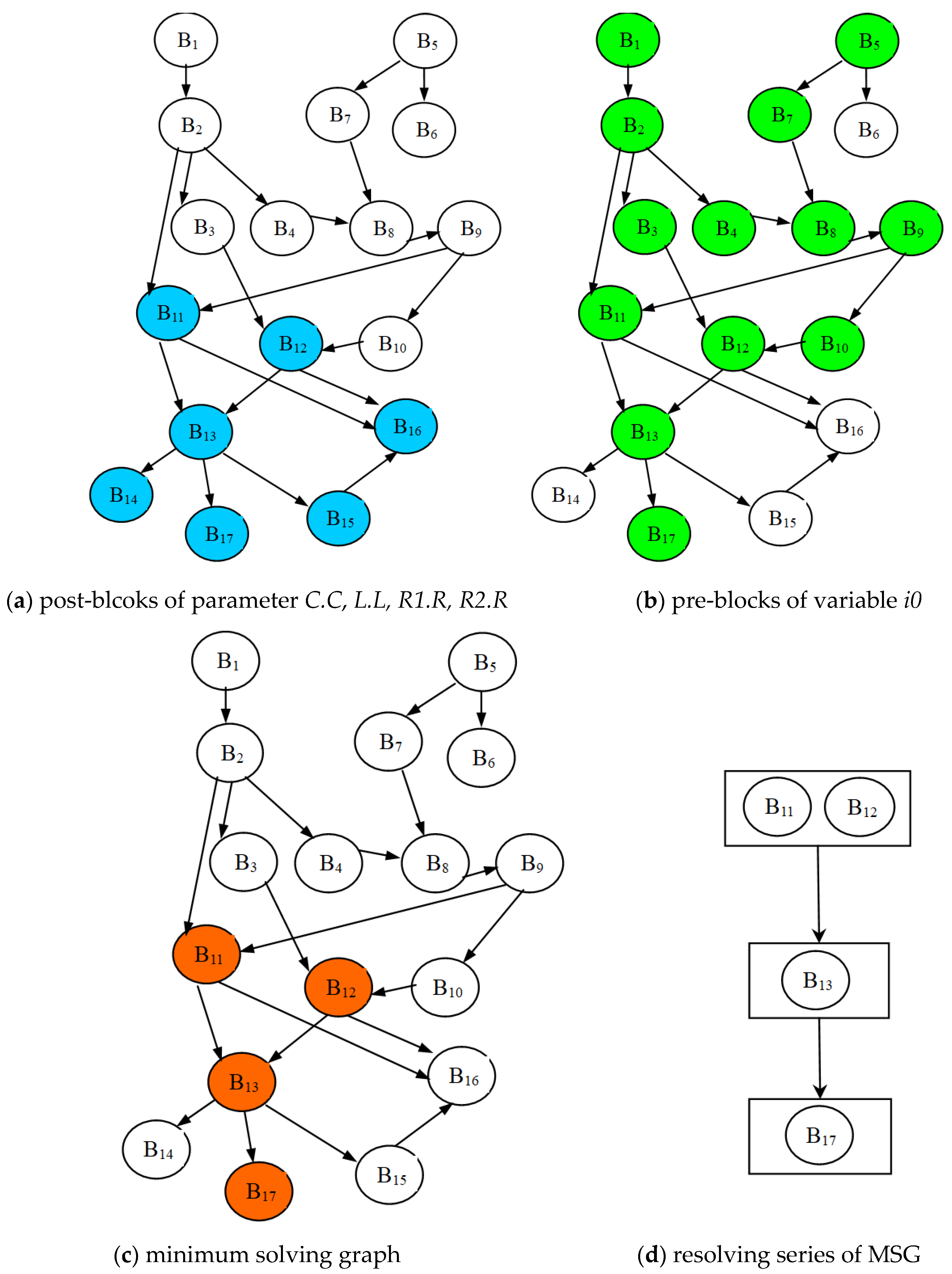
Using the algorithm above, we can build the minimum solving graph of the circuit model of example 1 as
Figure 7 shows.
Figure 7a–d illustrates Algorithms 1–4, respectively. The results of the sorted blocks are {B
11 | B
12, B
13, B
17}.
4.3. Optimization Iteration Process Based on Minimum Simulation
The minimum simulation program now can be built from the series of blocks of the MSG. When generating a minimum simulation code, the full simulation results resident in memory must be used to resolve the variables whose values changed in the MSG. All the values of unvaried variables are obtained at first through dynamics data exchange. In order to ensure all the values of all these variables at discrete time sequences have been saved, simulation steps must be matched between the partial resolving and full simulation. Thus, we adopt a constant steps (or the same varied steps) strategy in both the full simulation and minimum simulation code by setting the output interval to “interval length”.
Based on the minimum simulation program, the process of parameter optimization has been improved, as
Figure 8 shows. From the simulation model and the optimization model, the MSG is built at first. Then, full simulation is called only once to generate the full results in a mat file. According to the MSG and the full results, the minimum simulation program is finally built. Then, a simulation before evaluating the values of constraints and objective functions only needs to execute the minimum simulation program.
As mentioned above, the MSG is built not only by design parameters but also case parameters. As for the multi-case optimization model, another method of partial resolving is to build several different full simulation programs (the number of which equals the number of cases) according to different sets of values of the case parameters firstly, then constructing the minimum solving graph based only on the tuners (excluding case parameters), and lastly building several minimum simulation programs (number of which also equals to the number of cases). Thus, when evaluating the values of design functions of multi-cases, the multi minimum simulation programs will be called, respectively. The more efficient this method is, the greater the number of pre-blocks of case parameters and of optimization iterations is.
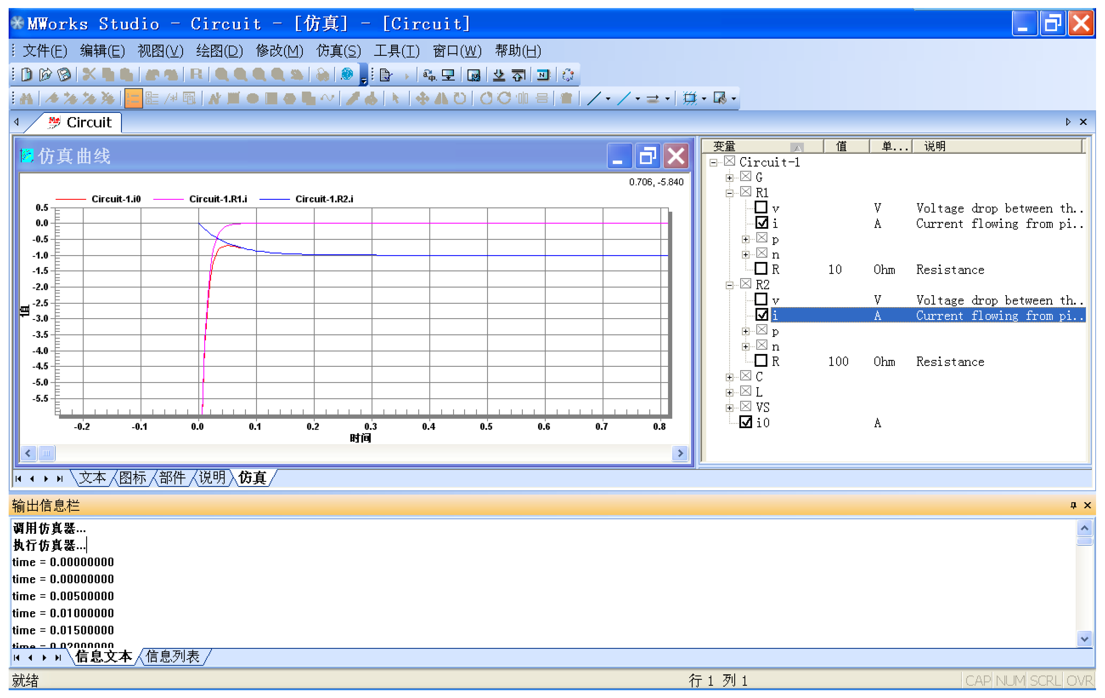
As for the optimization problem of the circuit example, we can get the optimal result, {
C.C,
L.L} = {0.033F, 0.0004H}, with the curves of the
i0 ideal current and simulation response being shown in
Figure 9. Using partial resolving during the optimization process can save time at about 10% when contrasted with full simulation. Actually, the different optimization models have different MSG. If we only select C.C as the tuners, then the MSG has only three blocks: B
11, B
13, and B
17. Accordingly, the consuming time of the optimization could be reduced by 45%. However, if we select the parameter VS.signalSource.p_height as tuners, its MSG then covers nearly all the blocks, except four blocks: B
1, B
2, B
3, and B
4. This means time of partial resolving is close to that of the full simulation.
5. Application
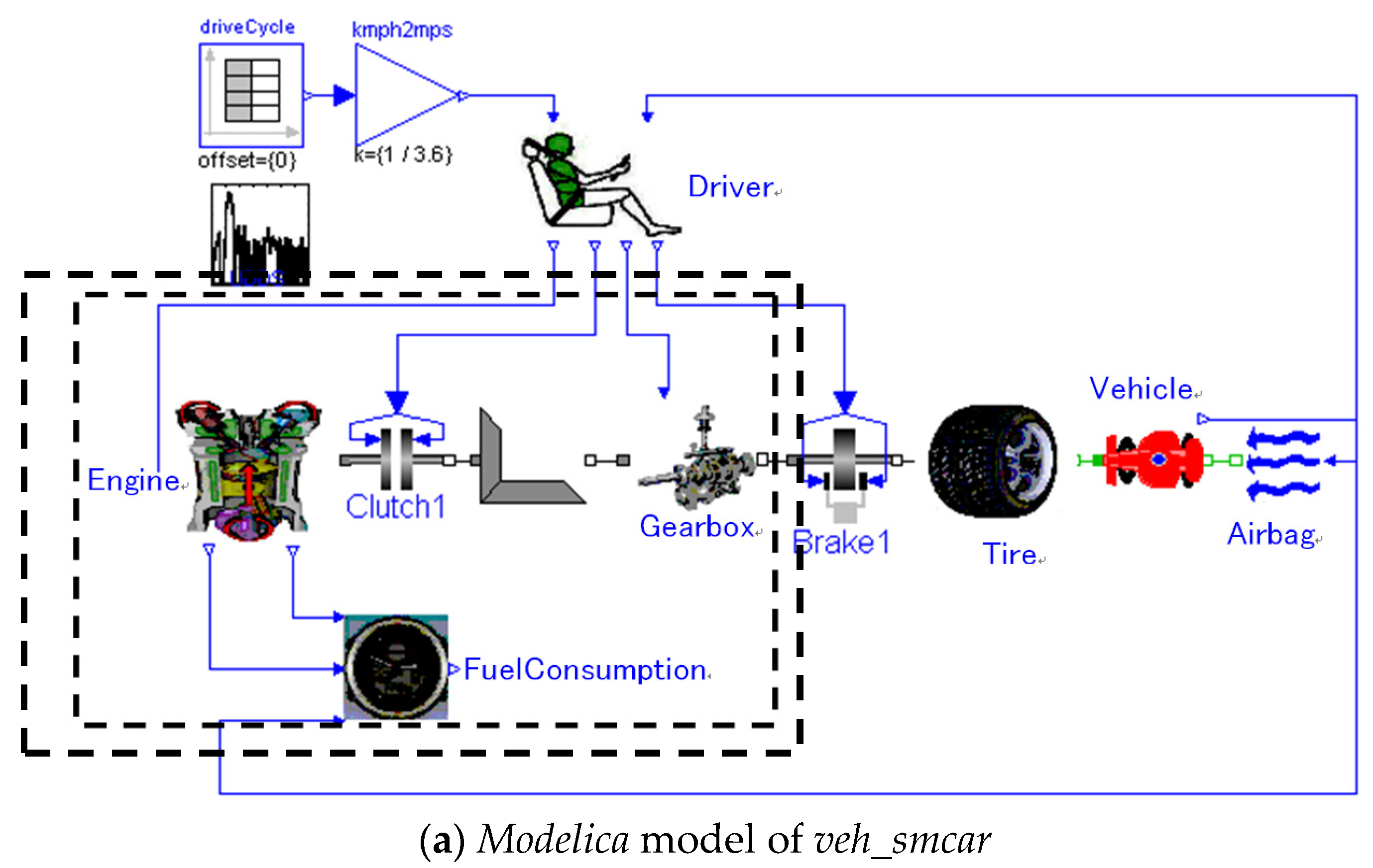
In order to save energy effectively, the economy of fuel is now given more and more consideration when designing vehicles, especially heavy trucks. Collaborating with Chinese Heavy Truck Corp., our group has built a
Modelica library—InteDrive—to facilitate modeling and simulating for a heavy truck model. InteDrive includes the following sub-libraries: driveCycle, Driver (including BrakeControl, ThrottleControl, ShiftStrategy), engine, clutch, gearbox, brake, tire, vehicle, airbag, and fuel consumption. Based on the InterDrive library, a sample model of heavy truck—
veh_smcar—has been built under MWorks, as
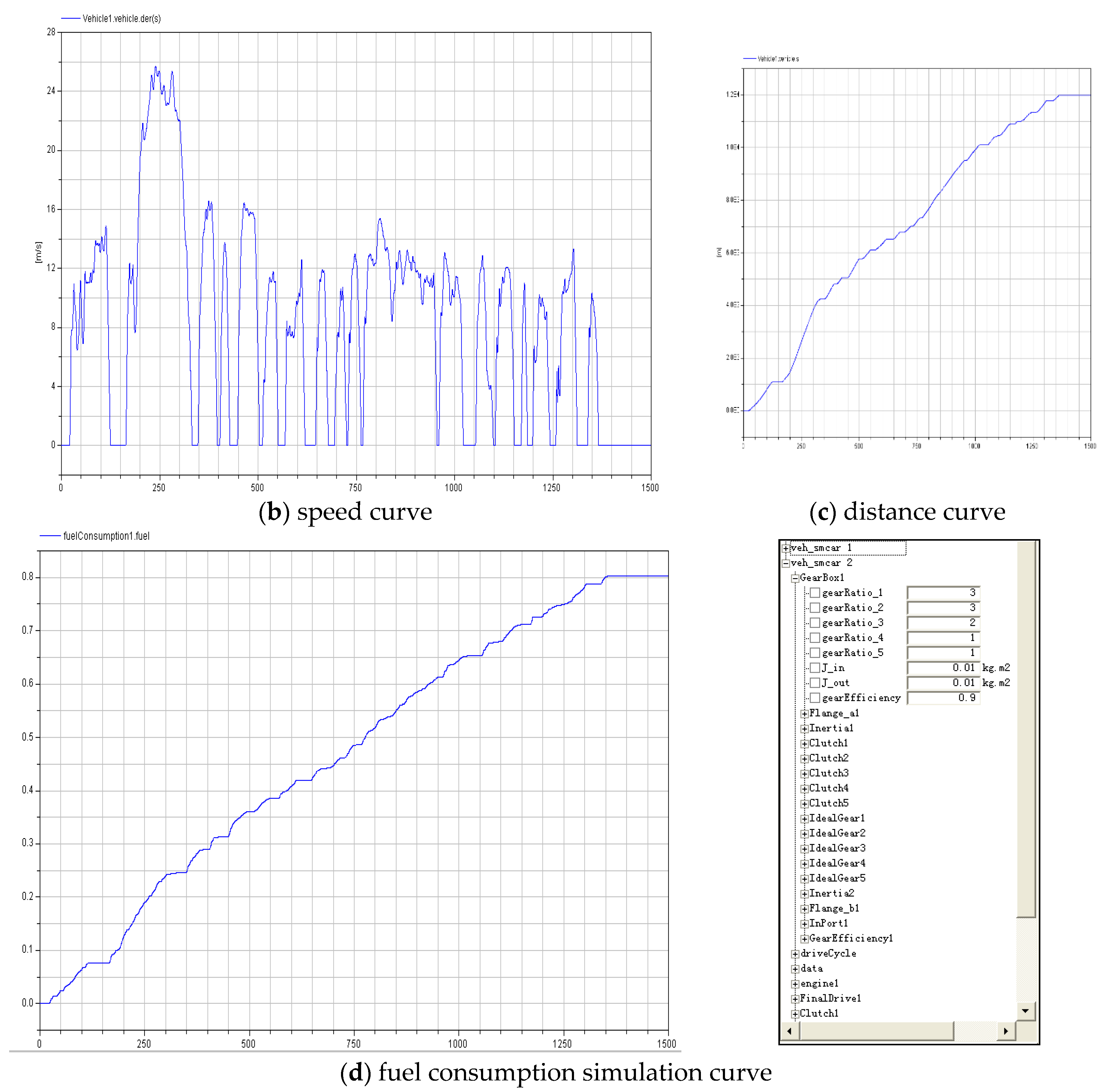
Figure 10a shows.
Under the MWorks platform, some main simulation curves can be obtained by setting the parameters:
GearBox1.gearRatio_1 = 3,
GearBox1.gearRatio_2 = 3,
GearBox1.gearRatio_3 = 2,
GearBox1.gearRatio_4 = 1, and
GearBox1.gearRatio_5 = 1, and adopting the predefined shift strategy of the component
Driver:
parameter Real upshift[:] = {25, 50, 70, 100} "upshift table,(km/h)";parameter Real downshift[:] = {20, 40, 60, 90} "downshift table,(km/h)";Modelica.Blocks.Interfaces.InPort vehicle_speed;Modelica.Blocks.Interfaces.OutPort requested_gear_number;Integer current_gear(start = 1);Integer speeds = size(upshift,1) + 1;Real next_upshift;Real next_downshift;initial algorithmcurrent_gear = 1;next_upshift = if current_gear < speeds then upshift[current_gear] else Modelica.Constants.inf;next_downshift = if current_gear > 1 then downshift[current_gear - 1] else -Modelica.Constants.inf;algorithmwhen vehicle_speed.signal[1] > next_upshift thencurrent_gear : = current_gear+1;next_upshift : = if current_gear<speeds then upshift[current_gear] else Modelica.Constants.inf;next_downshift : = if current_gear>1 then downshift[current_gear-1] else -Modelica.Constants.inf;end when;when vehicle_speed.signal [1] < next_downshift thencurrent_gear : = current_gear-1;next_upshift : = if current_gear<speeds then upshift[current_gear] else Modelica.Constants.inf;next_downshift : = if current_gear>1 then downshift[current_gear-1] else -Modelica.Constants.inf;end when;After simulation, the curves of vehicle speed, distance, and fuel consumption in 1500s are shown in
Figure 10b–d, respectively. Total fuel consumption of
veh_smcar in 1500 s was 8.1 L.
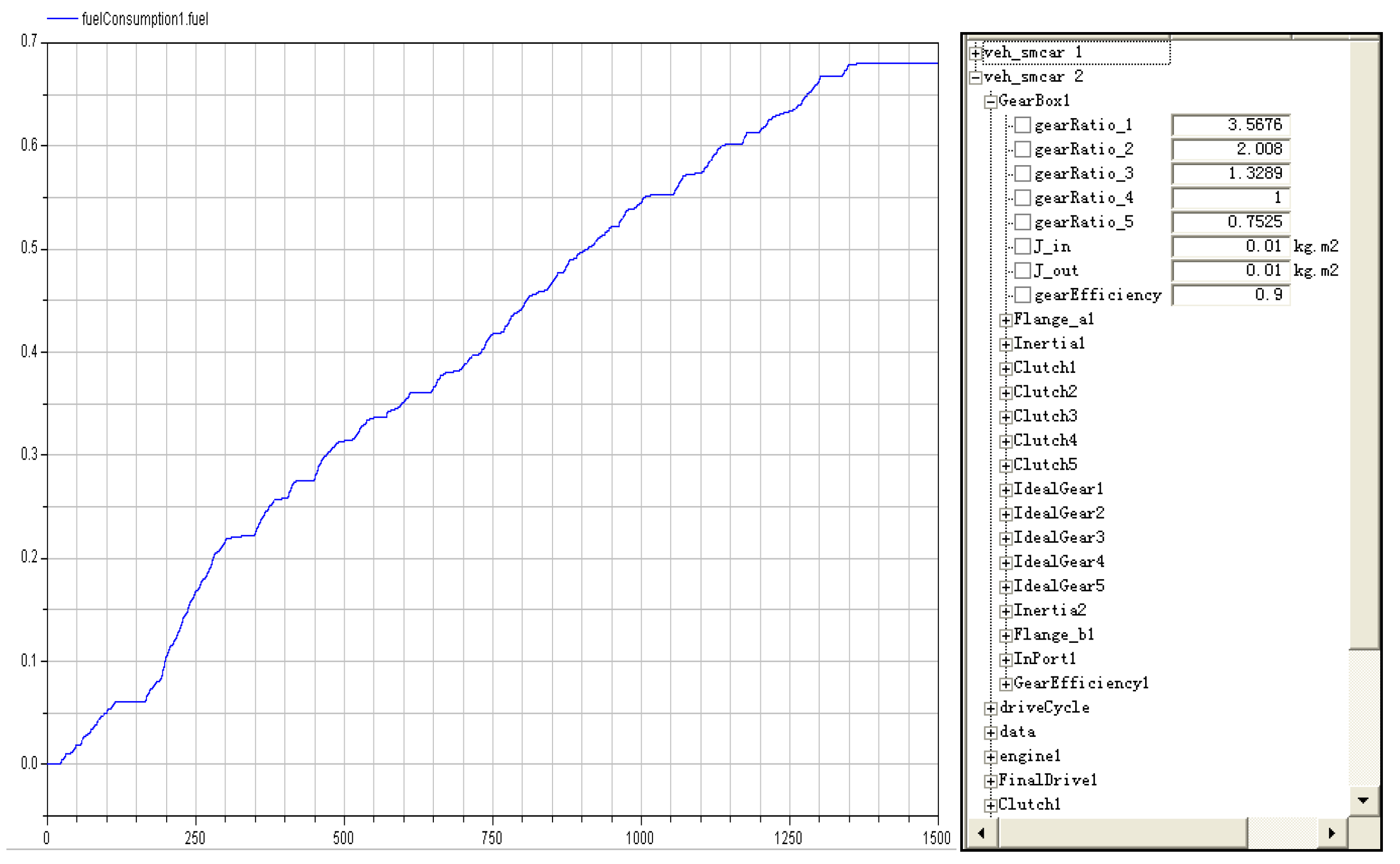
Next, we set up the optimization model:
find {gearRatio_1, gearRatio_2, gearRatio_3, gearRatio_4, gearRatio_5}min: fuelComsumption1.fuels.t. max (vehicle1.speed) < Vj, j = 1,2,3cases: three common shift strategies with different sets of table values of upshift and downshift.{upshift1, upshift2, upshift3} = {{25, 50, 70, 100}, {30, 55, 80, 110}, {20, 45, 65, 95}}{downshift1, downshift2, downshift3} = {{20, 40, 60, 90}, {25, 50, 70, 100}, {15, 40, 60, 90}}{V1, V2, V3} = {90 km/h, 100 km/h, 110 km/h}After optimizing, the optimal values of tuners are as follows:
GearBox1.gearRatio_1 = 3.57,
GearBox1.gearRatio_2 = 2.01,
GearBox1.gearRatio_3 = 1.33,
GearBox1.gearRatio_4 = 1.00, and
GearBox1.gearRatio_5 = 0.75. The total fuel consumption was about 6.8 L. The fuel simulation curve in 1500 s is shown in
Figure 11.
By using the SQP algorithm, there are 12 iterations during the optimizing process. If simulation time is set up from 0 to 1500 s, the consuming time for full simulation is about 9.8 s under MWorks. After generating a minimum solving graph according to the optimization model, each partial simulation time is about 5.6 s. Therefore, more than one third of time taken can be saved during the optimization process. As
Figure 9a shows, only the variables in the dashed rectangle should be resolved when executing the partial simulation.
As for the veh_smcar model, if we select parameters in the component Engine (like fc_inertia) as tuners, its MSG will decrease greatly, while if we select parameters in the component driveCycle, such as the matrix table, then its MSG covers all the solving blocks.
6. Conclusions
Parameter optimization for a Modelica model needs to execute simulation repeatedly in order to evaluate design functions, and the efficiency of the process of design optimization depends on the efficiency of repetitious simulation to a great extent. Although there are many studies focusing on solving strategies of simulation, few of them pay attention to the efficiency of repetitious simulation after parameter tuning. Because only the equation blocks from design parameters to design functions of an optimization model need to be resolved during iterations, a minimum solving graph and partial resolving strategy based on a simulation model and optimization model is presented in this paper. By using this method, the more efficient it could be, the smaller the size of the MSG. Also, it would be useful for a model experiment with parameter tuning or parameter estimation.
For next study of this work, we are trying to generate several full simulation codes, corresponding MSGs and minimum simulation programs before optimizing. When executing partial simulation, the main optimization program calls one suitable minimum simulation program according to the values of parameters. Furthermore, a multiscale filtering algorithm and concept of network robustness [
31] in the multiscale coordination control problem will be introduced to effectively guide us to enhance the efficiency and performance of the partial simulation resolving algorithm to a certain extent.


