Multivariable System Identification Method Based on Continuous Action Reinforcement Learning Automata

Abstract
:1. Introduction
2. Materials and Methods
2.1. Background
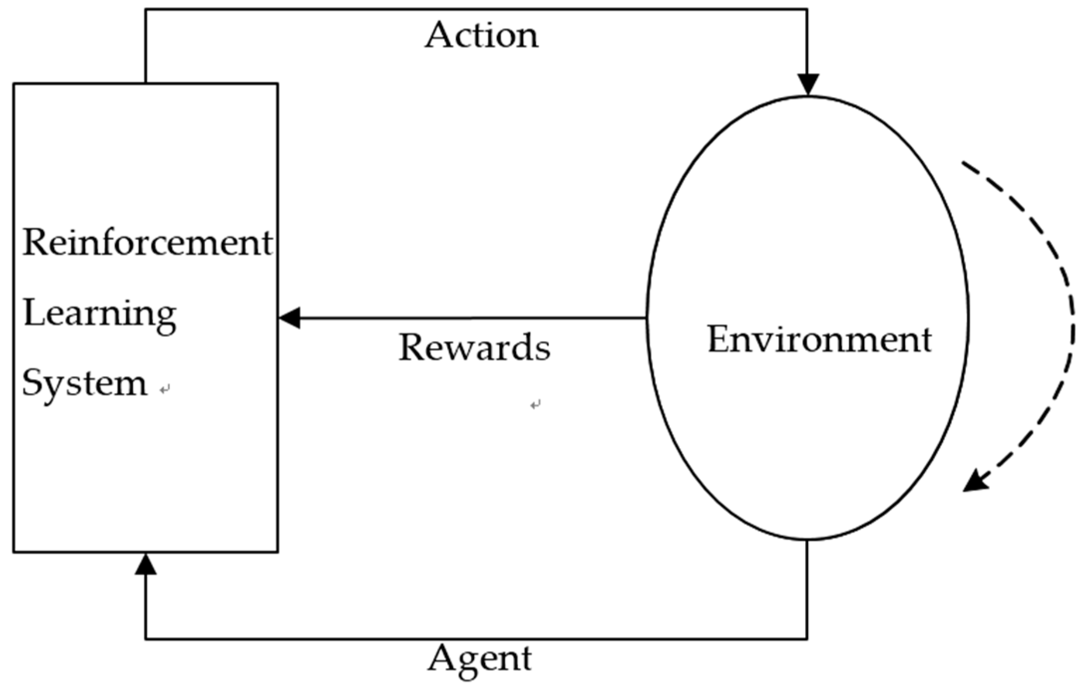
2.2. Basic Reinforcement Learning
2.3. Continuous Action Reinforcement Learning Automata (CARLA)
| CARLA algorithm |
| 1: Initialize the probability density function : establish the uniform distribution of CPDFs according to the range of the parameter; |
| 2: Actions selection: select actions (or parameters) randomly based on the CPDF value; |
| 3: System evaluation: take the action, substitute parameters into the system to obtain the responding curve, and calculate the fitness function ; |
| 4: Calculate the enhanced signal value according to the value of the fitness function; |
| 5: Update each CPDF value according to the enhanced signal value; |
| 6: Update behavior parameters: introduce the normal random number generator to update the action parameters at the next moment; |
| 7: If the stopping condition has not been reached, return to step 2 until the convergence condition is met. |
3. Frequency Response Estimation Based on CARLA (CARLA-FRE)
3.1. Frequency Response Estimation Based on CARLA (CARLA-FRE)
3.2. The Applications of CARLA-FRE in MIMO Systems
3.2.1. Closed-Loop Identification for Square Multivariate Systems
3.2.2. Closed-Loop Identification for Non-Square Multivariate Systems
4. CARLA Algorithm Performance Verification
5. Simulation
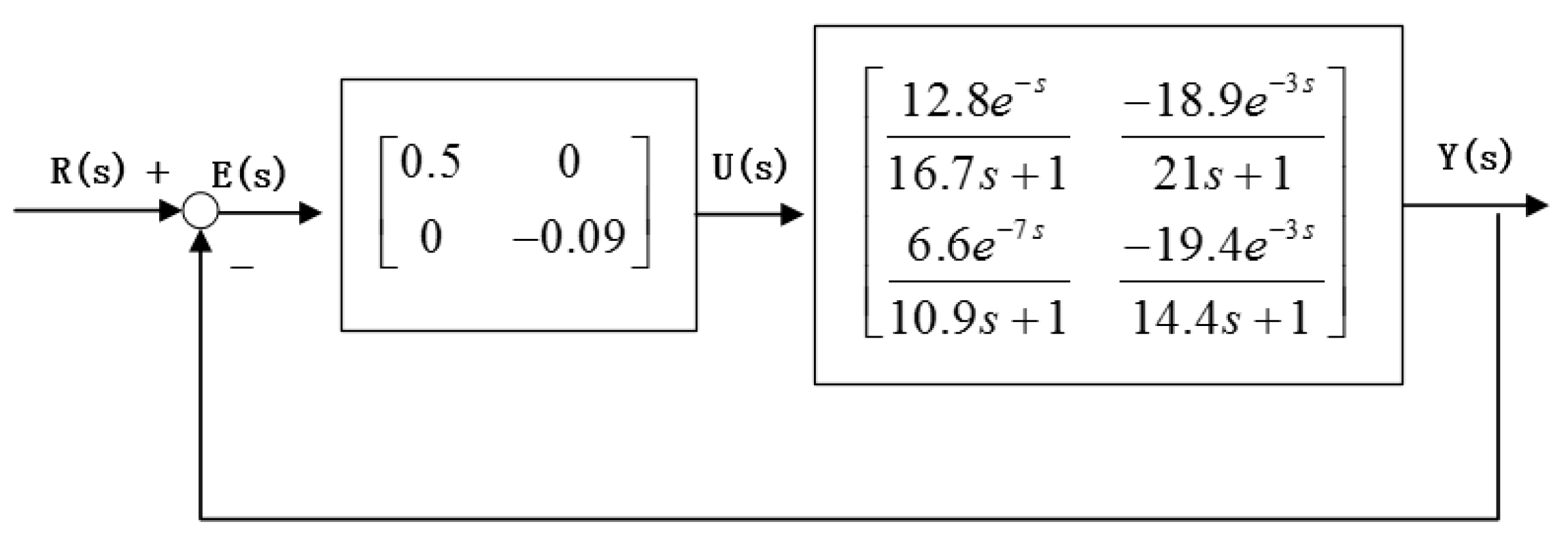
5.1. Square Multivariate System: Wood-Berry Model
5.2. Non-Square Multivariate System: Shell Model
6. Conclusions
Author Contributions
Funding
Acknowledgments
Conflicts of Interest
References
- Gupta, R.D.; Fairman, F.W. Parameter estimation for multivariable systems. IEEE Trans. Autom. Control 1974, 19, 546–549. [Google Scholar] [CrossRef]
- Guidorzi, R. Canonical structures in the identification of multivariable systems. Automatica 1975, 11, 361–374. [Google Scholar] [CrossRef]
- Verhaegen, M. A novel non-iterative mimo state space model identification technique. IFAC Proc. Vol. 1991, 24, 749–754. [Google Scholar] [CrossRef]
- Nakayama, M.; Oku, H.; Ushida, S. Closed-loop identification for a continuous-time model of a multivariable dual-rate system with input fast sampling. IFAC PapersOnLine 2018, 51, 415–420. [Google Scholar] [CrossRef]
- Moor, B.D.; Overschee, P.V. Numerical algorithms for subspace state space system identification. In Trends in Control; Springer: London, UK, 1995. [Google Scholar]
- Gumussoy, S.; Ozdemir, A.A.; McKelvey, T.; Ljung, L.; Gibanica, M.; Singh, R. Improving linear state-space models with additional niterations. IFAC PapersOnLine 2018, 51, 341–346. [Google Scholar] [CrossRef]
- Larimore, W.E. Canonical variate analysis in identification, filtering, and adaptive control. In Proceedings of the 29th IEEE Conference on Decision and Control, Honolulu, HI, USA, 5–7 December 1990; pp. 596–604. [Google Scholar]
- Pilario, K.E.S.; Cao, Y.; Shafiee, M. Mixed kernel canonical variate dissimilarity analysis for incipient fault monitoring in nonlinear dynamic processes. Comput. Chem. Eng. 2019, 123, 143–154. [Google Scholar] [CrossRef]
- Zheng, W.X. Unbiased identification of multivariable systems subject to colored noise. In Proceedings of the 33rd IEEE Conference on Decision and Control, Lake Buena Vista, FL, USA, 14–16 December1994; Volume 2863, pp. 2864–2865. [Google Scholar]
- Feng, D.; Tongwen, C.; Li, Q. Bias compensation based recursive least-squares identification algorithm for miso systems. IEEE Trans. Circuits Syst. II Express Briefs 2006, 53, 349–353. [Google Scholar] [CrossRef]
- Elisei-Iliescu, C.; Stanciu, C.; Paleologu, C.; Benesty, J.; Anghel, C.; Ciochina, S. Efficient recursive least-squares algorithms for the identification of bilinear forms. Digit. Signal Process. 2018, 83, 280–296. [Google Scholar] [CrossRef]
- Ding, F.; Xie, X. Recursive estimation of parameters of transfer function matrix subsub-model: Instrumental model method. Control Decis. 1991, 6, 447–452. [Google Scholar]
- Du, J.; Dong, S.; Liu, T.; Zhao, J. Multi-innovation based identification of output error model with time delay under load disturbance. IFAC PapersOnLine 2018, 51, 224–228. [Google Scholar] [CrossRef]
- Ding, F.; Xie, X.; Fang, C. Multi-innovation identification method for time-varying systems. Acta Autom. Sin. 1996, 22, 85–91. [Google Scholar]
- Li, S.Y.; Qi, C.K. A Structured Closed-Loop Identification Method for Multivariable Systems based on Step Response Testing. Chinese Patent CN148268, 7 April 2004. [Google Scholar]
- Liu, T.; Gao, F. A frequency domain step response identification method for continuous-time processes with time delay. J. Process Control 2010, 20, 800–809. [Google Scholar] [CrossRef]
- Liu, T.; Zhang, W.; Gao, F. Analytical decoupling control strategy using a unity feedback control structure for mimo processes with time delays. J. Process Control 2007, 17, 173–188. [Google Scholar] [CrossRef]
- Romano, R.A.; Pait, F. Matchable-observable linear models and direct filter tuning: An approach to multivariable identification. IEEE Trans. Autom. Control 2017, 62, 2180–2193. [Google Scholar] [CrossRef]
- Morales Alvarado, C.S.; Garcia, C. Comparison of statistical metrics and a new fuzzy method for validating linear models used in model predictive control controllers. Ind. Eng. Chem. Res. 2018, 57, 3666–3677. [Google Scholar] [CrossRef]
- Jin, Q.B.; Cheng, Z.J.; Dou, J.; Cao, L.T.; Wang, K.W. A novel closed loop identification method and its application of multivariable system. J. Process Control 2012, 22, 132–144. [Google Scholar] [CrossRef]
- Li, M.; Miao, C.; Leung, C. A coral reef algorithm based on learning automata for the coverage control problem of heterogeneous directional sensor networks. Sensors 2015, 15, 30617–30635. [Google Scholar] [CrossRef]
- Mohammed, S.S.; Devaraj, D.; Ahamed, T.P.I. Learning automata based fuzzy mppt controller for solar photovoltaic system under fast changing environmental conditions. J. Intell. Fuzzy Syst. 2017, 32, 3031–3041. [Google Scholar] [CrossRef]
- Liting, C. Research of Identification and Internal Model Control for Non-Square Multivariable System with Time Delay; Beijing University of Chemical Technology: Beijing, China, 2015. [Google Scholar]
- Sutton, R.S.; Barto, A.G. Reinforcement learning: An introduction. IEEE Trans. Neural Netw. 1998, 9, 1054. [Google Scholar] [CrossRef]
- Najim, K.; Poznyak, A.S. Learning Automata: Theory and Applications; Pergamon: Oxford, UK, 1994. [Google Scholar]
- Narendra, K.S.; Thathachar, M.A. Learning Automata: An Introduction; Prentice-Hall: London, UK, 1989. [Google Scholar]
- Xuejing, G.; Mingru, Z.; Zhiliang, W.; Yucheng, G. Parameter learning optimization of intelligent controller based on carla-pso composite model. Appl. Res. Comput. 2019, 3, 678–680. [Google Scholar]
- Anari, B.; Torkestani, J.A.; Rahmani, A.M. Automatic data clustering using continuous action-set learning automata and its application in segmentation of images. Appl. Soft Comput. 2017, 51, 253–265. [Google Scholar] [CrossRef]
- Howell, M.N.; Best, M.C. On-line pid tuning for engine idle-speed control using continuous action reinforcement learning automata. Control Eng. Pract. 2000, 8, 147–154. [Google Scholar] [CrossRef]
- Irandoost, M.A.; Rahmani, A.M.; Setayeshi, S. A novel algorithm for handling reducer side data skew in mapreduce based on a learning automata game. Inf. Sci. 2018, 501, 662–679. [Google Scholar] [CrossRef]
- Jin, Q.; Jiang, B.; Cheng, Z. A novel identification method based on frequency response analysis. Trans. Inst. Meas. Control 2016, 38, 44–54. [Google Scholar] [CrossRef]
- Howell, M.N.; Frost, G.P.; Gordon, T.J.; Wu, Q.H. Continuous action reinforcement learning applied to vehicle suspension control. Mechatronics 1997, 7, 263–276. [Google Scholar] [CrossRef] [Green Version]
- Mei, H.; Li, S. Decentralized identification for multivariable integrating processes with time delays from closed-loop step tests. Isa Trans. 2007, 46, 189–198. [Google Scholar] [CrossRef]
- Mei, H.; Li, S.Y.; Cai, W.J.; Xiong, Q. Decentralized closed-loop parameter identification for multivariable processes from step responses. Math. Comput. Simul. 2005, 68, 171–192. [Google Scholar] [CrossRef]
- Jing, Q.; Yan, G.; Liu, Z.; Song, A. Decoupling internal model control for non-square process with time delays. In Proceedings of the IEEE 2010 International Conference on Measuring Technology and Mechatronics Automation (ICMTMA 2010), Changsha City, China, 13–14 March 2010. [Google Scholar]


| Standard Function Type | Dimensionality | Sweet Spot | Optimal Fitness Value | Search Interval Settings |
|---|---|---|---|---|
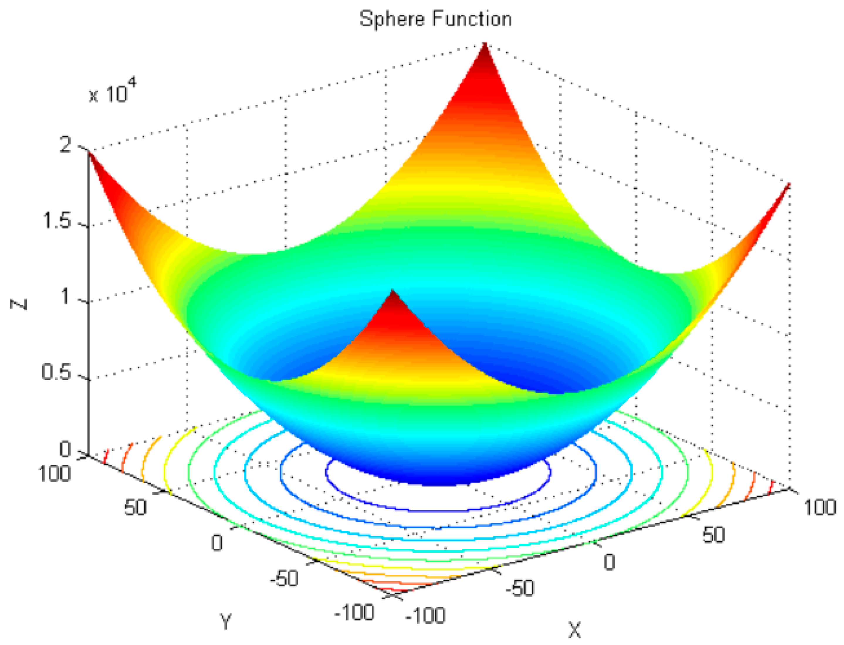
| Sphere | 30 | [0,0,…,0] | 0 | (−100,100) |
| Rosenbrock | 30 | [1,1,…,1] | 0 | (−2.048,2.048) |
| Griewank | 30 | [0,0,…,0] | 0 | (−8,8) |
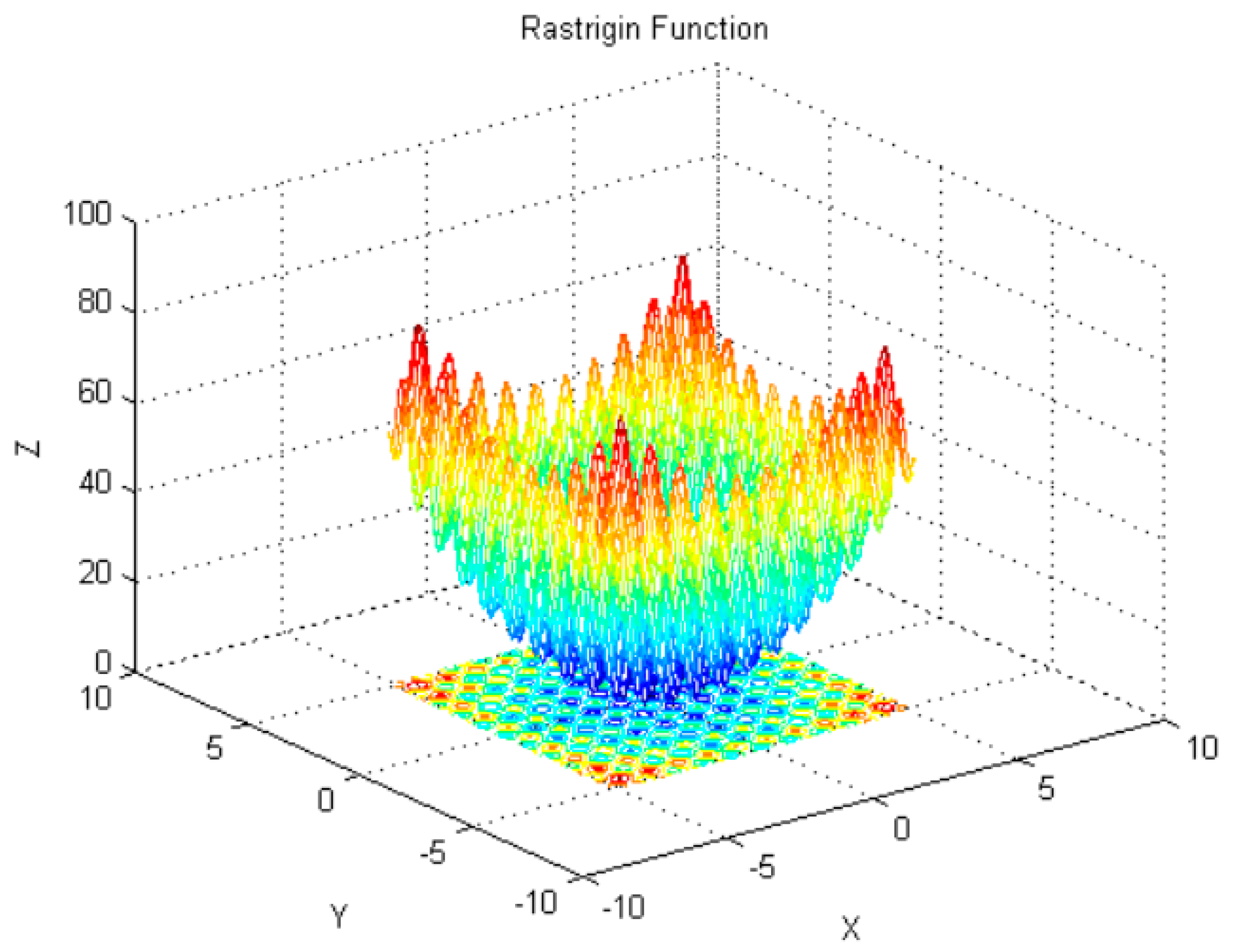
| Rastrigin | 30 | [0,0,…,0] | 0 | (−5.12,5.12) |
| Ackley | 30 | [0,0,…,0] | 0 | (−8,8) |
| Schwefel’s problem 22 | 30 | [0,0,…,0] | 0 | (−10,10) |
| Standard Function Type | PSO | FWA | CARLA | |||
|---|---|---|---|---|---|---|
| Mean Value | Standard Deviation | Mean Value | Standard Deviation | Mean Value | Standard Deviation | |
| Sphere | 0 | 0 | 0 | 0 | 0 | 0 |
| Rosenbrock | 66.59 | 204.29 | 12.16 | 12.82 | 8.91 | 10.22 |
| Griewank | 0 | 0.01 | 0 | 0 | 0 | 0 |
| Rastrigin | 6.77 | 7.70 | 0 | 0 | 0.01 | 0.21 |
| Ackley | 0.043 | 0.042 | 0 | 0 | 0 | 0 |
| Schwefel’s problem 22 | 23.93 | 13.61 | 0 | 0 | 0 | 0 |
| Wood-Berry | ||||
|---|---|---|---|---|
| Actual model | ||||
| Method in [26] (FRE) | ||||
| error (%) | 0.98 | 0.34 | 0.40 | 0.47 |
| Method in [20] (NPSO-FRE) | ||||
| error (%) | 0.32 | 0.014 | 0.015 | 0.024 |
| Method in [23] (MFA-FRE) | ||||
| error (%) | 0.32 | 0.004 | 0.008 | 0.005 |
| Method in this paper (CARLA-FRE) | ||||
| error (%) | 0.21 | 0.013 | 0.012 | 0.021 |
| Actual Model | Noise 0% | Noise 20% | ||
|---|---|---|---|---|
| MFA-FRE | CARLA-FRE | MFA-FRE | CARLA-FRE | |
| error (%) | 0.47 | 0.29 | 1.16 | 0.32 |
| error (%) | 0.75 | 0.39 | 6.45 | 0.65 |
| error (%) | 1.41 | 0.61 | 7.71 | 1.05 |
| error (%) | 0.92 | 0.47 | 3.02 | 0.91 |
| error (%) | 0.52 | 0.31 | 2.31 | 0.81 |
| error (%) | 0.24 | 0.25 | 2.75 | 0.79 |
| error (%) | 0.91 | 0.74 | 4.39 | 1.27 |
| error (%) | 2.70 | 0.55 | 2.70 | 2.06 |
| error (%) | 0.31 | 0.62 | 0.29 | 1.67 |
© 2019 by the authors. Licensee MDPI, Basel, Switzerland. This article is an open access article distributed under the terms and conditions of the Creative Commons Attribution (CC BY) license (http://creativecommons.org/licenses/by/4.0/).
Share and Cite
Jiang, M.; Jin, Q. Multivariable System Identification Method Based on Continuous Action Reinforcement Learning Automata. Processes 2019, 7, 546. https://doi.org/10.3390/pr7080546
Jiang M, Jin Q. Multivariable System Identification Method Based on Continuous Action Reinforcement Learning Automata. Processes. 2019; 7(8):546. https://doi.org/10.3390/pr7080546
Chicago/Turabian StyleJiang, Meiying, and Qibing Jin. 2019. "Multivariable System Identification Method Based on Continuous Action Reinforcement Learning Automata" Processes 7, no. 8: 546. https://doi.org/10.3390/pr7080546