Electromagnetic Hysteresis Based Dynamics Model of an Electromagnetically Controlled Torque Coupling

Abstract

This paper proposes a novel computationally efficient, easy-to-implement electromagnetic hysteresis based dynamics model of a kind of intelligent electromagnetic torque controlled coupling (EMTC), which, with drag torque under consideration, first models the electromagnetic hysteresis existing in the primary clutch with the classical Preisach model, and then models the transferred torques in the three friction elements of the center coupling in the slipping and locked modes, respectively. The performance of the model is verified by simulation and experiment jointly, which lays the basis for the development of advanced control algorithm.

1. Introduction

Although electric all-wheel drive vehicles have been a hot topic recently [1,2,3,4,5], the majority of the market share still vests in traditional mechanical AWD vehicles. The last few years have witnessed the evolution of the three generations of EMTC, the high fuel economy and excellent AWD performance make it widely used in many AWD cars, see Figure 1. Controlling of the AWD vehicles has attracted much attention of researchers [6,7,8,9,10], however, a solid and effective model of the AWD effecter remains critical. To address that issue, a lot of literatures have been focused on modeling EMTC along the years.

Torii [11] simply proposed the modeling method of an electronically controlled torque-splitting multi-plate clutch, which is the prototype of today’s EMTC. Mohan [12] made an attempt to incorporate the four-wheel drive and AWD systems and their driveline architectures, and to explain the control tactics and philosophies behind the controlling of these traction systems. Cheli [13] introduced a type of driveline torque distribution management device with the corresponding control strategy, which was verified by using a precise vehicle model developed in Simulink. Lee [14] proposed a control system design method for a 4WD vehicle that distributed the front and rear driving torques through a clutchless center limited slip differential, the control system consisted of a control map with three different control modes and vehicle steering estimation method. Piyabongkarn [15] proposed a modeling method for the center coupling and the electronically controlled limited slip differential (ELSD), the controlling of which was designed in hierarchical architecture. Ando [16] came up with two 3D maps to describe the relations between vehicle speed, clutch opening, front-rear wheel speed difference and the driving torque output by EMTC which is quite implementable in the controller. In [17] the advantage of high efficiency of BorgWarner NexTrac^TM was introduced, with new friction plate materials and innovatively compact layout, the newly released NexTracTM was capable of transferring larger driving torque with smaller configuration. Vantsevich [18] presented a hypothetical driveline power-dividing unit with the modeling method, the control algorithm of which allowed for flexible controlling of the power flow to the drive wheels.

The EMTC modeled in this paper consists of three friction elements that are conditioned and lubricated by viscous fluid or oil, namely, the EMTC is a wet clutch internally. To model the wet clutch, various researches and modeling methods have been proposed. Ando [19] described the third generation of electronically controlled AWD coupling that contributed higher fuel efficiency by reducing the drag torque due to the viscosity of the lubricant while the clutches were not engaged. Iqbal et al. [20] presented a mathematical model for the estimation of drag torque in multi-disk wet clutches considering the laminar flow in the clearance between the friction disks, and the simulation results validated the model’s capability of predicting the drag torque in higher clutch speed range. Völkel [21] investigated the influences of such factors as oil flow rate and design of grooves on the cooling properties and thermal behavior of the wet multi-disk clutches, the flow capacity determinations were also presented, and the scoop grooves conveying effect was finally explained.

Despite the various researches on the modeling of the electronically or electromagnetically controlled center coupling, some key factors that can influence the driving torque governed by EMTC greatly, such as the hysteresis in the electromagnet and the torque allocation in the three friction elements, haven not been taken into consideration or discussed in detail [22], and a more explicit way of dynamically modeling the three friction elements is still missing. Thus, to accurately control the driving torque transferred by EMTC, these issues will be addressed in this paper.

This paper is organized in three parts: First, the electromagnetic force generated by the primary clutch apply system (coil and armature) is modeled utilizing the Preisach model in the environment of Matlab/Simulink; then, the central clutch status will be decided between ‘slipping’ and ‘locked’ modes based on the vehicle states detected by sensors, and the driving torques transferred in condition of the two modes will be calculated; and finally, the model built in this paper will be verified through a real-car experiment regarding the slipping and locked modes.

2. Electromagnetic Force Modeling

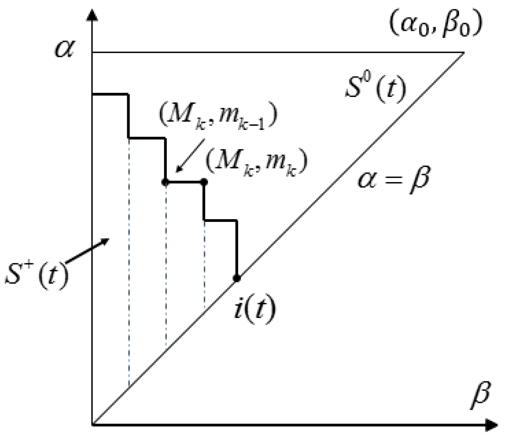
2.1. Hysteresis Modeling

The effect of magnetic hysteresis in the electromagnet materials is crucial in predicting the magnetic compression force generated. To model the magnetic hysteresis phenomenon presented in ferromagnetic materials, various modeling methods have been developed. For the electromagnet in EMTC, which is made of soft magnetic materials, the Preisach model is suitable to be implemented using the numerical implementation method mentioned in [23,24]. The electromagnetic force depends on the input current and the airgap between the electromagnet and the armature, whereas the hysteresis effect of the airgap is negligible, then for the general current input trajectory, the output values are as follows:

$$f(t)=\Gamma u(t)={\displaystyle \iint \mu (\alpha ,\beta ,h(t))}{\widehat{\gamma }}_{\alpha \beta }u(t)\mathrm{d}\alpha \mathrm{d}\beta$$

(1)

$$f(t)={\displaystyle \sum _{k=1}^{n-1}(f_{M_k{m}_k}-f_{M_k{m}_{k-1}})+f_{M_{n}u(t)}-f_{M_n{m}_{n-1}}}$$

(2)

$$f(t)={\displaystyle \sum _{k=1}^{n-1}(f_{M_k{m}_k}-f_{M_k{m}_{k-1}})+f_{u(t)}-f_{u(t)m_{n-1}}}$$

(3)

In Equation (1), ${\widehat{\gamma }}_{\alpha \beta }u(t)=0,\forall (\alpha ,\beta )\in S^o(t)$, ${\widehat{\gamma }}_{\alpha \beta }u(t)=1,\forall (\alpha ,\beta )\in S^{+}(t)$, the areas denoted by $S^o(t)$ and $S^{+}(t)$ can be found in Figure 2, $\alpha ,\beta$ represent the ascending and descending value of the input current in each instant of time, respectively. Equations (2) and (3) calculate the output values in condition of decreasing and increasing input respectively. In the equations, $f_{u(t)}$ denotes the output value on the limiting ascending branch corresponding to the input value $u=u(t)$, in which $u(t)$ is the current time input value; $M_i$, $m_j$ indicate the global maximum and minimum inputs of each instant of time, respectively; $f_{M_i{m}_j}$ corresponds to the output value at $\beta =m_j$ that lies on the first-order transition curve attached to the limiting ascending branch at the point $\alpha =M_i$.

Using the method mentioned in [25], as the limit working currents of the electromagnet are ${\alpha }_0={\beta }_0=4.5\mathrm{A}$, the triangle T containing a grid of points is devised, the intervals between two adjacent points are expressed as $\Delta \alpha =\Delta \beta =0.5\mathrm{A}$. The experimental settings are shown in Figure 2, the forces are measured with an FCS system (manufactured by Beijing FCS Corp.) containing a force sensor, which is mounted on the ferromagnetic armature. The airgap between the armature and the electromagnet can be varied by controlling the up and down movement of the shaft. Using that experimental setting, the forces at each point of inside the triangle T, see Figure 3, can be determined.

For every instant of time, the extrema of the input will be updated, and the output will be calculated. If the input current doesn’t lie at the grid point of the triangle, the following interpolation equations can be applied [25]:

$$f_{\alpha \beta }=C_0+C_1\alpha +C_2\beta +C_3\alpha \beta$$

(4)

if the input current extrema ($M_n{m}_n$) belongs to a square cell. And if the extrema lie in a triangular cell that is adjacent to the line $\alpha =\beta$,

$$f_{\alpha \beta }=C_0+C_1\alpha +C_2\beta$$

(5)

where $C_i$ can be acquired by matching the values of $f_{\alpha \beta }$ in the cell vertices.

As for the effect of airgap, which changes from 0.2 mm to 1.4 mm, on the electromagnetic force, seven calibration points with the step of 0.2 mm are selected, and the electromagnetic forces along the general current trajectory at each point are measured as in the triangle gridding mentioned above. Then the force output at a certain airgap that doesn’t lie at the gridding point, can be calculated with the method of second-order polynomial interpolation.

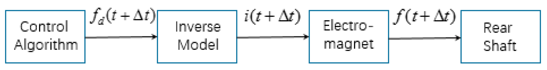
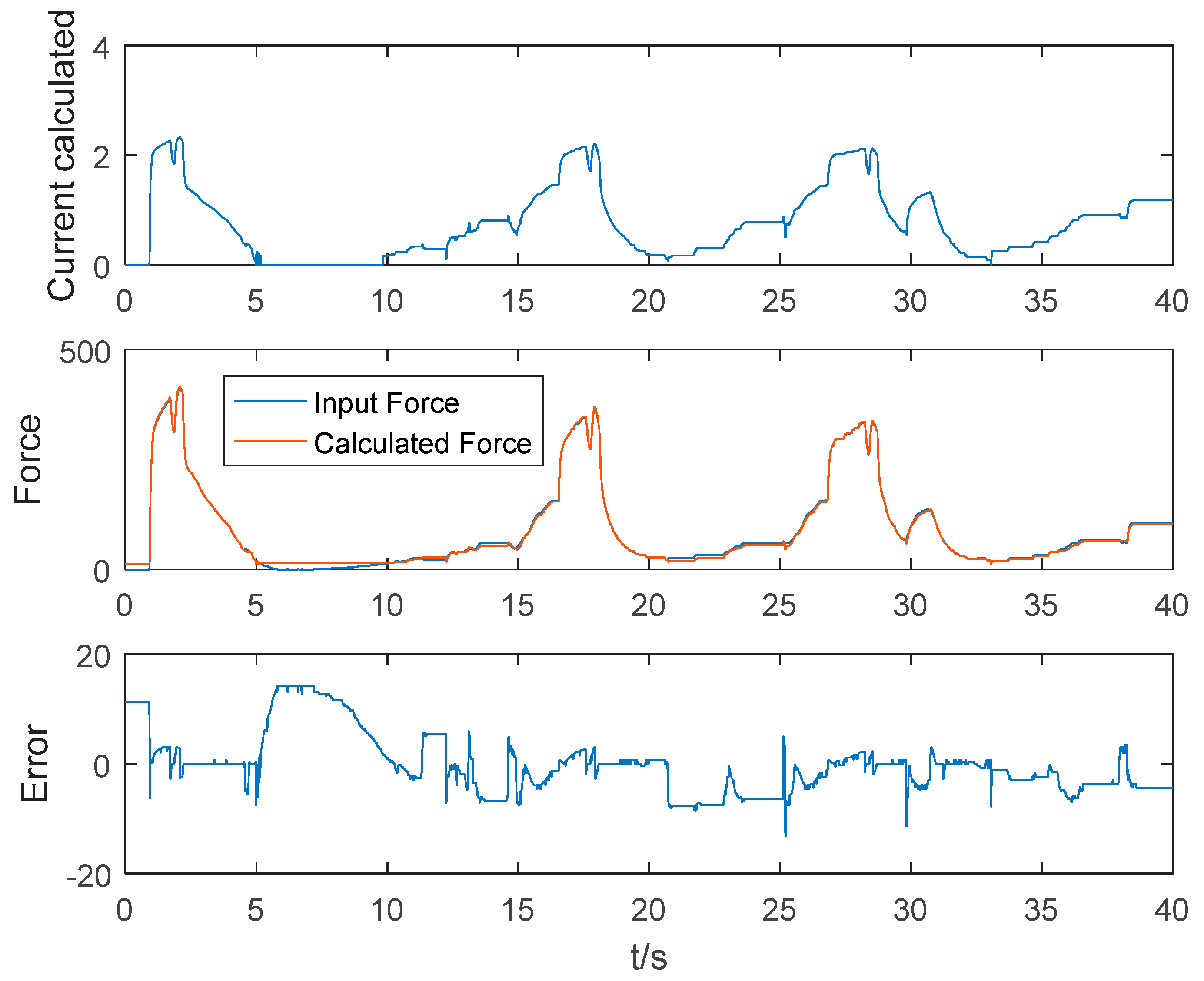
2.2. Verification and Inverse Compensation of Hysteresis Model

To verify the effectiveness and validity of the hysteresis model, the electromagnet set in the primary clutch of EMTC is measured for output electromagnetic force with input current. The current in the coil was energized by linear power supply in a range of 0–4.5 A, and the magnetic forces were measured utilizing a torque sensor mounted on the armature. With the experimentally acquired data, as shown in Figure 4, the hysteresis model can be established. The comparison results are shown as follows.

In Figure 5, the performance of the proposed model in normal scenario, where the amplitude of the current input first decreases then increases, proves the effectiveness and accuracy in predicting the corresponding force output with respect to the current input. While in Figure 6, the result shows the effective prediction performance when the airgap doesn’t lie at the gridding point. Now it’s possible to design an inverse controller to offset the hysteresis effects and increase the accuracy of the electromagnetic force commanded.

Based on the theories and formulas in [25],

$$\{\begin{array}{l}{f}_d(t+\Delta t)={\displaystyle \sum _{k=1}^l(f_{M_k{m}_k}-f_{M_k{m}_{k-1}})+G_{M_{l+1}u(t+\Delta t)}-f_{M_{l+1}{m}_l}}\\ i(t+\Delta t)=\beta =G^{-1}(-{\displaystyle \sum _{k=1}^l(f_{M_k{m}_k}-f_{M_k{m}_{k-1}})}+f_{M_{l+1}{m}_l}+f_d(t+\Delta t))\end{array}$$

(6)

the corresponding current in the case of decreasing target force output, $m_l<\beta =i(t+\Delta t)<m_{l+1}$, can be acquired, and for increasing force output, $M_{l+1}<\alpha =i(t+\Delta t)<M_l$, the corresponding input current can be obtained by the follows equations:

$$\{\begin{array}{l}{f}_d(t+\Delta t)={\displaystyle \sum _{k=1}^l(f_{M_k{m}_k}-f_{M_k{m}_{k-1}})+f_{u(t+\Delta t)}-f_{u(t+\Delta t)m_l}}\\ G(t+\Delta t)=f_{u(t+\Delta t)}-f_{u(t+\Delta t)m_l}\\ i(t+\Delta t)=\alpha =G^{-1}(f_d(t+\Delta t)-{\displaystyle \sum _{k=1}^l(f_{M_k{m}_k}-f_{M_k{m}_{k-1}})})\end{array}$$

(7)

Upon obtaining the accurate compensation current to be input in the next instant of time, an open-loop compensation of electromagnetic hysteresis can be devised to achieve the desired output profile, as in Figure 7.

The verification of the performance of the inverse model can be conducted by comparing the output of the electromagnet and the input calculated force that can also be seen as the output of some anhysteretic material. The comparison of the measured data and the input to the model can be seen in Figure 8.

As is shown in the figure, there are some minor errors detected between the reference values and the measured values. The main possible error sources can be measurement error, interpolation error of the model and computational delay, which tend to be easily eradicated by increasing the number of reference points in the Preisach triangle. For this reason, it is safe to say that the output corresponding to the current input converted follows excellently the target force generated by the control algorithm.

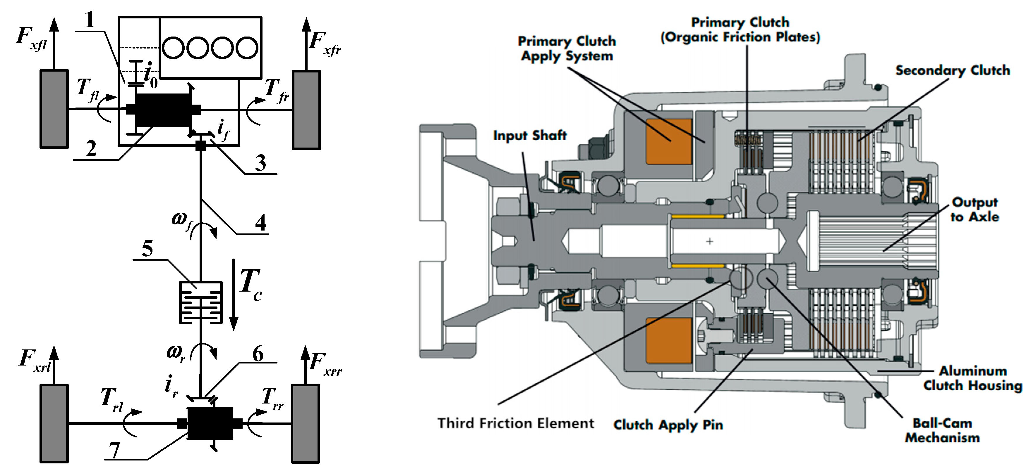
3. EMTC Dynamics Model

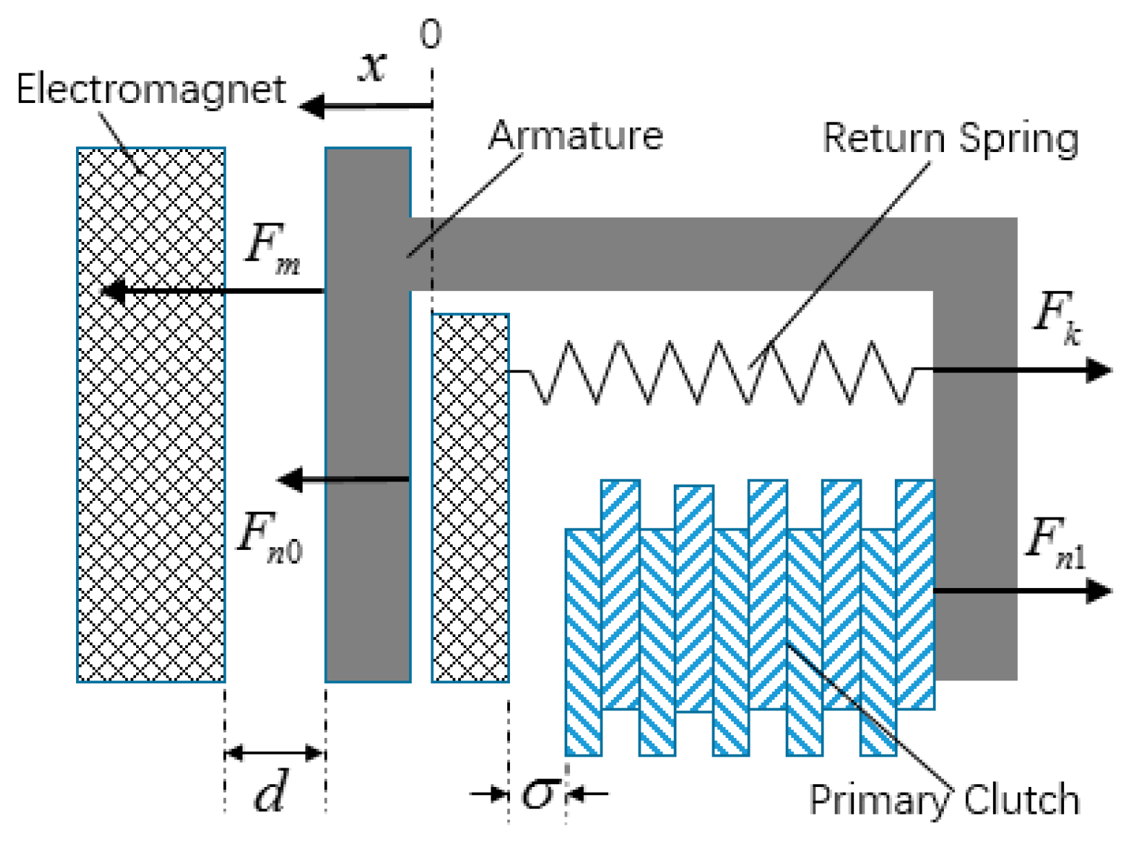
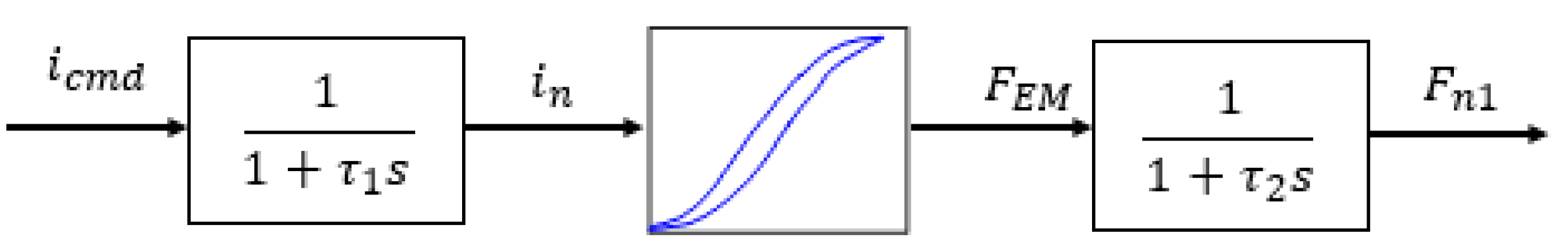
3.1. The Electromagnetic Actuator Model

The schematic diagram of the electromagnetic effector is illustrated as follows in Figure 9 [26]:

Set $K_{spring}$ as the stiffness of the spring, $F_{k0}$ the original spring force, $c_{spring}$ the spring damping and $m_0$ the mass of the armature. Then the dynamics equation of the electromagnetic effector can be expressed as follows:

$$F_m+F_{n0}-F_{n1}-F_k-c_{spring}\cdot \dot{x}=m_0\cdot \ddot{x}$$

(8)

Namely,

$$F_m+F_{n0}-F_{n1}-K_{spring}\cdot x-F_{k0}-c_{spring}\cdot \dot{x}=m_0\cdot \ddot{x},x\in [0,\sigma ]$$

(9)

where,

$$F_{n0}=\{\begin{array}{ll}{F}_{k0}-F_m& x=0\\ 0& x\ne 0\end{array},x\in [0,\sigma ]$$

(10)

$$F_{n1}=\{\begin{array}{ll}{F}_m-F_{k0}-K_{spring}\sigma & x=\sigma \\ 0& x\ne \sigma \end{array}$$

(11)

and the airgap can be expressed as:

$$\delta =d-x,(d>\sigma \ge x)$$

(12)

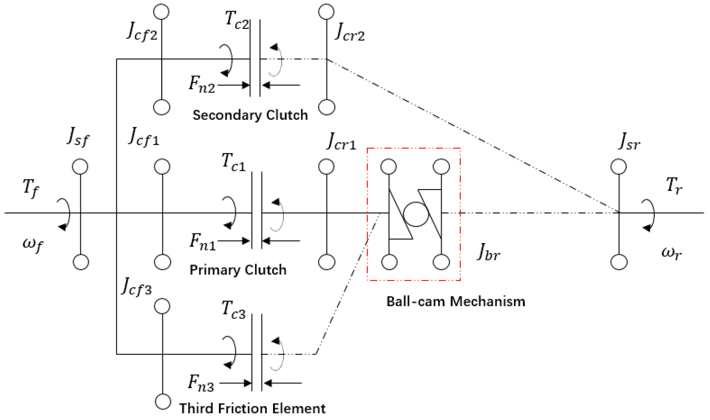
3.2. The Torque Transfer Model

The two clutches and the third friction element can work in two different modes apart from the ‘separated’ mode, like other kinds of clutches, slipping and locked modes. The fact that the torques transferred in these two modes are different even with other conditions remaining the same, makes the precise modeling of the torque transmitting process of great significance [26].

The driving plate of the primary clutch is connected to the housing of the input shaft (interference fit with the input shaft), the engaged plate to the ball-cam mechanism by spline connection, the driving cam of which is then connected to the output shaft by spline, thus, under the static and quasi-static circumstances, there is no rotational speed difference between the driving and engaged plates of the ball-cam mechanism, which in turn leads to the equality of the speeds of the engaged plate of the primary clutch and the output shaft. The driving and engaged plates of the secondary clutch are inner and outer spline-connected to the housing of the input shaft and the output shaft, respectively. And the driving plate of the third friction element is fixed on the input shaft, the engaged plate to the driving plate of the ball-cam mechanism. In a nutshell, the three friction elements are zero-speed-differently connected to the input and output shafts at the both ends of them, the whole system can be seen as a parallel structure, while the primary clutch and the third element comply to series connection of the output ends at the ball-cam mechanism.

The layout of the three torque transfer elements is shown in Figure 10.

The modes transition strategy is determined in Figure 11 [26]. As regards the slipping mode, with the increase of the compression force of the electromagnet, the locking mode steps in if the torque capacity of the clutch $T_{cap}$ exceeds the torque required when being locked $T_{lock}$, and it only happens when the speed difference fades gradually to zero. One thing worth mentioning is that, generally during the mode transition, shock occurs because of the sharp change of the torque transferred, as the static friction coefficient is slightly larger than that of the slipping friction, which is also an essential factor that should be taken into consideration in the control algorithm.

Based on the empirical values, it is also plausible to set $1.02\cdot T_{cap}<T_{lock}$ as the threshold of the clutch’s transition into slipping mode, as is illustrated in Figure 10, where, according to Newton’s Law, $F_{n2}=F_{n3}$, $\Delta \omega ={\omega }_f-{\omega }_r$, $\Delta {\omega }_{pre}$ is the speed difference of the last step, $T_{cap\_S}$ is the torque capacity of the clutch in slipping mode, and $T_{cap\_L}$ is the torque capacity in lock mode.

3.2.1. Torque Transfer Model for Slipping Mode

In condition of slipping mode, the torques $T_{ci}(i=1,2,3)$ transferred by the three friction elements are kinetic friction torques $T_{ki}$ that can be calculated as follows:

$$\{\begin{array}{l}{T}_{c1,2}=T_{k1,2}=\frac{2}{3}{\mu }_{k1,2}{R}_{1,2}{F}_{n1,2}{z}_{1,2}\\ T_{c3}=T_{k3}=\frac{2}{3}{\mu }_{k3}{R}_3{F}_{n2}\end{array}$$

(13)

where, ${\mu }_{ki}$ are the kinetic friction coefficients of the primary, secondary clutch and the third friction element, respectively, $F_{n1},F_{n2}$ are the compression force applied on the primary and secondary clutches, $z_1,z_1$ are the number of friction pairs of the two clutches, and $R_i$ are the effective radiuses of the three elements.

Neglect the moment of inertia of the driving plate in the ball-cam mechanism, the compression force applied on the secondary clutch and the third friction element is,

$$F_{n2}=\frac{\lambda }{R}{T}_{in}=\frac{\lambda }{R}(T_{k1}+T_{k3})$$

(14)

In the equation above, $T_{in}$ is the torque transferred by the ball-cam mechanism, $R$ is the working radius of the mechanism, and $\lambda$ is the amplifier ratio of the mechanism that can be measured experimentally and seen as a constant.

Substituting those formulae, the torques transferred and torque capacities of each friction element can be obtained:

$$\{\begin{array}{l}{T}_{c1}=T_{k1}=\frac{2}{3}{\mu }_{k1}{R}_1{F}_{n1}{z}_1\mathrm{sgn}(\Delta \omega )\\ T_{c2}=T_{k2}=\frac{2\lambda {\mu }_{k2}{R}_2{z}_2}{3R-2\lambda {\mu }_{k3}{R}_3}{T}_{k1}\\ T_{c3}=T_{k3}=\frac{2\lambda {\mu }_{k3}{R}_3}{3R-2\lambda {\mu }_{k3}{R}_3}{T}_{k1}\end{array}$$

(15)

$$T_{cap\_Si}=\frac{{\mu }_{si}}{{\mu }_{ki}}{T}_{ki}$$

(16)

where ${\mu }_{si}$ denotes the kinetic friction coefficients of the primary, secondary clutch and the third friction element, respectively.

Thus, the total torque transferred and the torque capacity are,

$$T_c={\displaystyle \sum _{i=1}^3{T}_{ci},T_{cap\_S}={\displaystyle \sum _{i=1}^3{T}_{cap\_Si}}}$$

(17)

3.2.2. Torque Transfer Model for Locked Mode

When the clutches are locked in the sense of speed, the static friction torques transferred $T_{li}$ can vary and shift among the three friction elements with the total torque changing, considering the parallel structure of the clutches shown in previous sections. The torque distribution of the three friction elements can be divided into three conditions, as illustrated in Figure 12.

In Figure 11, the distribution is shown as an example under the circumstances of $T_{cap1}>T_{cap3}$, while the contrary condition also stands a chance in the real car. To explain the distributions in detail, we set $T_{li},T_{cap\_li}$ as the static friction torque and the torque capacity in locked mode for the primary clutch, the secondary clutch and the third friction element, respectively.

• The torque transferred is small enough for the three elements to divide equally:

  $$\{\begin{array}{c}{T}_{li}=\frac{T_{lock}}{3}\\ T_{cap\_l1,2}=\frac{2}{3}{\mu }_{s1,2}{R}_{1,2}{z}_{1,2}{F}_{n1,2},T_{cap\_l3}=\frac{2}{3}{\mu }_{s3}{R}_3{F}_{n2}\\ F_{n2}=\frac{\lambda }{R}(T_{l1}+T_{l3})\end{array}$$

  (18)
• The capacity of the third element, $T_{cap\_l3}$, passes through as it doesn’t exceed $T_{lock}/3$, and the rest will be taken over by the other two clutches:

  $$\{\begin{array}{c}{T}_{l3}=T_{cap\_l3}=\frac{\lambda {\mu }_{s3}{R}_3{T}_{lock}}{3R-\lambda {\mu }_{s3}{R}_3},T_{l1}=T_{l2}=\frac{T_{lock}-T_{l3}}{2}\\ T_{cap\_l1,2}=\frac{2}{3}{\mu }_{s1,2}{R}_{1,2}{z}_{1,2}{F}_{n1,2}\end{array}$$

  (19)
• The primary clutch and the third friction element both transmit the maximum of them, and the secondary clutch takes care of the rest:

  $$\{\begin{array}{c}{T}_{l1}=T_{cap\_l1}=\frac{2}{3}{\mu }_{s1}{R}_1{z}_1{F}_{n1},T_{l2}=T_{lock}-T_{l3}-T_{l1}\\ T_{l3}=T_{cap\_l3}=\frac{2\lambda {\mu }_{s3}{R}_3}{3R-2\lambda {\mu }_{s3}{R}_3}{T}_{cap\_l1}\\ T_{cap\_l2}=\frac{2\lambda {\mu }_{s2}{R}_2{z}_2}{3R-2\lambda {\mu }_{s3}{R}_3}{T}_{cap\_l1}\end{array}$$

  (20)

In condition of $T_{cap1}>T_{cap3}$, a switch of $T_{l1}$ and $T_{l3}$ will meet the requirement and the equations are quite similar to those listed above. The total torque transferred and the total torque capacity are:

$$T_c={\displaystyle \sum _{i=1}^3{T}_{li}=T_{lock},T_{cap\_L}=}{\displaystyle \sum _{i=1}^3{T}_{cap\_li}}$$

(21)

Based on the previous discussions, the torque distribution logic can be devised.

3.3. Friction and Drag Torque Model

The friction coefficient between two friction discs can vary due to the variation of the factors such as the temperature inside the clutches. Modeling the friction situation is a challenging task. Despite the difference of the friction types, the Lugre model has made it possible to unify the representation of these types in one formula [27], in which the friction coefficient is the function of the bristle deflection $z$ and the speed difference between the friction surfaces $v$.

$$\mu ={\sigma }_{0}z+{\sigma }_1\dot{z}+{\sigma }_{2}v$$

(22)

$$\dot{z}=v-{\sigma }_0\frac{\left|v\right|}{g(v)}z$$

(23)

$$g(v)={\mu }_{cl}+({\mu }_p-{\mu }_{cl})e^{-{(v/v_s)}^2}$$

(24)

where, ${\sigma }_0$ and ${\sigma }_1$ are the tangential direction stiffness and damping coefficient, ${\sigma }_2$ the viscous friction coefficient, ${\mu }_c$ the Coulomb friction coefficient, ${\mu }_p$ the peak friction coefficient, and $v_s$ the Stribeck velocity. The six parameters are typically bristle-related, and therefore can be experimentally determined. Then the static and kinetic friction coefficients can both be identified with varied speed difference between the friction surfaces.

It was discovered in experiments that there is torque transferred in the clutches even in disengaged phases. This uncontrollable and undesired torque is defined as drag torque, which is induced by the resistance of the lubricant fluid filled in the clutches to the relative rotation of the friction discs. The factors that influence the drag torque of the multi-plate clutch include the number of discs, the clearance between two consecutive discs, lubricant flow rate, internal temperature of the clutch and the radius of the friction discs.

The calculation of drag torque can be expressed as follows,

$$T_{drag}=\frac{N\pi \omega \mu }{2h}(R_o^4-R_1^4)$$

(25)

where, $N$ denotes the number of friction pairs, $\mu$ the dynamic viscosity of the clutch fluid, $\omega$ the relative rotational speed of the clutch discs, $h$ the axial clearance between two consecutive discs, $R_o$ the equivalent radius and $R_1$ inner radius of the discs. The detailed parameter selection and calculation were given in [28]. And the drag torque variation with respect to the relative rotation speed is shown as s in Figure 13.

Then the overall driving torque the EMTC transfers is expressed as,

$$T_{all}=\{\begin{array}{l}{T}_{drag},\eta =0\\ T_c,\eta =1\end{array}$$

(26)

where, $\eta =0$ denotes the clutch is in disengaged mode, and $\eta =1$ means the clutch is engaged.

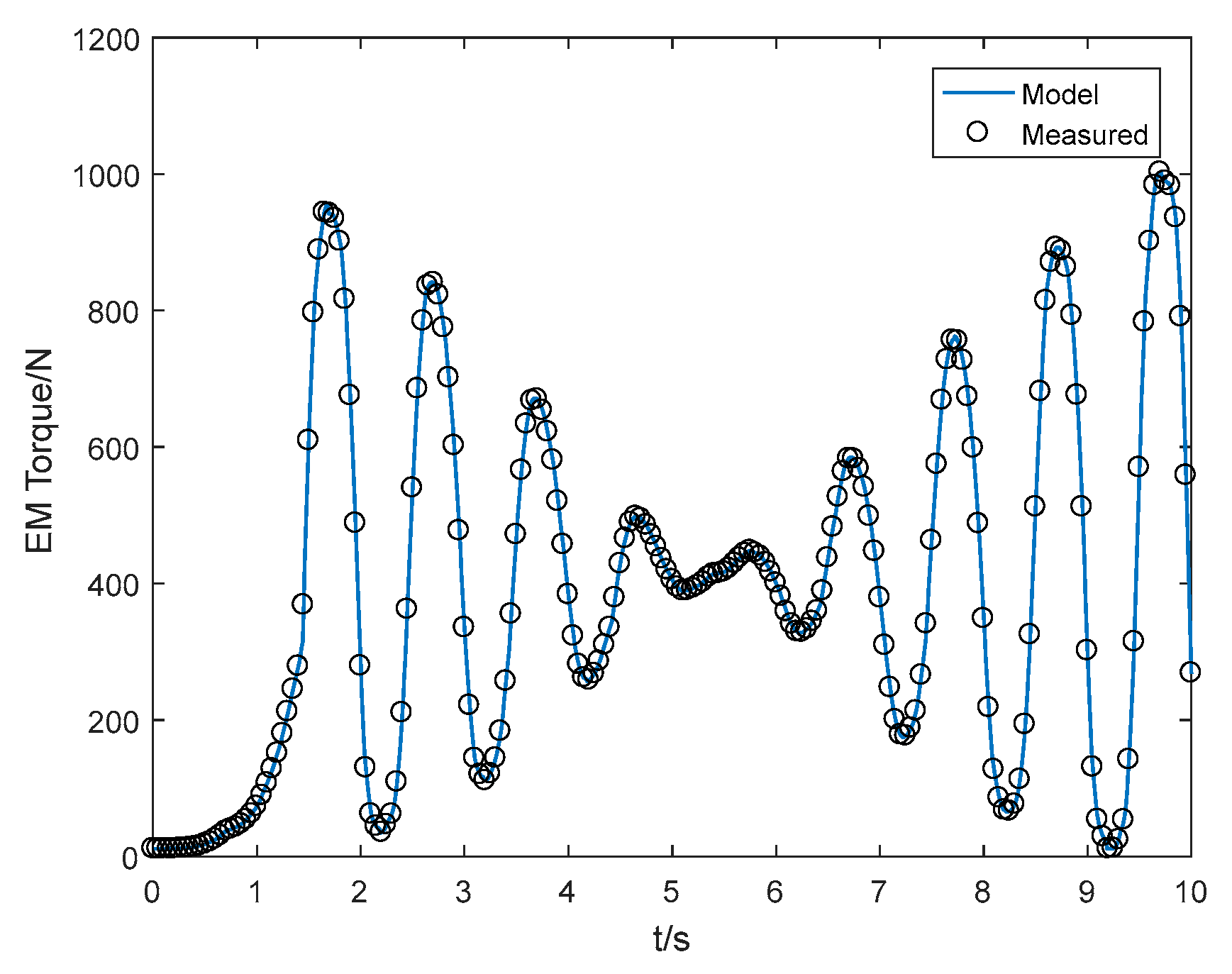
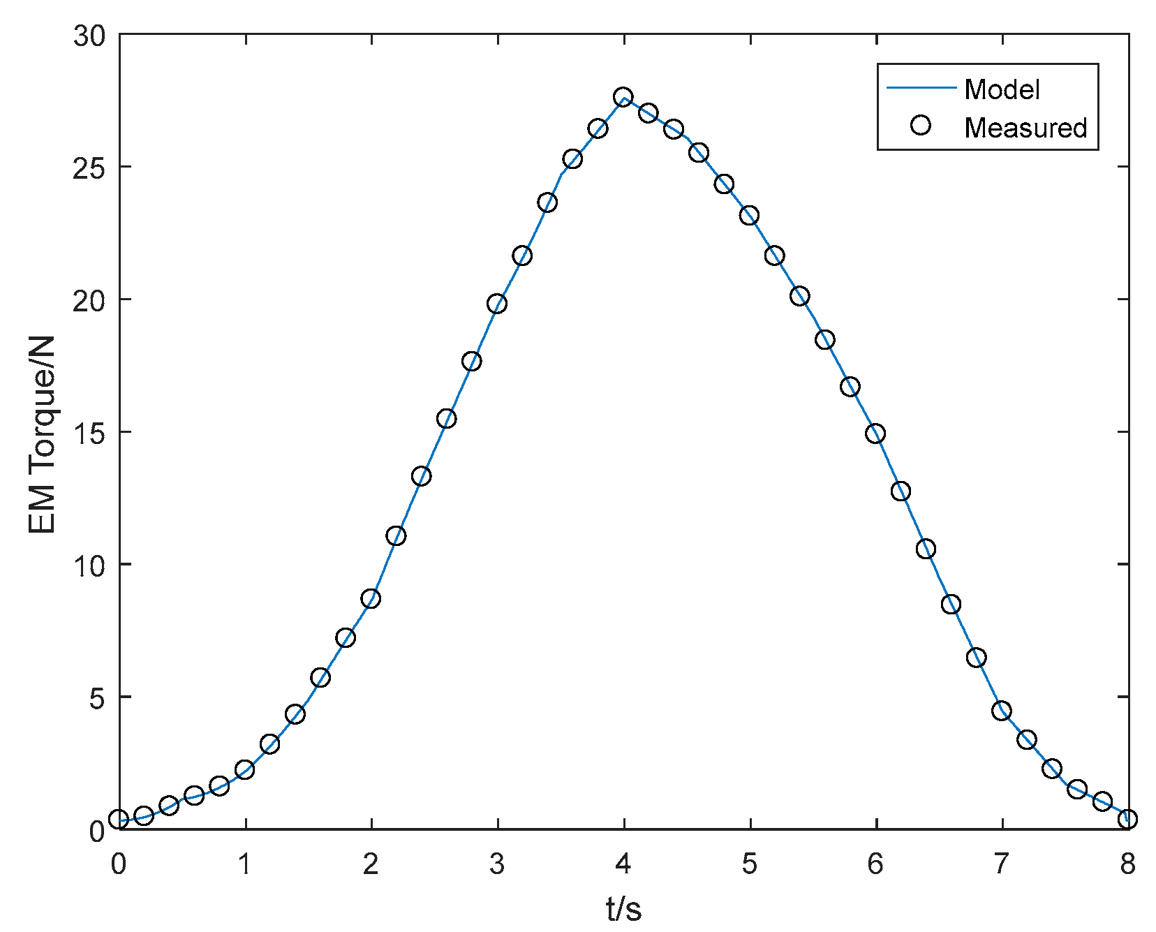
4. Experimental Verification of the Dynamic Model

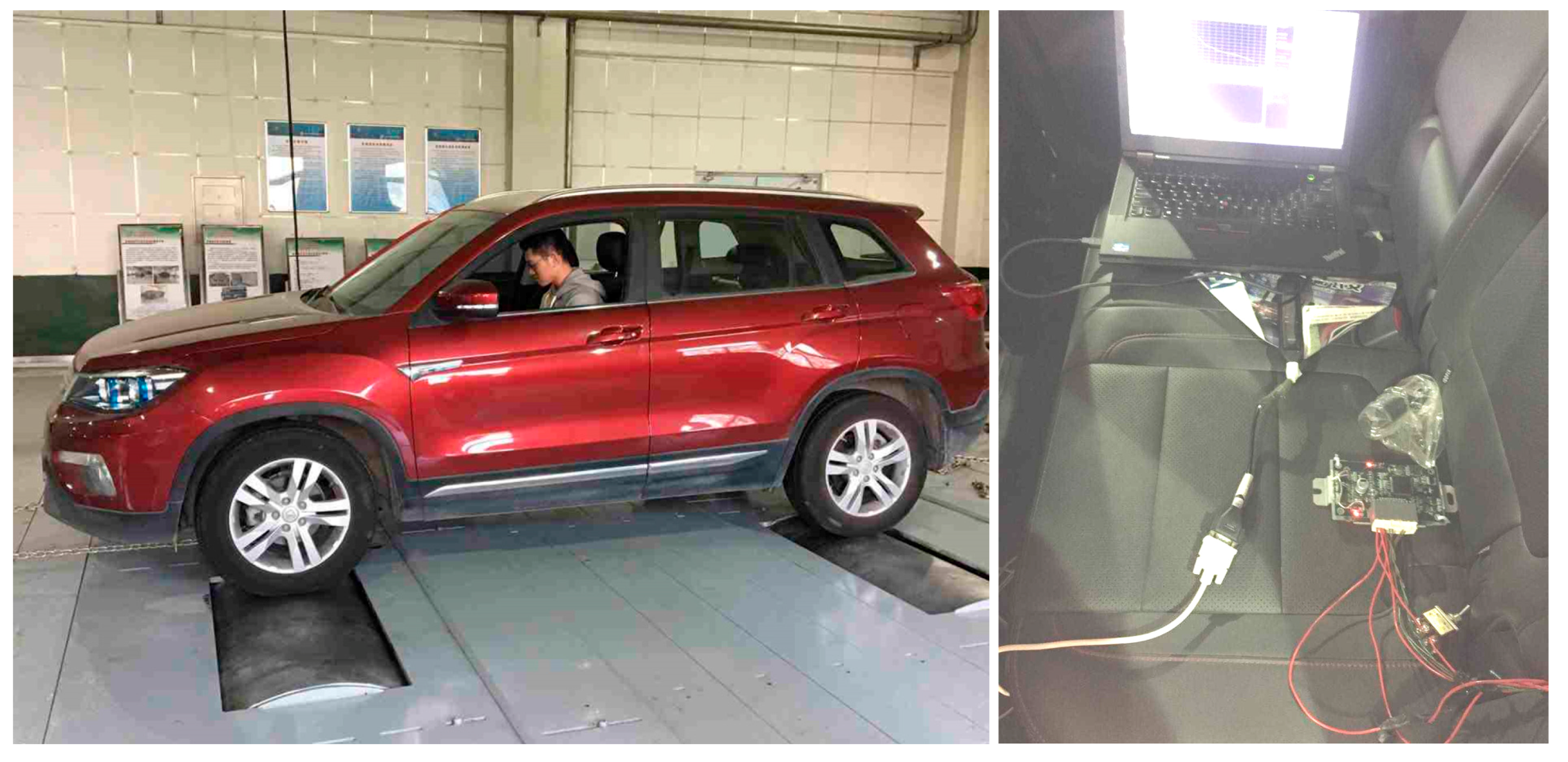
4.1. The Experiment Settings

When the EMTC model is connected with a whole-car model, the transferred lock torque $T_{lock}$ will be decided by the driving torque input from the engine and the road condition jointly. Then according to Figure 1,

$$\begin{array}{l}{T}_{trans}{i}_0-T_{cf}{i}_f-{\displaystyle \sum F_{xf}r-{\displaystyle \sum T_{ff}}}=J_{wf}(\frac{{\dot{\omega }}_{cf}}{i_f})\\ T_{cr}{i}_r-{\displaystyle \sum F_{xr}}r-{\displaystyle \sum T_{fr}=J_{wr}}(\frac{{\dot{\omega }}_{cr}}{i_r})\\ T_{cf}-T_{lock}=J_{sf}{\dot{\omega }}_{cf}\\ T_{lock}-T_{cr}=J_{sr}{\dot{\omega }}_{cr}\end{array}$$

(27)

where, $J_{wf},J_{wr}$ are the net integrated moments of inertia of the front and rear drive axle and the wheels, respectively; $J_{sf},J_{sr}$ are the moment of inertia of the driving and engaged shaft of the EMTC; $T_{trans}$ is the output torque of the transmission and $i_0$ the gear ratio for the front retarder; $T_{cf},T_{cr}$ and ${\omega }_{cf},{\omega }_{cr}$ denote the rotational speed and driving torques of the input and output shaft of the EMTC, respectively; $T_{ff},T_{fr}$ indicate the rolling resistance torques originated from the revolving drums and exerted on the front and rear wheels.

To assure the performance of the locked mode, the gear ratios of the front and rear axles against the center coupling should be equal,

$$i_f=i_r$$

(28)

Substituting (28) into (27), we get

$$\{\begin{array}{l}{T}_{lock}=\frac{J_r{i}_0{T}_{trans}-r(J_r{\displaystyle \sum F_{xf}-J_f{\displaystyle \sum F_{xr}}})-(J_r{\displaystyle \sum T_{ff}-J_f{\displaystyle \sum T_{fr}}})}{i_{inter}(J_f+J_r)}\\ \mathrm{where},J_f=J_{sf}+\frac{J_{wf}}{i_{inter}^2}{J}_r=J_{sr}+\frac{J_{wr}}{i_{inter}^2}\end{array}$$

(29)

And to improve the robustness and the practicability of the model, a Torsen reversal damping model is added to the output lock torque,

$$\begin{array}{l}{T}_{lock}^{’}=T_{lock}+T_{Torsen}\\ T_{Torsen}=K_s{\displaystyle \int ({\omega }_{cf}-{\omega }_{cr})}dt+D_s({\omega }_{cf}-{\omega }_{cr})\end{array}$$

(30)

where, $K_s,D_s$ denote the equivalent stiffness and damping coefficient of the driving system.

To give a reference for the input current of the EMTC, a two-input control algorithm of estimated output torque is designed,

$$T_{cal}(t)=f(thr(t),v_x(t))$$

(31)

where $T_{cal}(t)$ is the calculated reference value of the transferred torque by EMTC, $thr$ indicates the throttle opening, and $v_x$ denotes the vehicle longitudinal velocity.

The calculated value and the measured value in the experiment will be compared to verify the effectiveness of the dynamic model.

4.2. Real-Car Experiment

The car used in this experiment is an FWD (front-wheel driving) based real-time AWD sport utility vehicle, the system configuration is as shown in Figure 1, and the main parameters are listed in

Table 1. Main parameters of the prototype car.

Type	Unit	Value
Curb Weight	kg	2162
CM to front axle	mm	1104.3
CM to rear axle	mm	1595.7
Height of center of mass	mm	670
Wheel base	mm	2700
Transmission gear ratio	-	(1st)4.044/(2nd)2.371/(3rd)1.556/(4th)1.159/(5th)0.852/(6th)0.672/(R)3.19
Front main retarder ratio	-	3.75
Rear main retarder ratio	-	2.533
Engine power	kw	125
Tyre size	-	225/65R17

.

The real-car experiment is conducted on a Mustang revolving drum test table, see Figure 14, which consists of eight pairs of independent revolving drums and one control system, it is able to adjust both the rotating speeds and resistant torques of the drums while measuring the driving torques working on them. In order to test the output torque of the EMTC in slipping and locking modes, the speed differences of the two axles can be set to a considerable positive constant and some value close to zero, respectively.

To eliminate the spikes and some unknown perturbations [9], two first-order responses (${\tau }_1,{\tau }_2$) are implemented for the control of the current [10], as shown in Figure 15.

Then the test results for slipping and locked modes are illustrated in Figure 16 and Figure 17, respectively.

Figure 16 shows the states of the vehicle and the torques transferred in condition of slipping mode. It can be seen that the difference between the front and rear wheel speeds almost remained constant throughout the experiment time; The transferred torques in each of the three elements are proportional to the overall transferred torque, and the calculated torque from the model matches excellently the measured torque to a large extent; Figure 17 denotes those states and torques in condition of locked mode, in which the torques transferred in the three friction elements display the three situations depicted in the chapter above, and the calculated torque follows the measured values precisely. The effectiveness of the dynamic model can be verified through all those results together.

5. Conclusions and Future Work

An EMTC dynamics model has been developed considering the electromagnetic hysteresis effect in the primary clutch and the torque distribution when the clutches are in disengaged, locked and slipping modes, respectively, which lays the groundwork for advanced control algorithm for EMTC. The simulation and experiment results verified the validity and effectiveness of the model.

The contributions of this paper can be summarized into two points: First, the model proposed in this paper takes the electromagnetic hysteresis into consideration, which can have a significant effect on the accuracy of the calculation of the output driving torque; and second, three working modes of EMTC are classified and the corresponding driving torques calculation is given mathematically.

As an important part of the fail-safe system, the thermal factor of the clutches is essential to the control effectiveness of the EMTC, especially in the trapped situation. Thus, the thermal model of EMTC is also worth investigating. In addition, advanced control strategies based on mechanical 4WD system aiming at improving the mobility and stability of the vehicle are essential for the development of a complete 4WD system, all of which will be discussed in later literature.

References

1. Wu, D.M.; Li, Y.; Du, C.Q.; Ding, H.T.; Li, Y.; Yang, X.B.; Lu, X.Y. Fast velocity trajectory planning and control algorithm of intelligent 4WD electric vehicle for energy saving using time-based MPC. IET Intell. Transp. Syst. 2018, 13, 153–159. [Google Scholar] [CrossRef]
2. Qiu, L.; Qian, L.; Zomorodi, H.; Pisu, P. Design and optimization of equivalent consumption minimization strategy for 4WD hybrid electric vehicles incorporating vehicle connectivity. Sci. China Technol. Sci. 2018, 61, 147–157. [Google Scholar] [CrossRef]
3. Zhao, Z.-G.; Zhou, L.-J.; Zhang, J.-T.; Zhu, Q.; Hedrick, J.-K. Distributed and self-adaptive vehicle speed estimation in the composite braking case for four-wheel drive hybrid electric car. Veh. Syst. Dyn. 2017, 55, 1–24. [Google Scholar] [CrossRef]
4. Gasbaoui, B.; Nasri, A.; Abdelkhalek, O.; Ghouili, J.; Ghezouani, A. Behavior PEM fuel cell for 4WD electric vehicle under different scenario consideration. Int. J. Hydrogen Energy 2017, 42, 535–543. [Google Scholar] [CrossRef]
5. Han, P.; Bao, J.; Ge, S.; Yin, Y.; Ma, C.; Yang, S. Parameter design of an ISG hybrid electric trackless rubber tyred vehicle based on degree of hybridisation. Int. J. Heavy Veh. Syst. 2017, 24, 239. [Google Scholar] [CrossRef]
6. Han, K.; Choi, M.; Lee, B.; Choi, S.B. Development of a Traction Control System Using a Special Type of Sliding Mode Controller for Hybrid 4WD Vehicles. IEEE Trans. Veh. Technol. 2018, 67, 264–274. [Google Scholar] [CrossRef]
7. Jang, Y.; Lee, M.; Suh, I.-S.; Nam, K. Lateral handling improvement with dynamic curvature control for an independent rear wheel drive EV. Int. J. Automot. Technol. 2017, 18, 505–510. [Google Scholar] [CrossRef] [Green Version]
8. Raslavičius, L.; Keršys, A.; Makaras, R. Management of hybrid powertrain dynamics and energy consumption for 2WD, 4WD, and HMMWV vehicles. Renew. Sustain. Energy Rev. 2017, 68, 380–396. [Google Scholar] [CrossRef]
9. Kanchwala, H.; Trigell, A.S. Vehicle handling control of an electric vehicle using active torque distribution and rear wheel steering. Int. J. Veh. Des. 2017, 74, 319. [Google Scholar] [CrossRef]
10. De Pinto, S.; Camocardi, P.; Gruber, P.; Perlo, P.; Viotto, F.; Sorniotti, A. Torque-Fill Control and Energy Management for a Four-Wheel-Drive Electric Vehicle Layout with Two-Speed Transmissions. IEEE Trans. Ind. Appl. 2017, 53, 447–458. [Google Scholar] [CrossRef]
11. Torii, S.; Yaguchi, E.; Ozaki, K.; Jindoh, T.; Owada, M.; Naitoh, G. Electronically Controlled Torque Split System, for 4WD Vehicles. In SAE Technical Paper Series; SAE International: Pennsylvania, PA, USA, 1986. [Google Scholar]
12. Mohan, S. All-wheel drive/four-wheel drive systems and strategies. In Proceedings of the Seoul 2000 FISITA World Automotive Congress, Seoul, Korea, 12–15 June 2000. [Google Scholar]
13. Cheli, F.; Dellachà, P.; Zorzutti, A. Development of the Control Strategy for an Innovative 4WD Device. In Proceedings of the ASME 8th Biennial Conference on Engineering Systems Design and Analysis, Torino, Italy, 4–7 July 2006; pp. 173–182. [Google Scholar]
14. Lee, H. Four-Wheel Drive Control System using a Clutchless Centre Limited Slip Differential. Proc. Inst. Mech. Eng. Part D: J. Automob. Eng. 2006, 220, 665–681. [Google Scholar] [CrossRef]
15. Piyabongkarn, D.; Lew, J.Y.; Rajamani, R.; Grogg, J.A.; Yuan, Q. On the Use of Torque-Biasing Systems for Electronic Stability Control: Limitations and Possibilities. IEEE Trans. Control. Syst. Technol. 2007, 15, 581–589. [Google Scholar] [CrossRef]
16. Ando, H.; Murakami, T. AWD Vehicle Simulation with the Intelligent Torque Controlled Coupling as a Fully Controllable AWD System. In SAE Technical Paper Series; SAE International: Pennsylvania, PA, USA, 2005. [Google Scholar]
17. Barlage, J.; Mastie, J.; Niffenegger, D. Development of NexTrac™ Electronic Driveline Coupling for Front-Wheel Drive Based All-Wheel Drive Applications (No. 2007-01-0660); SAE Technical Paper; SAE International: Pennsylvania, PA, USA, 2007. [Google Scholar]
18. Vantsevich, V.V.; Shyrokau, B.N. Autonomously operated power-dividing unit for driveline modeling and AWD vehicle dynamics control. In Proceedings of the ASME 2008 Dynamic Systems and Control Conference, Ann Arbor, MI, USA, 20–22 October 2008; pp. 891–898. [Google Scholar]
19. Ando, J.; Tsuda, T.; Ando, H.; Niikawa, Y.; Suzuki, K. Development of Third-Generation Electronically Controlled AWD Coupling with New High-Performance Electromagnetic Clutch. SAE Int. J. Passeng. Cars Mech. Syst. 2014, 7, 882–887. [Google Scholar] [CrossRef]
20. Iqbal, S.; Al-Bender, F.; Pluymers, B.; Desmet, W. Model for predicting drag torque in open multi-disks wet clutches. J. fluids Eng. 2014, 136, 021103-1–021103-11. [Google Scholar] [CrossRef]
21. Völkel, K.; Wohlleber, F.; Pflaum, H.; Stahl, K. Cooling performance of wet multi-plate disk clutches in modern applications [Kühlverhalten nasslaufender Lamellenkupplungen in neuen Anwendungen]. Forsch. Ing./Eng. Res. 2018, 82, 1–7. [Google Scholar]
22. Maroonian, A.; Tamura, T.; Fuchs, R. Modeling and simulation for the dynamic analysis of an electronically controlled torque coupling. IFAC Proc. 2013, 46, 464–469. [Google Scholar] [CrossRef]
23. Mayergoyz, I.D. Mathematical Models of Hysteresis and Their Applications; Academic Press: Pittsburgh, PA, USA, 2003. [Google Scholar]
24. Menq, C.H.; Mittal, S. Hysteresis compensation in electromagnetic actuators through Preisach model inversion. IEEE/ASME Trans. Mechatron. 2000, 5, 394–409. [Google Scholar]
25. Mayergoyz, I.D. Mathematical Models of Hysteresis; Springer Science & Business Media: Berlin, Germany, 2012. [Google Scholar]
26. Zhong, J. Study on Control of the NextracEM Inter-Axle Coupling for On-Demand All-Wheel-Drive Vehicles; Beijing Institute of Technology: Beijing, China, 2016. [Google Scholar]
27. De Wit, C.C.; Olsson, H.; Astrom, K.; Lischinsky, P. A new model for control of systems with friction. IEEE Trans. Autom. Control. 1995, 40, 419–425. [Google Scholar] [CrossRef]
28. Venu, M.K.K. Wet Clutch Modelling Techniques. Master’s Thesis, Chalmers University of Technology, Gothenburg, Sweden, 2013. [Google Scholar]
Figure 1. Whole vehicle layout and the EMTC; 1—final reducing drive, 2—assembly of front axle differential, 3—power transfer unit, 4—driving shaft, 5—center coupling, 6—rear axle reducer, 7—assembly of rear axle differential.
Processes 07 00557 g001
Figure 2. The experimental settings of electromagnetic force measurement.
Processes 07 00557 g002
Figure 3. The Preisach Model Triangle for numerical implementation.
Processes 07 00557 g003
Figure 4. Experimental data of the cycles.
Processes 07 00557 g004
Figure 5. Input current and corresponding output force.
Processes 07 00557 g005
Figure 6. Performance of the Preisach model at h = 1.15   mm .
Processes 07 00557 g006
Figure 7. Open-loop compensation of electromagnetic hysteresis.
Processes 07 00557 g007
Figure 8. Comparison of the measured and the reference force.
Processes 07 00557 g008
Figure 9. Schematic diagram of electromagnetic actuator. x -the displacement of the armature, d -the original airgap between the electromagnet and the armature, σ -the free travel of the primary clutch plates with the electromagnet force absent, F m -the spring force, F n 0 -the force exerted by the spring base at the original position, F n 1 -the compression force of the clutch when engaged.
Processes 07 00557 g009
Figure 10. The series and parallel structure of EMTC. T c 1 , T c 2 , T c 3 -the transferred torque by primary clutch, the secondary clutch and the third friction element respectively; F n 1 , F n 2 , F n 3 -the compression force of the three elements; J s f , J s r -the moments of inertia of the input and output shaft; J c f 1 , 2 , 3 , J c r 1 , 2 , 3 -represent the moments of inertia of the driving and engaged plates of the three elements; J b r -the moment of inertia of the ball-cam mechanism.
Processes 07 00557 g010
Figure 11. EMTC modes transition illustration.
Processes 07 00557 g011
Figure 12. The torque distribution in locked mode if T c a p 1 > T c a p 3 . (a) T l o c k 3 T c a p 3 ; (b) T c a p 3 T l o c k 3 T c a p 1 ; (c) T l o c k 3 > max ( T c a p 1 , T c a p 3 ) .
Processes 07 00557 g012
Figure 13. Drag torque versus relative rotational speed ω .
Processes 07 00557 g013
Figure 14. Revolving drum test.
Processes 07 00557 g014
Figure 15. Compression force of the primary clutch.
Processes 07 00557 g015
Figure 16. Real-car experiment in condition of slipping mode.
Processes 07 00557 g016
Figure 17. Real-car experiment in condition of locked mode.
Processes 07 00557 g017