Abstract
This paper studies heat transfer in a two-dimensional magnetohydrodynamic viscous incompressible flow in convergent/divergent channels. The temperature profile was obtained numerically for both cases of convergent/divergent channels. It was found that the temperature profile increases with an increase in Reynold number, Prandtl number, Nusselt number and angle of the wall but decreases with an increase in Hartmann number. A relatively new numerical method called the spectral homotopy analysis method (SHAM) was used to solve the governing non-linear differential equations. The SHAM 3rd order results matched with the DTM and shooting, showing that SHAM is feasible as a technique to be used.
1. Introduction
In recent years, the study of fluid flow and associated heat transfer phenomena has received increased attention from researchers and scientists due to many applications in industry and related areas. Viscous incompressible flow through a converging/diverging channel is commonly known as Jeffery-Hamel flow [1,2].This is an essential type of flow in the field of fluid mechanics. Applications of these types of flows include flow through rivers, different engineering processes and in the field of biology [2]. After the pioneering work of Jeffery and Hamel, many researchers have made contributions regarding the applications of this type of flow [3,4,5,6,7,8]. Magnetohydrodynamics (MHD) is the study of the interaction between a magnetic field and a moving conducting fluid. Applications of MHD flow include MHD generators, liquid metals, pumps, flow meters and several other engineering works [9,10,11]. Some of these applications involve Jeffery Hamel flows and thus motivate our study.
In our study, heat transfer effects in MHD Jeffery-Hamel flow were analyzed by using spectral homotopy analysis method. A good description of the method can be found in Motsa et al. [12]. Most converging/diverging channel problems do not have a precise analytical solution. It is important to develop and test new approximate techniques to solve the governing non-linear differential equation for physical problems. There are several numerical techniques which have been recently used by researchers to solve non-linear differential equations. For example, the differential transform method (DTM) [13,14], Adomian decomposition method (ADM) [15,16,17], homotopy perturbation method (HPM) [18,19], variational iterations method (VIM) [20,21,22,23], homotopy analysis method (HAM) [24,25,26,27], successive linearization method [28,29], predictor homotopy analysis method (PHAM) [30] and normal mode method [31].
Motsa et al. [12] used the spectral homotopy analysis method (SHAM) to solve the MHD Jeffery Hamel problem, but their work did not take into consideration heat transfer. In this paper, we study heat transfer effects associated with MHD Jeffery-Hamel flow. A local similarity solution is used to convert the governing partial differential equations into ordinary differential equations before being solved using SHAM. The effects of various parameters on the temperature profile are discussed. Thus, the contributions of this paper endeavours to make are: (1) to reveal the behaviour of heat transfer and fluid flow towards both convergent and divergent channels; (2) to simulate the behaviour of the pertinent parameters such as Reynolds number, Eckert number, Prandtl number, Hartmann number, convergent/divergent angles that affect the fluid flow and temperature distributions, and to critically examine the graphical analysis of the effective parameters on the temperature distribution; and (3) to use SHAM incorporated with similarity transformations to synthesise chemical systems, understanding the behavior of the heat transfer and transport process. An accurate solution from the proposed method could be a stepping stone to establishing mathematical formulations to describe various microfluidic devices.
2. Mathematical Model
Let us consider incompressible steady two-dimensional viscous fluid flow between non-parallel plates making angle 2α, as shown in Figure 1. The plates are deemed to be divergent if α > 0 and convergent if α < 0. Suppose that the flow is along the radial direction and is a function of r and θ only, that is v = (u (r θ,),0). Heat transfer effects on the flow are considered with T as temperature assumed to be a function of r and θ. The continuity equation and the Navier-Stokes equations, when written in polar coordinates, are of the form [12]
and the energy equation is
subject to the boundary conditions [27]
where is the density, be the coefficient of kinematic viscosity, be the electromagnetic induction, be the conductivity of the fluid, is the thermal conductivity, be the pressure and is the specific heat at constant pressure, is the maximum velocity at the center of the channel Equations (1)–(4) constitute the governing partial differential equations for the problem under consideration and (5) are the associated boundary condition. Physically, when the expression of the velocity in radial flow is given as [27]
where is an arbitrary function of Mathematically, Equation (6) can be obtained from Equation (1) by integrating both sides with respect to r.
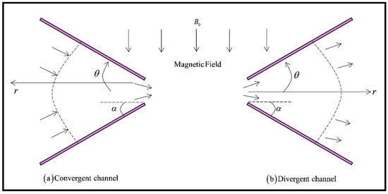
Figure 1.
Jeffery-Hamel flow in a converging/diverging channel with angle (Adapted from Motsa, et al. [12]).
After using Equation (6), Equations (1)–(5) reduce to the form
with boundary conditions
Now Equations (7)–(9) are converted into non-dimensional form after using the following dimensionless variables [7],
where is the wall temperature, is the dimensionless velocity parameter which can be obtained by dividing to its maximum value is the dimensionless temperature. Substituting Equation (10) into Equations (7)–(9) and after simplification, we have finally
subject to boundary conditions
where and be the Reynolds number and square of the Hartmann number respectively. Also, the Eckert number Ec and Prandtl numbers are defined as [32]
3. Solution by Using Spectral Homotopy Analysis Method
In the next section, the nonlinear boundary value problem describes in Equations (11)–(14) will be solved by using the spectral homotopy analysis method [12]. In order to apply the spectral homotopy analysis method to the problem, we suppose the initial guess satisfying the boundary conditions Equations (13) and (14) for the above problem is
The problem domain is first transformed from to using the following mapping from to x as
To convert non-homogeneous boundary conditions into homogeneous form, define the following transformations
After substituting Equation (17), in Equations (11)–(14) the boundary value problem reduces to the form
subject to boundary conditions
where primes denote the derivatives with respect to x and
For initial approximation, solution of the non-homogeneous linear part of the governing Equation (18) is obtained by using the Chebyshev pseudospectral method, that is
subject to boundary conditions
Here is approximated as a truncated series of Chebyshev polynomial as
where is the Chebyshev polynomial, are coefficients and are Gauss-Lobatto collocation points [5] defined as
and s order derivative of at this collocation points are
Here is the Chebyshev spectral differentiation matrix [5]. Substituting Equations (25)–(27) into Equations (23) and (24), given
subject to boundary conditions
and
Here
where T represents the transpose and diag is a diagonal matrix of order Now, we utilise the boundary conditions (29), by deleting the first and last rows and columns of matrix and deleting the first and last rows of and On the resulting last row of modified matrix , the boundary condition (30) is imposed and replacing the resulting last row of the modified matrix by zero. Hence it can be calculated by
which is considered as an initial approximation for the solution of Equation (18), using the spectral homotopy analysis method. Now, define a linear operator as
where q is the embedding parameter, which is defined by the homotopy analysis method and is an unknown function. So, the zeroth-order deformation equation is given by Makukula et al. [33]
where is convergence controlling parameter and is a nonlinear operator defined as
The order deformation equations are
subject to the boundary conditions
where
By applying the Chebyshev pseudospectral transformation [5] on Equations (36)–(38), we have
and
subject to the boundary conditions
and
where
Now for boundary conditions (41), the first and last rows of and , and the first and last rows and first and last columns of A in (39) are deleted. Also, to incorporate the boundary condition (42), the first row of and the first row and column are deleted. Boundary condition (44) is imposed on the last row of the modified matrix , and the last row of the modified matrix is replaced by zero. Therefore, the recursive formulas for is given by,
Hence by using the initial approximation, obtained by Equation (32), we can find the higher-order approximation and for using recursive formula (Equation (49)) and (Equation (50)). Thus, once is obtained, we can calculate from Equation (50). The techniques used in this section are based on the techniques of spectral homotopy analysis method as described in Motsa et al. [12] and Motsa et al. [34].
4. Results and Discussion
This variation of temperature profile with viscous dissipation under the effects of various parameters like; Eckert number , Reynold number , angle and Prandtl number are analyzed. The spectral homotopy analysis method is used to obtain the results for temperature profile with different values of parameters as shown graphically in Figure 2, Figure 3, Figure 4, Figure 5, Figure 6, Figure 7, Figure 8, Figure 9, Figure 10 and Figure 11. Figure 2, Figure 3, Figure 4, Figure 5 and Figure 6 shows the effects of parameters on temperature profile by considering diverging channel flow. As shown in Figure 2, which maps the effects of Reynold number on temperature profile, it is evident that temperature increases with the increase in Reynold number. There is a smooth increase in the temperature profile with varying Prandtl number and Eckert number , as in Figure 3 and Figure 4. Figure 5 shows that temperature profile increases when the angle of wall increases. Now, the case is quite the opposite for Hartmann number in the diverging channel, that is, with the increase in Hartmann number , temperature profile decreases. This is clear from Figure 6. Figure 7, Figure 8, Figure 9, Figure 10 and Figure 11 show the effects of this parameter on temperature profile when converging channel flow is under consideration. It is worth noting in Figure 7, with the increase in Reynold number , temperature profile decreases but does not show similar behaviour to the case of diverging channel flow. However, Figure 8, shows the behaviour of Prandtl number on temperature profile is very similar to the case of diverging channel flow. Temperature profile also increases in the case of increasing Eckert number shown in Figure 9, as in the case of the diverging channel flow profile. In the case of converging channel flow temperature profile is quite opposite to that of the converging channel with the increasing magnitude of wall angle depicted in Figure 10. Also, Figure 11 shows the effects of the Hartmann number on the temperature profile. With the increment of the Hartmann number, there is a slight decrease in the temperature profile. Table 1 and Table 2 show the effects of magnetic field on skin friction and Nusselt number taken for different values of Hartmann number H. Numerical values obtained by SHAM are also calculated using an approximate analytical technique known as the differential transform method (DTM) and a traditional numerical technique, known as the shooting method.
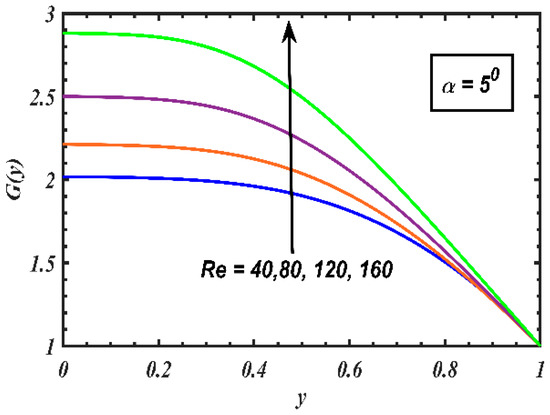
Figure 2.
Variation of G(y) in diverging channel for Re = 40, 80, 120, 160 and .
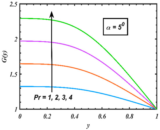
Figure 3.
Variation of G(y) in diverging channel for Pr = 1, 2, 3, 4 and .
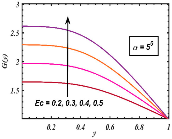
Figure 4.
Variation of G(y) in diverging for Ec = 0.2, 0.3, 0.4, 0.5 and .
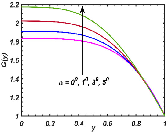
Figure 5.
Variation of G(y) in diverging channel for and .
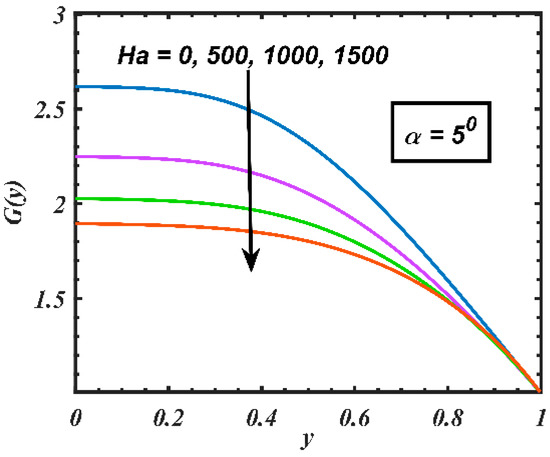
Figure 6.
Variation of G(y) in diverging channel for H = 0, 500, 1000, 1500 and .
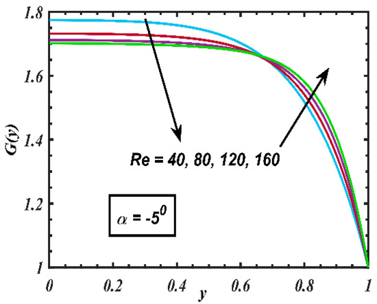
Figure 7.
Variation of G(y) in converging channel for Re = 40, 80, 120, 160 and .
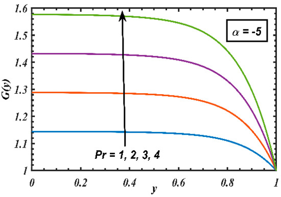
Figure 8.
Variation of G(y) in converging channel for Pr = 1, 2, 3, 4 and H = 0, Re = 100, α = −50, Ec = 0.5.
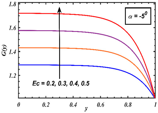
Figure 9.
Variation of G(y) in converging for Ec = 0.2, 0.3, 0.4, 0.5 and .
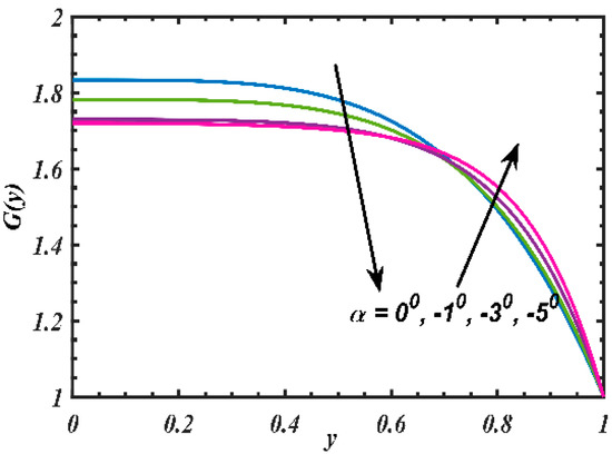
Figure 10.
Variation of G(y) in converging channel for α = 00, −10, −30, −50 and .
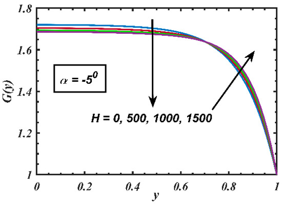
Figure 11.
Variation of G(y) in converging channel for H = 0, 500, 1000, 1500 and .

Table 1.
Comparison of the differential transform method (DTM) and shooting results with the spectral homotopy analysis method (SHAM) approximate results for when for increasing values of H.
Table 2.
Comparison of the DTM and shooting results with the SHAM approximate results for. when for increasing values of .
The comparison of SHAM results up to third-order SHAM with both of the techniques showed excellent agreement up to six decimal places.
5. Conclusions
In this study, heat transfer effects were analyzed in MHD converging/diverging channel flows. These effects are shown graphically in Figure 2, Figure 3, Figure 4, Figure 5, Figure 6, Figure 7, Figure 8, Figure 9, Figure 10 and Figure 11 and numerically in Table 1 and Table 2. A newly developed spectral homotopy analysis method (SHAM) by Motsa et al. [12] was used to calculate the results. The numerical values for skin friction and Nusselt number for varying Hartmann number are depicted in Table 1 and Table 2. They were also calculated using the DTM and the shooting method. SHAM third-order results matched with the DTM and the shooting method, showing that SHAM is feasible as a technique to be used.
6. Future Work
The present study has ignored the effect of nanofluid and porous medium, which are also relevant to various chemical dynamical systems. Future studies will aim to examine hybrid nanofluid over a thermoelastic porous medium [31,35,36].
Author Contributions
Conceptualization, A.M. and M.F.M.B.; Methodology, A.M.; Software, U.A.; Validation, M.A.M.; Formal analysis, A.M.; Investigation, M.F.M.B.; Writing—Original draft preparation, M.F.M.B.; Writing—Review and editing, U.A.; Visualization, A.M. and M.S.M.K.; Supervision, M.S.M.K.; Project administration, M.A.M.; Funding acquisition, M.A.M.
Funding
This research was funded by USM, grant number 304/PJJAUH/8312450 and the APC was funded by USM.
Conflicts of Interest
The authors declare no conflict of interest.
References
- Sibanda, P.; Motsa, S.; Makukula, Z. A spectral-homotopy analysis method for heat transfer flow of a third-grade fluid between parallel plates. Int. J. Numer. Methods Heat 2012, 22, 4–23. [Google Scholar] [CrossRef]
- Poff, N.L.; Allan, J.D.; Bain, M.B.; Karr, J.R.; Prestegaard, K.L.; Richter, B.D.; Sparks, R.E.; Stromberg, J.C. The natural flow regime. BioScience 1997, 47, 769–784. [Google Scholar] [CrossRef]
- Ahmed, N.; Abbasi, A.; Khan, U.; Mohyud-Din, S.T. Thermal radiation effects on flow of Jeffery fluid in converging and diverging stretchable channels. Neural Comput. Appl. 2018, 30, 2371–2379. [Google Scholar] [CrossRef]
- Banks, W.; Drazin, P.; Zaturska, M. On perturbations of Jeffery-Hamel flow. J. Fluid Mech. 1988, 186, 559–581. [Google Scholar] [CrossRef]
- Domairry, D.G.; Mohsenzadeh, A.; Famouri, M. The application of homotopy analysis method to solve nonlinear differential equation governing Jeffery–Hamel flow. Commun Nonlinear Sci. 2009, 14, 85–95. [Google Scholar] [CrossRef]
- Esmaili, Q.; Ramiar, A.; Alizadeh, E.; Ganji, D. An approximation of the analytical solution of the Jeffery–Hamel flow by decomposition method. Phys Lett. A 2008, 372, 3434–3439. [Google Scholar] [CrossRef]
- Ganji, Z.; Ganji, D.D.; Esmaeilpour, M. Study on nonlinear Jeffery–Hamel flow by He’s semi-analytical methods and comparison with numerical results. Comput. Math. Appl. 2009, 58, 2107–2116. [Google Scholar] [CrossRef]
- Patel, N.; Meher, R. Analytical investigation of Jeffery-Hemal flow with magnetic field by differential transform method. Int. J. Adv. Appl. Math. Mech. 2018, 6, 1–9. [Google Scholar]
- Dey, P.K.; Zikanov, O. Turbulence and transport of passive scalar in magnetohydrodynamic channel flows with different orientations of magnetic field. Int. J. Heat Fluid Flow 2012, 36, 101–117. [Google Scholar] [CrossRef]
- Guchhait, S.K.; Jana, R. A Study of Some Magnetohydrodynamics Problems with or Without Hall Currents; Vidyasagar University: West Bengal, India, 2018. [Google Scholar]
- Hvasta, M.; Dudt, D.; Fisher, A.; Kolemen, E. Calibrationless rotating Lorentz-force flowmeters for low flow rate applications. Meas. Sci. Technol. 2018, 29, 075303. [Google Scholar] [CrossRef]
- Motsa, S.S.; Sibanda, P.; Awad, F.G.; Shateyi, S. A new spectral-homotopy analysis method for the MHD Jeffery–Hamel problem. Comput. Fluids 2010, 39, 1219–1225. [Google Scholar] [CrossRef]
- Balazadeh, N.; Sheikholeslami, M.; Ganji, D.D.; Li, Z. Semi analytical analysis for transient Eyring-Powell squeezing flow in a stretching channel due to magnetic field using DTM. J. Mol. Liq. 2018, 260, 30–36. [Google Scholar] [CrossRef]
- Usman, M.; Hamid, M.; Khan, U.; Din, S.T.M.; Iqbal, M.A.; Wang, W. Differential transform method for unsteady nanofluid flow and heat transfer. Alex. Eng. J. 2018, 57, 1867–1875. [Google Scholar] [CrossRef]
- Ali, J. Application of New Iterative Method and Adomian Decomposition Method to Hamel’s Flow Problem. J. Adv. Civ. Eng. 2018, 4, 10–13. [Google Scholar] [CrossRef]
- Bakodah, H.O.; Ebaid, A. The adomian decomposition method for the slip flow and heat transfer of nanofluids over a stretching/shrinking sheet. Rom. Rep. Phys. 2018, 70, 115. [Google Scholar]
- Sobamowo, M.G.; Yinusa, A.A. Transient Combustion Analysis for Iron Micro-particles in a Gaseous Oxidizing Medium Using Adomian Decomposition Method. J. Comput. Eng. Phys. Model. 2018, 1, 1–15. [Google Scholar] [CrossRef]
- Ahmad, I.; Ilyas, H. Homotopy Perturbation Method for the nonlinear MHD Jeffery–Hamel blood flows problem. Appl. Numer. Math. 2019, 141, 124–132. [Google Scholar] [CrossRef]
- Shirkhani, M.; Hoshyar, H.; Rahimipetroudi, I.; Akhavan, H.; Ganji, D. Unsteady time-dependent incompressible Newtonian fluid flow between two parallel plates by homotopy analysis method (HAM), homotopy perturbation method (HPM) and collocation method (CM). Propul. Power Res. 2018, 7, 247–256. [Google Scholar] [CrossRef]
- Ahmad, H. Variational iteration method with an auxiliary parameter for solving differential equations of the fifth order. Nonlinear Sci. Lett. A 2018, 9, 27–35. [Google Scholar]
- Dogan, D.D.; Konuralp, A. Fractional variational iteration method for time-fractional non-linear functional partial differential equation having proportional delays. Therm. Sci. 2018, 14, 33–46. [Google Scholar] [CrossRef]
- Inc, M.; Khan, H.; Baleanu, D.; Khan, A. Modified variational iteration method for straight fins with temperature dependent thermal conductivity. Therm. Sci. 2018, 8, 229–236. [Google Scholar] [CrossRef]
- Wazwaz, A.-M.; Kaur, L. Optical solitons and Peregrine solitons for nonlinear Schrödinger equation by variational iteration method. Optik 2019, 179, 804–809. [Google Scholar] [CrossRef]
- Fei, J.; Lin, B.; Yan, S.; Zhang, X. Approximate solution of a piecewise linear–nonlinear oscillator using the homotopy analysis method. J. Vib. Control 2018, 24, 4551–4562. [Google Scholar] [CrossRef]
- Liu, J.; Wang, B. Solving the backward heat conduction problem by homotopy analysis method. Appl. Numer. Math. 2018, 128, 84–97. [Google Scholar] [CrossRef]
- Noeiaghdam, S.; Araghi, M.A.F.; Abbasbandy, S. Finding optimal convergence control parameter in the homotopy analysis method to solve integral equations based on the stochastic arithmetic. Numer. Algorithms 2018, 1, 237–267. [Google Scholar] [CrossRef]
- Rana, P.; Shukla, N.; Gupta, Y.; Pop, I. Homotopy analysis method for predicting multiple solutions in the channel flow with stability analysis. Commun. Nonlinear Sci. Numer. Simul. 2019, 66, 183–193. [Google Scholar] [CrossRef]
- Bhatti, M.M.; Abbas, M.A.; Rashidi, M.M. A robust numerical method for solving stagnation point flow over a permeable shrinking sheet under the influence of MHD. Appl. Math. Comput. 2018, 316, 381–389. [Google Scholar] [CrossRef]
- Shahid, A.; Zhou, Z.; Bhatti, M.; Tripathi, D. Magnetohydrodynamics Nanofluid Flow Containing Gyrotactic Microorganisms Propagating Over a Stretching Surface by Successive Taylor Series Linearization Method. Microgravity Sci. Technol. 2018, 30, 445–455. [Google Scholar] [CrossRef]
- Shivanian, E.; Alsulami, H.; Alhuthali, M.; Abbasbandy, S. Predictor homotopy analysis method (PHAM) for nano boundary layer flows with nonlinear Navier boundary condition: Existence of four solutions. Filomat 2014, 28, 1687–1697. [Google Scholar] [CrossRef]
- Othman, M.I.; Marin, M. Effect of thermal loading due to laser pulse on thermoelastic porous medium under GN theory. Results Phys. 2017, 7, 3863–3872. [Google Scholar] [CrossRef]
- Moradi, A.; Alsaedi, A.; Hayat, T. Investigation of heat transfer and viscous dissipation effects on the Jeffery-Hamel flow of nanofluids. Therm. Sci. 2015, 19, 563–578. [Google Scholar] [CrossRef]
- Makukula, Z.G.; Sibanda, P.; Motsa, S.S. A Novel Numerical Technique for Two-Dimensional Laminar Flow between Two Moving Porous Walls. Math. Probl. Eng. 2010, 2010, 528956. [Google Scholar] [CrossRef]
- Motsa, S.S.; Shateyi, S.; Marewo, G.T.; Sibanda, P. An improved spectral homotopy analysis method for MHD flow in a semi-porous channel. Numer. Algorithms 2012, 60, 463–481. [Google Scholar] [CrossRef]
- Marin, M. Contributions on uniqueness in thermoelastodynamics on bodies with voids. Cienc. Mat. (Havana) 1998, 16, 101–109. [Google Scholar]
- Hassan, M.; Marin, M.; Ellahi, R.; Alamri, S.Z. Exploration of convective heat transfer and flow characteristics synthesis by Cu–Ag/water hybrid-nanofluids. Heat Transf. Res. 2018, 49, 1837–1848. [Google Scholar] [CrossRef]


© 2019 by the authors. Licensee MDPI, Basel, Switzerland. This article is an open access article distributed under the terms and conditions of the Creative Commons Attribution (CC BY) license (http://creativecommons.org/licenses/by/4.0/).