In this section, we first derive the explicit control law of the unconstrained MPC, which includes two parts: (i) the future target information feedforward, and (ii) the output feedback. Based on the future target information feedforward, we demonstrate that a poor future trajectory horizon has quite an impact on the system’s performance. Then we propose an optimization method to determine the future trajectory horizon and the tripe-mode model predictive control using future target information. The triple-mode MPC is composed of the designed unconstrained control law and the extra degrees of freedom. The future target information is taken into account explicitly to improve tracking performance.
3.1. Illustrations of Poor Future Trajectory Horizon
Now we show that the unconstrained MPC control law will provide possibilities in the explicit expression of feedforward and feedback. Consider the performance objective
in problem (5), one can derive the unconstrained law by minimizing it w.r.t the future control moves, according the extremum condition
, we have
and making the following substitutions
then we can get
It can be seen that the future target information is involved in the first term of the control law: , which can be seen as the feedforward in the unconstrained control law. In addition, the second part of the control law can be seen as the output feedback based on the current output prediction.
For convenience, we define the future trajectory horizon in feedforward term for each output as
, which indicates the length of future target information considered in the optimization. Any future targets beyond the future trajectory horizon will not be taken into account in the optimization problem, even if known. For a given
, the future target information adopted in MPC can be expressed as
Furthermore, by combining the specific future trajectory horizon, the unconstrained law can be represented as follows:
where
refers to the
ith feedforward contribution, and
is the reconstructed future target information feedforward component based on the designed future trajectory horizon
.
and
denotes the
jth column vector of the feedforward matrix
.
It indicates that, for the ith output, the original P-dimension target vector has been replaced by a designed -dimension vector . A major current focus in improving the control performance is how to select a proper . It is known that the typical DMC algorithm considers no setpoint changes during the optimizaiton, which is equivalent to set the future trajectory horizon as .
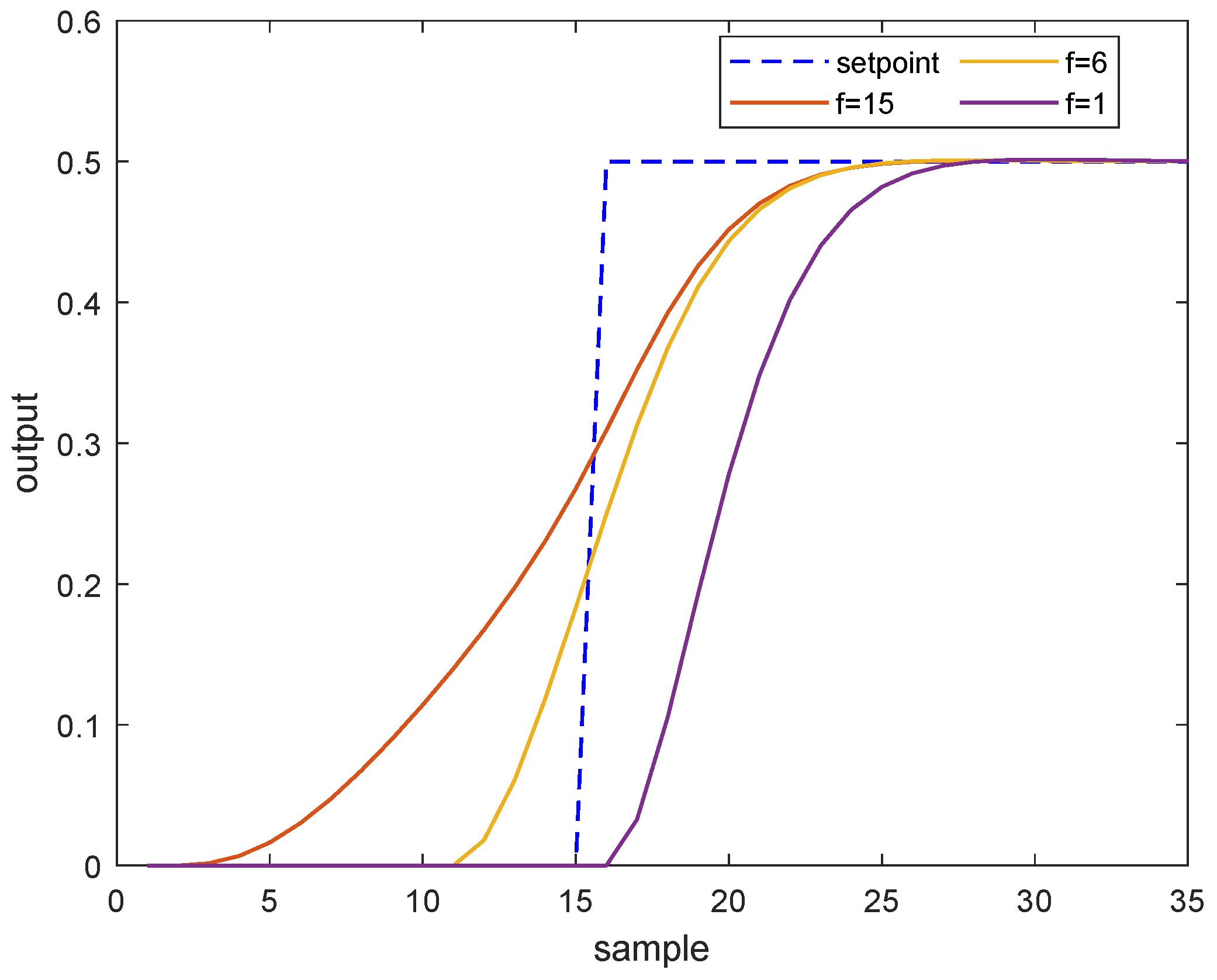
Next, we examine the closed-loop performances of the MPC algorithm adopting different choices of future trajectory horizon. Consider a single-input, single-output system described by the following transfer function
The sampling time is chosen as 5 s, a step change of setpoint happens at sampling instant 15 and the unconstrained MPC algorithm is applied to drive the system to its target. The arbitrary choices of future trajectory horizon are . The tuning parameters of DMC are: and in which I is the identity matrix.
As illustrated by
Figure 1, with a default choice of future trajectory horizon in MPC (
), the system response is slugglish when the setpoint changes, in contrast, setting the future trajectory horizon as the prediction horizon could result in an aggressive response. A proper selection
deserves a desirable tracking performance.
The integral of squared error (ISE) criterion is widely used to evaluate the system performance in control engineering, the discrete form of ISE reads
in which
refers to the difference between the expected value (target value) and the actual response value at time instant
t.
The ISE values shown in
Table 1 demonstrate that the standard MPC algorithm with no anticipation (
) owns large ISE value during the transition from one target to another. On the other hand, with large number of future trajectory horizon (
), the system would react far in advance and lead to bad performance too.
3.3. Triple-Mode MPC Algorithm Using Future Target Information
For the conventional MPC algorithm, the optimization problem (5) is solved with degree of freedom to tackle constraints. However, the original optimization problem treats the input as decision variables, which breaks down the inherent future target information feedforward structure as described before. What’s more, the default choice of future trajectory horizon in the MPC algorithm may lead to sluggish tracking performance. There exists no effective method to determine a proper future target horizon for MPC optimization.
With the proposed Algorithm 1 used, we next present a triple-mode MPC algorithm using future target information. Different from the typical DMC algorithm as described in preliminary section, the proposed triple-mode control law encompasses three parts: (i) the future target information feedforward, (ii) the output feedback, and (iii) the extra degrees of freedom. Each mode of the control law can be designed individually. The first two parts of the control law are off-line designed through unconstrained MPC, and the optimal future trajectory horizon is obtained by using Algorithm 1. The final part is calculated by the on-line MPC algorithm aiming to satisfy constraints.
Enhance the unconstrained MPC control law Equation (
8) with an additional term
in which
and
representing degrees of freedom to get the constraints satisfied.
It indicates that the original degree of freedom
in constrained DMC optimization (5) is replaced by
, which not only provide the feedforward design from future target information but also guarantee the advantage of constraint satisfaction. At each sampling time, the controller solves the following optimization problem
where Equation (17f) refers to the terminal constraint used to ensure closed-loop stability when model predictive control is employed. After optimization, the optimal solution
can be obtained, and the optimal input increment is nothing but
with
. Note that the proposed triple-mode MPC optimiazation problem (17) is a quadratic programming [
18] with
degrees of freedom. The degrees of freedom are the same as the original DMC optimization problem (5), thus the computation load of proposed triple-mode MPC is the same as which of DMC.
A detailed implementation procedure of the proposed triple-mode MPC algorithm (Algorithm 2) is summarized as follows.
| Algorithm 2: Triple-mode MPC algorithm using future target information |
Offline computation: Carry out the Algorithm 1 to obtain the future trajectory horizon , the first two parts of the control law are designed through Equations ( 7) and ( 10); Online computation: Step 1. At sampling time t, controller receives measurement from the sensors and evaluate the modified estimate of predictions according to Equation ( 4); Step 2. Solve the optimization problem (17) to evaluate its future input trajectory; Step 3. Injects the optimal input into the plant; Step 4. Set , and go to Step 1.
|
In this section, the triple-mode MPC using future target information is presented. As has been previously stated, this triple-mode control law is based on the usage of the perturbations on the fixed dual-mode unconstrained control law. To this end, the following assumption is considered.
Assumption A1. The step response sequenceis a Cauchy sequence:.
Assumption A2. The weighting matricesandare positive definite matrices. At least as many inputs as outputs is required:.
The future target is admissible if there exist a set of control sequence such that the system output can reach it and the constraints (e.g., ) can be satisfied during the stage. The following theorem follows immediately.
Theorem 1. Consider that Assumption 1 and 2 hold, and the future target is admissible. Then, for any feasible initial state , the proposed triple-mode controller asymptotically steers the system to .


