Abstract
The paper concerns the modeling of heterogeneous biofilm growth on fine spherical particles of such biofilm forms as, e.g., fluidized-bed bioreactors. Three discrete mathematical models based on cellular automata theory were proposed. The double-substrate kinetics of biomass growth, biomass displacement, internal and external mass transfer resistances, death and lysis of microbiological cells and biofilm detachment were taken into account. It was shown that there are no significant qualitative and quantitative differences between biofilm growth on flat and spherical particles of different radii. Computer simulations were compared with experimental observations. Qualitative and quantitative agreement areachieved if both cell death and lysis aretaken into consideration and a proper algorithm of biomass displacement is used. The value of the bacteria lysis rate coefficient was estimated.
1. Introduction
The biological processes of wastewater treatment can be divided into suspended-, attached- and mixed-growth ones. In suspended-growth processes, microorganisms flow freely in the liquid phase. Microorganisms in attached-growth processes grow on solid substratum in theform of a biofilm, whereas, in mixed-growth processes, both forms are present in a system. Particle-based biofilm reactors, in which fine particles are used as a substratum for biofilm growth, have been widely employed in numerous processes, including the biodegradation of pollutants [1] and the production of antibiotics [2]. Reactors belonging to this group; for example, fluidized-bed bioreactors and air-lift suspension bioreactors can be operated at high volumetric flow rates, since the biomass is immobilized on a solid carrier of highly developed interphase surface, and retained inside the reactor [3].
Numerous studies have been published during last five decades concerning modeling and understanding the processes occurring in biofilms. The first mathematical models of biofilms assumed aflat geometry and a uniform distribution of biomass [4]. Those models were used for describing the utilization and diffusion of a single limiting substrate. Advances in experimental techniques, such as microelectrode technology and confocal scanning laser microscopy (CSLM), enabled researchers to determine the structure of biofilm more accurately and to verify the results of computer simulations [5]. Discoveries concerning heterogeneous biofilm growth induced an interest in the modeling of biofilm structure. The effect of studies in this area are two- and three-dimensional mathematical models based on a properly defined grid (cellular automata) [6,7,8] andon individuals (individual-based models) [9].
Several cellular automata-based models of the biofilm growth have been published so far. However, no model is able to predict the morphology and structure of biofilm growing on fine spherical particles. One of the few studies in this area is the work by Graf von Schulenburg et al. [10], who proposed a discrete model of biofilm growth in porous media. However, the quoted authors accepted the single-substrate Monod kinetic model and neglected biofilm detachment.
In this study, three models based on cellular automata are proposed. The first one neglects death and the lysis of microbiological cells and a previously published algorithm of biomass displacement is used. The second one takes into account the death of microorganisms, while the third one allows for the death and lysis of microorganisms. Moreover, a new algorithm of biomass displacement is proposed. Dynamical simulations of biofilm growth were performed using the proposed models and compared. The relationships between average biofilm density and its thickness were compared with those obtained experimentally.
2. Mathematical Model of the Biofilm Dynamics
The mathematical model is based on the two-dimensional cellularautomata model of biofilm growth on flat substratum presented in a previous study [11,12]. It was modified in order to represent growth on spherical particles. The model takes into account the diffusion and utilization of two growth-limiting substrates, the spreading of biomass and biofilm detachment. The nextmodification was introduced in order to take into account death and the lysis of bacterial cells.
The cellular automata-based models differ in their approach tosimulating biomass spreading and cell death and lysis. Appendix A presents rules which were used in all models, namely“diffusion of the substrates”, “utilization of the substrates in the biofilm”, “growth of microorganisms and biofilm detachment”.
The formulated cellular automata differ in terms of the algorithm of biomass spreading used in the following ways:
- The algorithm of biomass spreading proposed by Picioreanu et al. [7]. Cell death and lysis are neglected. It will be further referred to as CA-1.
- The algorithm of biomass spreading proposed in this study. Cell death is taken into account. It will be further referred to as CA-2.
- An algorithm of biomass spreading that is the same as in CA-2. However, both death and lysis of microbiological cells are taken into account. It will be further referred to as CA-3.
The CA-1 model consists of three grids describing the concentration of biomass, carbonaceous substrate and oxygen. Due to the negligence of microbiological cell death, all biomass is active. Cellular automata CA-2 and CA-3 consist of four grids describing, respectively, concentrations of active biomass, dead (inert) biomass, carbonaceous substrate and oxygen. The cell states of each grid of the cellular automata correspond to ρba, ρbo, and , respectively.
In order to explain the algorithm for the death of microorganisms, let us consider the following kinetic expression of the biomass death rate:
At every time step Δtg, the biomass density will decrease due to the death of bacteria:
where i and j are indices of the grid.
The death of active bacteria is connected with the generation of dead (inactive) microbiological cells. Therefore, the cell state of the grid representing the concentration of dead bacteria will change according to:
Experimental studies indicate that inert biomass loses its mechanical properties [13]. The process of bacterial lysis is modeled in this study as a first-order process. Only dead cells are subject to this phenomenon:
A similar approach was used in the cellular automata-based model proposed by Pizarro et al. [14]; however, this model used single-substrate kinetics and flat biofilm.
Algorithm for Biomass Spreading Used in CA-2 and CA-3
According to Tang and Valochi [15] the application of the algorithm proposed by Picioreanu et al. [7] results in significant discontinuities in the biomass distribution. Instead of a probabilistic algorithm for the biomass spreading, Tang and Valochi proposed a deterministic one, based on the determination of theshortest path from the source grid cell to the destination cell. Based on the observations of the quoted authors, the following algorithm was formulated.
- Checkif the following condition is fulfilled:If yes, go to step 2. Otherwise, finish the algorithm.
- Calculate the amount of biomass thatexceeds the maximum density:
- Calculate the amount of active and dead bacteria in the value calculated in point 1, as follows:
- Determine the concentrations of active and dead bacteria in time t + Δt:
- Find a grid cell with indices [i2, j2] at the lowest distance from [i, j] for which the following condition is fulfilled:
- Change the concentrations inthe target cells:
3. Dynamics of the Biofilm Growth
The computer program implementing the CA-1 model generates results in the form of three two-dimensional arrays at each time moment. Each array represents concentrations of biomass and two liming substrates: carbonaceous substrate A and oxygen T. For mathematical models thattake into account dead cells, i.e., CA-2 and CA-3, an additional array is created to represent dead bacteria. The value of each cell in a grid, i.e., the cell state, indicates the concentration of a given component.
The aerobic degradation of phenol was chosen as a process example due to the large significance of this process in wastewater treatment. Moreover, several experimental studies can be found in the literature, which can be used for the validation of model predictions [16,17,18]. The kinetic parameters of this process are presented in Table 1.

Table 1.
Kinetic parameters of aerobic degradation of phenol by Pseudomonas putida [19].
Figure 1 shows two-dimensional distributions of biomass (Figure 1a–d), phenol (Figure 1e–h) and oxygen (Figure 1i–l) concentrations at different growth times t for biofilm grown on a particle with a radius equal to 150 μm. The chosen value corresponds to sand particles commonly used in fluidized-bed bioreactors. The results presented in Figure 1 were obtained with the use of CA-1, i.e., with the negligence of cell death and lysis. It was accepted that, at an initial time, the particle is uniformly covered with biomass of density equal to . The concentrations of phenol and oxygen in the bulk liquid were equal to 0.02 kg/m3 and 0.008 kg/m3, respectively. The chosen dissolved oxygen concentration is close to the saturation state.
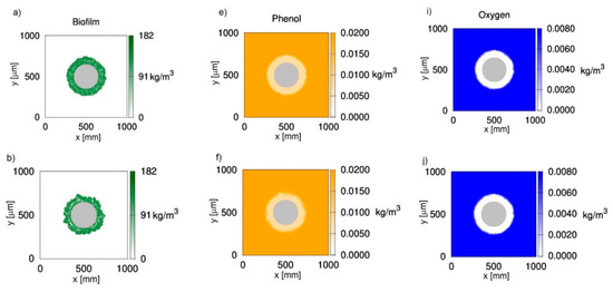
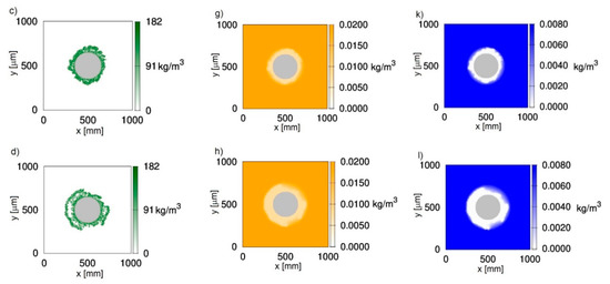
Figure 1.
Evolution of the biofilm growth on a particle of radius rz = 150 μm; left column—biomass density; middle column—phenol concentration; right column—oxygen concentration; successive rows represent time moments: (a,e,i) t = 50 h; (b,f,j) t = 100 h; (c,g,k) t = 150 h; (d,h,l) t = 200 h; values on vertical and horizontal axes are expressed in μm.
It can be seen in Figure 1 that oxygen was depleted in deeper parts of the biofilm (Figure 1i–l), while phenol penetrated the whole biofilm (Figure 1e–h). Such behavior is related to the large requirement foroxygen in this process, which is reflected by yield coefficients wBA and wBT. According to these values, the utilization of 1 kg of phenol is related to the utilization of 1.54 kg of oxygen. Even if the biofilm thickness is relatively low, approximately 100 μm (Figure 1c), the biofilm is not fully penetrated by oxygen.
The biomass distributions presented in Figure 1 show that biofilm thickness may decrease during the process. Thisis due to sloughing, i.e., a phenomenon based on the sudden detachment of large portions of the biofilm. It occurs when external parts of the biofilm lose their connection with deeper layers attached to the substratum. The sloughing event is illustrated more clearly in Figure 2, where the relationship between maximum biofilm thickness and time is shown. This mechanism occurs twice during 200 h of the process. At a growth time equal to 86 h, the biofilm thickness decreased from approximately 121 μm to 87 μm, while, at 145 h, sloughing occurred for the second time.
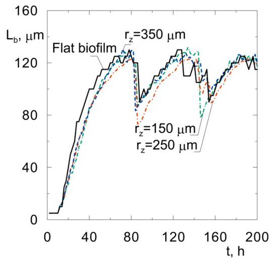
Figure 2.
Biofilm thickness vs. time of biofilm growth on spherical particles of different radiiand on a flat substratum.
The occurrence of sloughing is related to the existence of voids in the middle of the biofilm (Figure 1b–d). This property is caused by the mutual influence of the biofilm detachment (shear) and oxygen depletion. According to the accepted detachment model [20], the probability of this phenomenon is proportional to the square of the distance from the carrier surface. The biomass, which is placed near the biofilm surface, is more susceptible to the detachment;however, the substrates are available in larger amounts, which facilitates biomass growth. In turn, the growth of biomass near the carrier substratum is limited due to the depletion of oxygen, but the detachment probability is low due to the small distance from the carrier surface.
The radii of sand particles used in fluidized-bed bioreactors vary in the range of about 100–400 μm [3]. Other materials can also be used as a substratum for biofilm growth. For example, Seker et al. [21] used carbon particles with a radius equal to 250 μm. It is justified to perform an analysis of the influence of the size of an inert particle on the biofilm structure. Computer simulations were performed for spherical particles with radiibetween 150 μm and 350 μm and for a flat substrata, for comparison. The relationships between the biofilm thickness and time for all simulated biofilms arepresented in Figure 2. Close qualitative and quantitative agreement can be seen. In every case, the sloughing occurs after about 80 h at abiofilm thickness of approximately 125 μm. The phenomenon occurs for the second time when the biofilm thickness reaches approximately 125 μm once again. Such fluctuations inthe biofilm thickness have been observed in laboratory experiments, for example, in the study by Horn et al. [22]. The phenomenon was called a “quasi-steady state” by the quoted authors.
Figure 3 presents two-dimensional distributions of active and inert biomass obtained with the use of CA-2 for time moments equal to t = 50 h (Figure 3a,e, i.e., first row), t = 100 h (Figure 3b,f, i.e., second row), t = 150 h (Figure 3c,g, i.e., third row) and t = 200 h (Figure 3d,h, i.e., fourth row). The value of thecell death rate coefficient was accepted according to Kumar et al. [23], i.e., ko = 5.6 × 10⁻³ 1/h. It can be seen in Figure 3a,e that at t = 50 h, despite relatively large biofilm thickness, almost all bacteria are active, i.e., their concentrations are close to . The dead bacteria concentrations are significantly lower. Thisis caused by the large difference between the biomass growth rate and death rate, i.e.,the value of k is approximately 100 times larger than ko. The biofilm growth rate is relatively large; therefore, 50 h of growth is sufficient for obtaining athickness over 80 μm. Due to the significantly lower death rate coefficient, inactive bacteria did not accumulate due to the short growth time. Inactive bacteria accumulates near the substratum, i.e., at the biofilm bottom. This is related to the utilization of substrates during transfer into the biofilm. Bacteria located at the carrier surface are subject to the lowest substrate concentrations; therefore, the growth is limited in this region. The distributions of inactive bacteria after larger values of time (Figure 3f–h) show that concentrations of inactive bacteria continuously increase at the biofilm bottom. Aggregation in this region is also related to a low detachment probability near the carrier surface. In turn, dead bacteria near the biofilm external surface are continuously removed due to the detachment. The depletion of substrates in deeper biofilm partsalso results in lower active biomass concentrations.
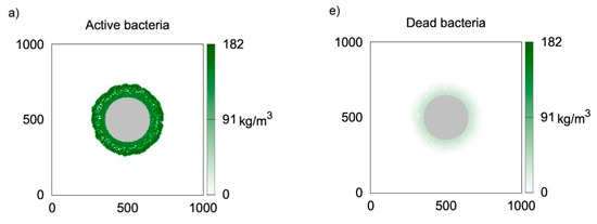
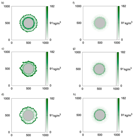
Figure 3.
Two-dimensional distributions of active (left) and inert (right) biomass density in spherical biofilm obtained with the use of CA-2; values on vertical and horizontal axes are expressed in μm; successive rows represent time moments: (a,e) t = 50 h; (b,f) t = 100 h; (c,g) t = 150 h; (d,h) t = 200 h.
Similar simulations were performed using the CA-3 model, i.e., bytaking into account the death and lysis of microbiological cells. Due to a lack of experimental data concerning this phenomenon, the value of klys = 1.12 h−1 was used, i.e., twice larger than the death rate coefficient. Simulations later in the study were performed for different values of this coefficient. Two-dimensional distributions of active and inert biomass are presented in Figure 4 in a similar manner as in Figure 3. At the initial stage of biofilm formation, bothdistributions of active biomass (Figure 4a,e) are very similar to thosepresented in Figure 3a,e, respectively. However, for longer growth times, significantly lower inert biomass concentrations are obtained when lysis is taken into consideration. Thiscan be seen in Figure 3f–h. Surprisingly, thisdoes not affect low active biomass concentrations at the biofilm bottom. Thiscan be explained by the depletion of oxygen, and therefore the lack of biomass growth in this biofilm region.
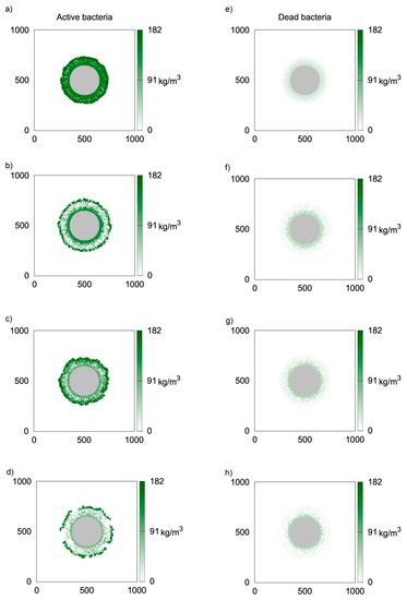
Figure 4.
Two-dimensional distributions of active (left) and inert (right) biomass density in spherical biofilm obtained with the use of CA-3 (klys = 1.12 h−1); values on vertical and horizontal axes are expressed in μm; successive rows represent time moments: (a,e) t = 50 h; (b,f) t = 100 h; (c,g) t = 150 h; (d,h) t = 200 h.
4. Comparison of Model Predictions with Experimental Observations
The results of several experiments of phenol degradation by Pseudomonas putida conducted in fluidized-bed bioreactors can be found in the literature. According to the results of these studies, the relationship is a straight line, andis presented in Figure 5. Thusfar, no model has been published which predicts such biomass distribution. It should be noted that the results of the quoted experiments were conducted in different process conditions, whichexplains the different slopes of the obtained lines. The density distribution in the biofilm depends on, among other things, the type of fluidized bed (i.e., two-phase or three-phase), the number of particles in the bed and the species of bacteria [24]. The presence of bubbles in the bed results in higher detachment rates. This phenomenon is also intensified by larger particle numbers due to an increased frequency of collisions.
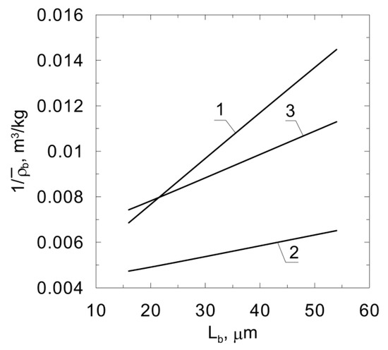
Figure 5.
Relationships obtained based on experimental studies; line‘1’ [16,17]; line‘2’ [18]; line‘3’ [25].
The goal of this part of the study was to choose the model where the predictions of which fit the experimental data most accurately. Dynamic simulations were performed for seven values of the bulk liquid carbonaceous substrate concentration between and . After a sufficiently long time, i.e., when a quasi-steady state was reached, average biomass concentration and thickness werecalculated. The relationship was obtained using cellular automata CA-1, CA-2 and CA-3 for different values of lysis rate coefficient. Based on the obtained results, the linearity of relationships was evaluated by determining the coefficients of determination, R2. The calculated values are summarized in Table 2. It can be seen that both the cell death rate coefficient and cell lysis rate coefficient influence the linearity of the relationship . The highest value of R2 was obtained for klys = 1.12 × 10⁻² 1/h. The obtained function is presented in Figure 6. It canalso be seen in Table 2 that the biomass spreading algorithm proposed by Picioreanu et al. [7] is characterized by the lowest R2 value. According to the authors of this study, the mentioned biomass spreading algorithm should not be used for the modeling of biofilm growth. The results obtained confirm the conclusions drawn by Tang and Valocchi [15] that the probabilistic biomass spreading algorithm results in unrealistic biomass distributions.
Table 2.
Coefficients of determination for straight lines fitted to relationships obtained using cellular automata-based models.
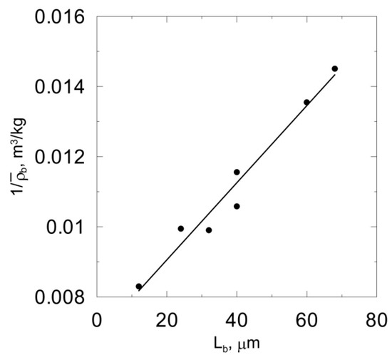
Figure 6.
Relationships obtained using CA-3 model and klys =1.12 × 10⁻² 1/h.
5. Conclusions
Three cellular automata-based models of biofilm growth are proposed in thisstudy. The first one neglects the death and lysis of microbiological cells, and uses a previously published algorithm of biomass displacement. The second one takes into account the death of microorganisms, while the third one allows for the death and lysis of microorganisms. A new algorithm of biomass displacement is also proposed.
The obtained results prove that both the death and lysis of microorganisms significantly influence the biofilm structure. The models were validated by a comparison of the relationships between average biomass density and biofilm thickness, obtained numerically, with those obtained experimentally by Seker et al. [19]. The results of phenol degradation by Pseudomonas putida in fluidized-bed bioreactors were used for this purpose. It was shown that, in order to obtain relationships corresponding to the experimental ones, it is necessary to use a proper approach to biomass displacement and to take into account the death and lysis of microorganisms. Moreover, the value of the lysis rate coefficient was estimated.
Author Contributions
Conceptualization, preparation of computer programs, realization of simulations, S.S.; interpretation of results, draft preparation, S.S. and M.C.-S. All authors have read and agreed to the published version of the manuscript.
Funding
This research received no external funding.
Conflicts of Interest
The authors declare no conflict of interest.
Nomenclature
| cA, cB, cT | mass concentration of carbonaceous substrate, biomass and oxygen (kg∙m−3) |
| De | effective diffusion coefficient in biofilm (m2∙h−1) |
| k | maximum specific growth rate (h−1) |
| Kdet | detachment probability coefficient |
| ko | cell death rate coefficient (h−1) |
| klys | cell lysis rate coefficient (h−1) |
| Lb | total thickness of the biofilm (m) |
| rA, rT | uptake rate of carbonaceous substrate and oxygen, respectively (kg∙m−3∙h−1) |
| pdet | detachment probability |
| rB | growth rate of biomass (kg∙m−3∙h−1) |
| rz | radius of the inert particle (μm) |
| t | time (h) |
| wBA, wBT | growth yield coefficients (kg B∙(kg A)−1), (kg B∙(kg T)−1) |
| x | distance from the carrier surface (m) |
| Δt | time step for diffusion and utilization processes (h) |
| Δtg | time step for biomass growth and detachment (h) |
| ρb | concentration of biomass in the biofilm (kg∙m−3) |
| ρbo | concentration of dead bacteria in the biofilm (kg∙m−3) |
| ρba | concentration of active biomass in biofilm phase (kg∙m−3) |
| maximum biomass concentration in the biofilm (kg∙m−3) | |
| Superscripts | |
| b | biofilm phase |
| c | liquid (continuous) phase |
| Subscripts | |
| A, B, T | refers to carbonaceous substrate, biomass and oxygen, respectively |
| a | active bacteria |
| b | biofilm |
| o | dead bacteria |
Appendix A. Rules Governing the Cellular Automata
Rule 1—Diffusion of the Substrates
The probabilities of the movement of the mass quantum of oxygen in the liquid phase in all four directions on the grid are the same and equal to PdTw, and the sum of these probabilities is equal to one. The probability of the movement of the mass quantum of oxygen is dependent on the presence of biomass in the starting and the target cell. It was calculated as follows [12]:
The above equation is useful for both the water and the biofilm. In Equation (A1), nb is the number characterizing the system of two cells: the starting and the target one. Thisspecifies the sum of the cells in this doublet, which represent the biomass. In turn, nw is the number related to the presence of water in the same doublet of cells. Both nb and nw can take values from the set {0,1,2}.
Similarly, as was done above for the oxygen transfer process, the relationship defining the probability PdA of the displacement of the mass quantum of the carbonaceous substrate is as follows:
It was assumed that the ratio of the probability of the mass quantum displacement of the carbonaceous substrate in water to the probability of the mass quantum displacement of oxygen in the water is equal to the ratio of diffusion coefficients in water, PdAw/PdTw = DAw/DTw.
Rule 2—Utilization of the Substrates in the Biofilm
The rates of utilization of the carbonaceous substrate rA and oxygen rT in the biofilm are described by Equations (A3) and (A4)
The forms of functions f1 and f2 depend on a given microbiological process. For the aerobic degradation of phenol, they take the form of Equations (A5) and (A6), respectively:
Using the equation defining the reaction rate related to substrate A, we have
Based on the above relationship, the expressions determining the increases in the concentrations of substrates during the time step ∆t can be obtained. These expressions are shown below:
The new values of the cells’ states in the grids for the substrates are
Rule 3—Growth of Microorganisms and Biofilm Detachment
Due to the significantly different values of the characteristic times of diffusion and utilization and those of the growth of biomass and biofilm detachment [9], this rule is performed for larger time step valuesin theorder of hours [11].
The increase in the mass of active microorganisms in one time step Δtg is determined using Equation (A12)
The new value of the cell’s state is then
To calculate the probability of the biofilm detachment, Equation (A14) was used, as proposed by Chambless et al. [20].
where x is the distance from the carrier surface.
References
- Tanyolaç, A.; Beyenal, H. Prediction of average biofilm density and performance of a spherical bioparticle under substrate inhibition. Biotechnol. Bioeng. 1997, 56, 319–329. [Google Scholar] [CrossRef]
- Al-Qodah, Z. Antibiotics production in a fluidized bed reactor utilizing a transverse magnetic field. Bioprocess Eng. 2000, 22, 299–308. [Google Scholar] [CrossRef]
- Nicolella, C.; van Loosdrecht, M.C.M.; Heijnen, S.J. Particle-based biofilm reactor technology. Trends Biotechnol. 2000, 18, 312–320. [Google Scholar] [CrossRef]
- Atkinson, B.; Daoud, I.S.; Williams, D.A. A theory for biological film reactor. Trans. Inst. Chem. Eng. Chem. Eng. 1968, 46, 245–250. [Google Scholar]
- Julian, W.; Werner, M.; Ulrich, S. Heterogeneity in biofilms. FEMS Microbiol. Rev. 2006, 24, 661–671. [Google Scholar]
- Picioreanu, C.; van Loosdrecht, M.C.M.; Heijnen, J.J. Mathematical modeling of biofilm structure with a hybrid differential-discrete cellular automaton approach. Biotechnol. Bioeng. 1998, 58, 101–116. [Google Scholar] [CrossRef]
- Picioreanu, C.; van Loosdrecht, M.C.M.; Heijnen, J.J. A new combined differential-discrete cellular automaton approach for biofilm modeling: Application for growth in gel beads. Biotechnol. Bioeng. 1998, 57, 718–731. [Google Scholar] [CrossRef]
- Xavier, J.B.; Picioreanu, C.; Van Loosdrecht, M.C.M. A modelling study of the activity and structure of biofilms in biological reactors. Biofilms 2004, 1, 377–391. [Google Scholar] [CrossRef][Green Version]
- Wanner, O.; Eberl, H.J.; Morgenroth, E.; Noguera, D.R.; Picioreanu, C.; Rittmann, B.E.; van Loosdrecht, M.C.M. Mathematical Modeling of Biofilms; WA Scientific and Technical Report No. 18; IWA Task Group on Biofilm Modeling: London, UK, 2006. [Google Scholar]
- Graf von der Schulenburg, D.A.; Pintelon, T.R.R.; Picioreanu, C.; van Loosdrecht, M.C.M.; Johns, M.J. Three-dimensional simulations of biofilm growth in porous media. AIChE J. 2008, 55, 494–504. [Google Scholar] [CrossRef]
- Skoneczny, S. Cellular automata-based modelling and simulation of biofilm structure on multi-core computers. Water Sci. Technol. 2015, 72, 2071–2081. [Google Scholar] [CrossRef]
- Skoneczny, S. Cellular automata as an effective tool for modelling of biofilm morphology. Environ. Prot. Eng. 2017, 43, 177–190. [Google Scholar] [CrossRef]
- Bishop, P.L.; Zhang, T.C.; Fu, Y.-C. Effects of biofilm structure, microbial distributions and mass transport on biodegradation processes. Water Sci. Technol. 1995, 31, 143–152. [Google Scholar] [CrossRef]
- Pizarro, G.E.; Garcia, C.; Moreno, R.; Sepulveda, M.E. Two-dimensional cellular automaton model for mixed-culture biofilm. Water Sci. Technol. 2004, 49, 193–198. [Google Scholar] [CrossRef]
- Tang, Y.; Valocchi, A.J. An improved cellular automaton method to model multispecies biofilms. Water Res. 2013, 47, 5729–5742. [Google Scholar] [CrossRef] [PubMed]
- Karel, S.F.; Libicki, S.B.; Robertson, C.R. The immobilization of whole cells: Engineering principles. Chem. Eng. Sci. 1985, 40, 1321–1354. [Google Scholar] [CrossRef]
- Tang, W.-T.; Wisecarver, K.; Fan, L.-S. Dynamics of a draft tube gas-liquid-solid fluidized bed bioreactor for phenol degradation. Chem. Eng. Sci. 1987, 42, 2123–2134. [Google Scholar] [CrossRef]
- Beyenal, H.; Tanyolaç, A. The effects of biofilm characteristics on the external mass transfer coefficient in a differential fluidized bed biofilm reactor. Biochem. Eng. J. 1998, 1, 53–61. [Google Scholar] [CrossRef]
- Seker, S.; Beyenal, H.; Salih, B.; Tanyolac, A. Multi-substrate growth kinetics of Pseudomonas putida for phenol removal. Appl. Microbiol. Biotechnol. 1997, 47, 610–614. [Google Scholar]
- Chambless, J.D.; Stewart, P.S. A three-dimensional computer model analysis of three hypothetical biofilm detachment mechanisms. Biotechnol. Bioeng. 2007, 97, 1573–1584. [Google Scholar] [CrossRef]
- Şeker, Ş.; Beyenal, H.; Tanyolaç, A. The effects of biofilm thickness on biofilm density and substrate consumption rate in a differential fluidizied bed biofilm reactor (DFBBR). J. Biotechnol. 1995, 41, 39–47. [Google Scholar] [CrossRef]
- Horn, H.; Reiff, H.; Morgenroth, E. Simulation of growth and detachment in biofilm systems under defined hydrodynamic conditions. Biotechnol. Bioeng. 2003, 81, 607–617. [Google Scholar] [CrossRef] [PubMed]
- Kumar, A.; Kumar, S.; Kumar, S. Biodegradation kinetics of phenol and catechol using Pseudomonas putida MTCC 1194. Biochem. Eng. J. 2005, 22, 151–159. [Google Scholar] [CrossRef]
- Tabiś, B.; Siudzińska, R. Ocena rozkładów gęstości i współczynników dyfuzji w biofilmie immobilizowanym na materiale drobnoziarnistym. Przem. Chem. 2005, 84, 250–253. [Google Scholar]
- Beyenal, H.; Şeker, Ş.; Tanyolaç, A.; Salih, B. Diffusion coefficients of phenol and oxygen in a biofilm of Pseudomonas putida. AIChE J. 1997, 43, 243–250. [Google Scholar] [CrossRef]


© 2020 by the authors. Licensee MDPI, Basel, Switzerland. This article is an open access article distributed under the terms and conditions of the Creative Commons Attribution (CC BY) license (http://creativecommons.org/licenses/by/4.0/).