Mathematical Model of COVID-19 Transmission Dynamics in South Korea: The Impacts of Travel Restrictions, Social Distancing, and Early Detection

Abstract

The novel coronavirus disease (COVID-19) poses a severe threat to public health officials all around the world. The early COVID-19 outbreak in South Korea displayed significant spatial heterogeneity. The number of confirmed cases increased rapidly in the Daegu and Gyeongbuk (epicenter), whereas the spread was much slower in the rest of Korea. A two-patch mathematical model with a mobility matrix is developed to capture this significant spatial heterogeneity of COVID-19 outbreaks from 18 February to 24 March 2020. The mobility matrix is taken from the movement data provided by the Korea Transport Institute (KOTI). Some of the essential patch-specific parameters are estimated through cumulative confirmed cases, including the transmission rates and the basic reproduction numbers (local and global). Our simulations show that travel restrictions between the epicenter and the rest of Korea effectively prevented massive outbreaks in the rest of Korea. Furthermore, we explore the effectiveness of several additional strategies for the mitigation and suppression of Covid-19 spread in Korea, such as implementing social distancing and early diagnostic interventions.

1. Introduction

The first case of the novel coronavirus, severe acute respiratory syndrome coronavirus 2 (SARS-CoV-2), was reported by Chinese health officials in Wuhan City in December 2019. Coronaviruses are a family of viruses that can cause illnesses, such as severe acute respiratory syndrome and the Middle East respiratory syndrome [1]. The clinical spectrum of COVID-19 infection is broad, ranging from no symptoms to severe pneumonia. Approximately half of the COVID-19 patients (40–50%) in one study did not show any symptoms [2]. Other patients developed fever, body aches, nausea, or diarrhea [3] typically 2 to 14 days after exposure to the virus. During the initial phase of COVID-19 in China (10–23 January 2020), only $14\%$ of total infections were confirmed. The remaining 86% were not identified or quarantined, contributing to a community spread in China. Later, on 23 January, the Chinese government implemented a total lockdown of Wuhan City, which prevented further community spread [4]. Owing to this strict intervention, the number of new COVID-19 cases in China dropped to the single-digits in early March. Other countries, however, started to report an increasing number of confirmed cases. COVID-19 spread from Wuhan to the rest of China and neighboring Asian countries such as Thailand, Japan, Korea, Singapore, and Hong Kong. As of 31 March, the number of confirmed cases worldwide had exceeded 820,000, and the number of deaths had reached more than 40,000 in more than 110 countries. The World Health Organization declared COVID-19 a pandemic on 11 March 2020 ([5,6]).

In South Korea, the first confirmed case of COVID-19 was reported on 20 January, and the number of cases steadily increased to 30 by 17 February. Beyond the initial sporadic outbreaks from overseas inflows, including China, there was a large-scale community spread around specific regions. Beginning with the 31st confirmed case on 18 February, however, an unprecedented rapid increase of confirmed cases was recorded in the area of Daegu and North Gyeongsang Province (Gyeongbuk). It is still unclear how or from whom the 31st case became infected. Daegu is Korea’s 4th largest city and is surrounded by Gyeongbuk (see Figure 1). In the process of tracing the contacts of the 31st case on 18 February, it was revealed that she attended worship services at the Sincheonji Daegu Church on 9 February and 16 February, raising the possibility of community spread through the church service. Indeed, an inspection of more than 1000 Sincheonji Daegu members on 20 February resulted in the identification of more than 111 cases. Epidemiological surveillance of these 111 newly identified cases revealed that most cases presented to Cheongdo Daenam Hospital in Gyeongbuk. Health authorities later imposed cohort isolation on the hospital after a large cluster of COVID-19 cases was reported. Although most of the confirmed cases were concentrated in Daegu or Gyeongbuk, COVID-19 spread to nearly every part of the country [7]. Across the nation, 79.7% of the cases have been proven to be linked to cluster transmission, and 62.5% have been linked to Shincheonji [8]. As of 31 March 2020, 9786 patients were confirmed in Korea, 7984 of whom (81%) were confirmed in Daegu and Gyeongbuk [8]. The spread of COVID-19 in Korea displayed a spatial heterogeneity, a clustered rapid spread in Daegu and Gyeongbuk, and a steady slow spread in the rest of the country.

Mathematical modeling can provide useful insights for mitigating emerging infectious diseases such as recent SARS-CoV, MERS-CoV, COVID-19 outbreaks. Particularly, the mathematical modeling of the spread of diseases becomes more important as the movement of people and other living organisms increases due to globalization [9,10]. Multi-patch models have been developed to understand the global spread of transmission dynamics in various emerging and reemerging infectious diseases [11,12,13,14]. Since the COVID-19 outbreak began, many studies have been carried out to investigate the basic or control reproductive numbers, whereas others predicted the outbreak peak time and evolution of the epidemic to guide intervention policies ([15,16,17,18]). The national and global spread of COVID-19 was explored, accounting for the effect of the metropolitan-wide quarantine of Wuhan and surrounding cities [19]. A stochastic transmission model was combined with COVID-19 data from Wuhan City to estimate the temporal evolution of transmission [20]. The study also predicted the probability of how newly introduced cases would generate outbreaks in other areas. Time-varying basic reproduction number has been investigated in Italy and forecasted the COVID-19 spread in the region [21]. The critical role of a latency period is highlighted under three different modeling of latency periods in SEIR-based models [22]. Some studies investigated the effectiveness of COVID-19 mitigation strategies, such as travel restrictions ([23,24]) and social distancing ([25,26,27,28]). These nonpharmaceutical measures reduced transmissibility by a maximum of $34\%$ without resorting to a strict lockdown strategy [29].

In this study, we develop a two-patch model of COVID-19 transmission dynamics, representing a hot spot (patch 1: Daegu and Gyeongbuk) and a slow-spreading area (patch 2: the rest of Korea). In each patch, we employed a mathematical model with five epidemiological compartments (susceptible, exposed, infected, quarantined, and recovered), which is based on the previous work [14]. The two patches are connected by a mobility matrix that captures the number of people traveling in South Korea (provided by the Korea Transport Institute (KOTI) in 2016) [30]. It includes origin and destination data on various modes of transportation, including airplanes, cars, buses, ships, and trains. The incubation and recovery rates were assumed to be the same in the two areas and other parameters such as transmission rate were assumed to be different in the two patches and were estimated using cumulative incidence data from 18 February to 24 March 2020. Using the estimated model parameters, we carried out a patch-specific sensitivity analysis. Furthermore, we investigated the impacts of various intervention strategies on the patch-specific transmission dynamics, including limiting traveling between the two regions, implementing social distancing, and early diagnosis.

This paper is organized as follows. In Section 2, we present a data description followed by a single-patch SEIQR model and a two-patch SEIQR model with a mobility matrix and discuss the basic reproduction numbers (the local reproduction number for a single-patch model and the global reproduction number for a two-patch model). We have carried out parameter estimation and sensitivity analysis in Section 3. Numerical simulations under various mitigation scenarios have been investigated in Section 4. The paper concludes with a discussion of results and conclusions in Section 5 and Section 6. Following Section 6, we include the Appendix A containing the mathematical work, showing the derivation of the basic reproduction number for a two-patch SEIQR model.

2. Data and Model

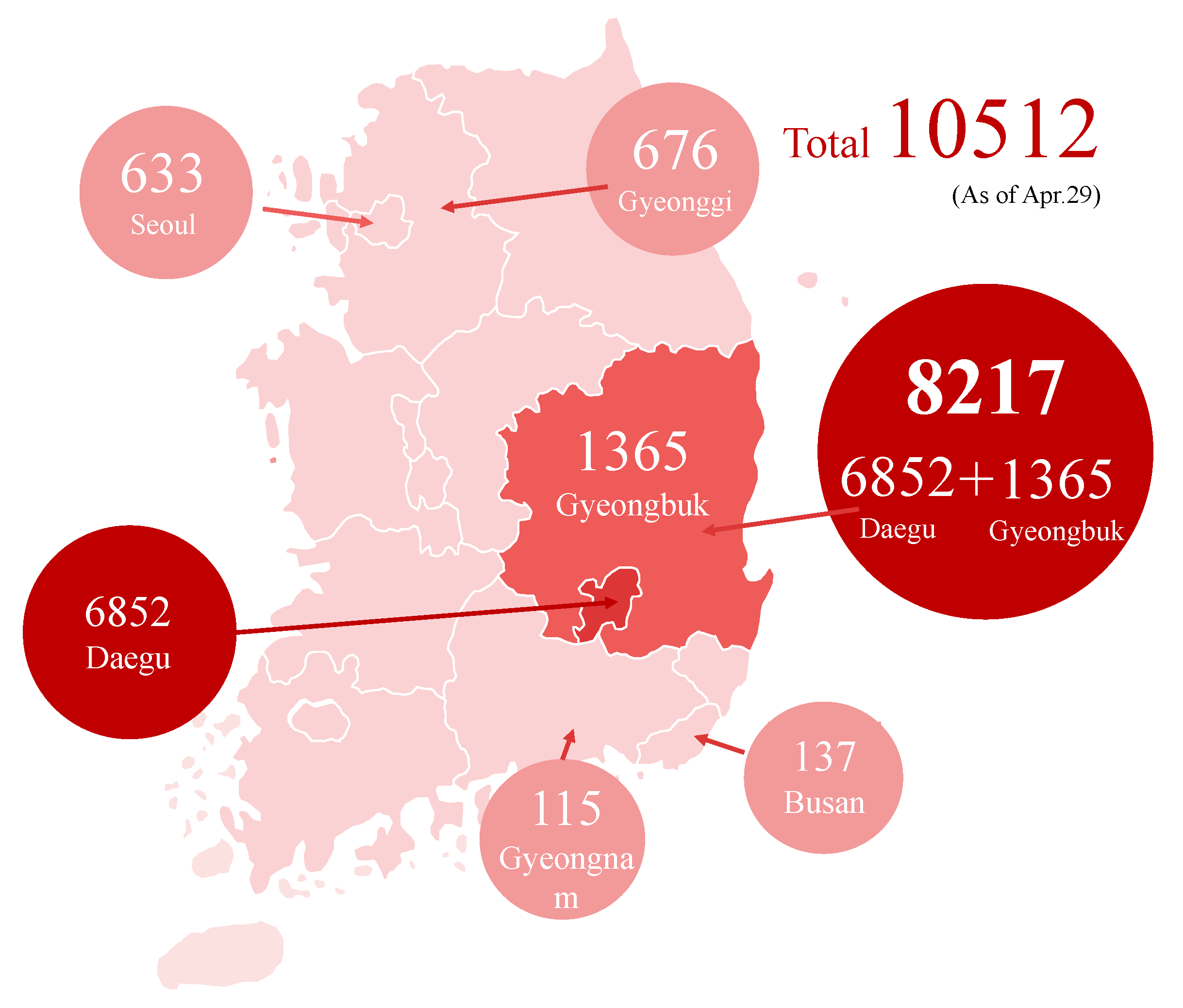
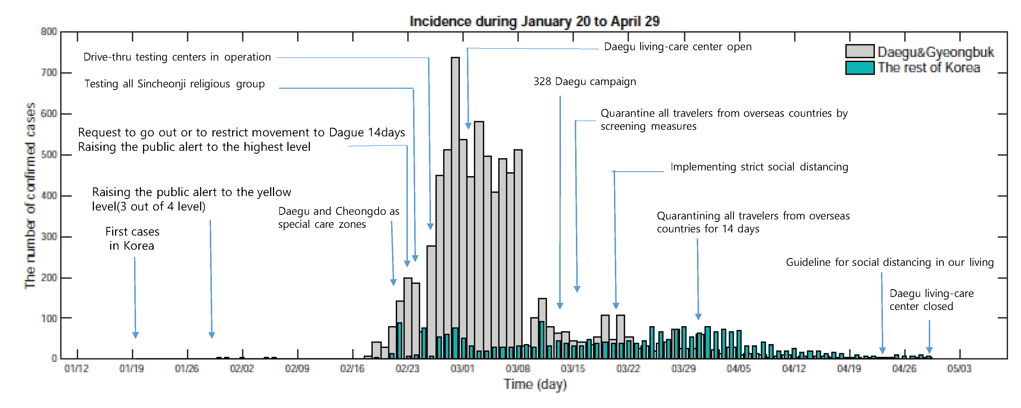
2.1. Characteristics of the Early COVID-19 Outbreaks in South Korea

Daily confirmed cases in South Korea were publicly available from the Korea Centers for Disease Control and Prevention (KCDC) [31,32]. Due to the 31st case, a rapid increase occurred, especially in the Daegu/Gyeongbuk area, and Figure 2 displays the daily confirmed cases in Daegu/Gyeongbuk and the rest of Korea. The spatial characteristics of cumulative incidence are displayed in Figure 1. Note that there were hot spots in Daegu and Gyeongbuk, which were around 80% of the total cases, implying a high level of spatial heterogeneity in the number of confirmed cases of Korea.

The timeline of administrative measures in Daegu and Gyeongbuk is displayed in Figure 2 and

Table 1. Administrative countermeasures implemented by the Korean government (Daegu and Gyeongbuk) [31,32].

Date	Administrative Countermeasures
20 January	The first case reported in Korea
28 January	Raising the public alert to the yellow level (3 out of 4 level)
3 February	Self-quarantine followed by contact-tracing
21 February	Declare Daegu and Cheongdo as special care zones
23 February	Restrict movement in Dague 2 weeks
	Raising the public alert to the highest level
24 February	Testing all Sincheonji religious group, - Delay schools open
26 February	Supply of face masks export restriction and sale for public purpose
	Drive-through testing centers in operation
2 March	Daegu living-care center open
5 March	Gyeongbuk as a special management zone
15 March	328 Daegu campaign (minimization of movement, and social distancing)
17 March	Quarantine all travelers from overseas countries
21 March	Strict social distancing
22 March	COVID-19 testing at all nursing hospitals in Daegu almost completed
1 April	Quarantining all travelers from overseas countries for 14 days
4 April	Strict social distance extended
9 April	Schools begin online classes
20 April	Mitigated social distancing
22 April	Prepare sustainable social distancing
24 April	Guideline for social distancing in our living
30 April	Daegu living-care center closed

. The Korean government and Dague and Gyeongbuk implemented administrative countermeasures in response to COVID-19 outbreaks (as shown in Table 1) [31,32]. On 17 February, the first drive-through testing facility was installed, where symptom checks and sample collection could be performed in less than 10 min. The Korean government declared Daegu and Gyeongbuk as “special care zones” on 21 February. The Korean government upgraded the infectious disease crisis alert to the severe level on 23 February and requested citizens of Daegu to refrain from voluntarily going out and restricting their movement for at least 2 weeks. All schools were closed, and employees at many companies were working at home [7]. Prompt detection followed by isolation was advised to mitigate the spread of the infectious disease. Moreover, many medical professionals and administrative officials from the private sector volunteered to serve in Daegu. The citizens of Daegu begin to implement the “328 Dague movement”, including the minimization of movement, as well as social distancing.

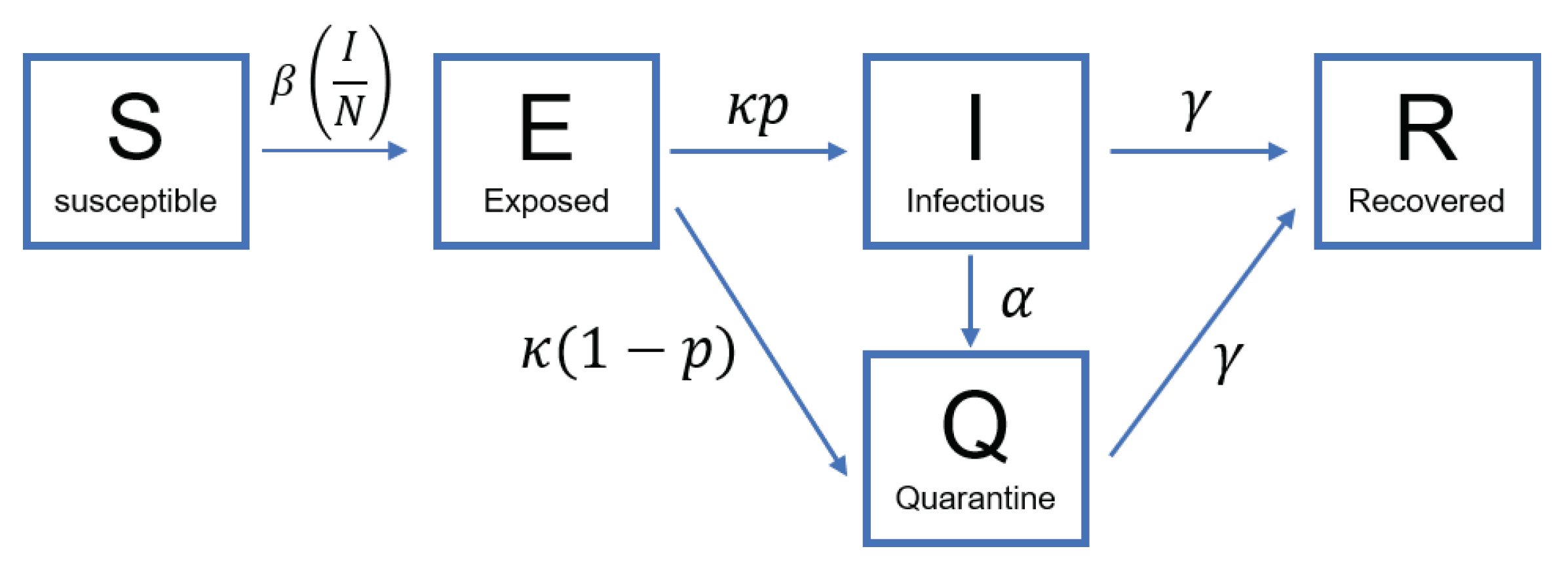
2.2. A Single-Patch Model: SEIQR Model

We first considered a single-patch SEIQR model. The birth and natural death of the population were not considered. The population was divided into five groups according to disease state. First, at time t, $S\left(t\right)$ is the number of susceptible individuals and $E\left(t\right)$ is the number of exposed individuals. Next, $I\left(t\right)$ denotes the number of infectious individuals, including asymptotic infection but not undetected (or not confirmed) individuals. Finally, $Q\left(t\right)$ represents the number of confirmed and therefore, quarantined individuals, while $R\left(t\right)$ represents the number of recovered individuals. From the schematic diagram depicted in Figure 3, we have the following system of five ordinary differential equations:

$$\left\{\begin{array}{c}\begin{array}{cc}\hfill \frac{dS}{dt}& =-\beta \left(\frac{I}{N}\right)S,\hfill \\ \hfill \frac{dE}{dt}& =\beta \left(\frac{I}{N}\right)S-\kappa E,\hfill \\ \hfill \frac{dI}{dt}& =\kappa pE-\alpha I-\gamma I,\hfill \\ \hfill \frac{dQ}{dt}& =\kappa (1-p)E+\alpha I-\gamma Q,\hfill \\ \hfill \frac{dR}{dt}& =\gamma Q+\gamma I,\hfill \end{array}\hfill \end{array}\right.$$

(1)

where $N\left(t\right)=S\left(t\right)+E\left(t\right)+I\left(t\right)+Q\left(t\right)+R\left(t\right)$ at time t. Here, $\beta$ represents the transmission rate, and $\kappa$ is the rate of exposed people ($E\left(t\right)$) to become infectious ($I\left(t\right)$), p represents a proportion from $E\left(t\right)$ to $I\left(t\right)$ (asymptomatic and undetected but infectious individuals), $\alpha$ stands for the rate of quarantined, and $\gamma$ represents a recovery rate (either from $I\left(t\right)$ or $Q\left(t\right)$). The definitions and values of all model parameters are listed in

Table 2. Baseline parameter descriptions and values.

Parameter	Description	Value	Reference
$m_{12}$	The number of people traveling from patch 1 to patch 2 per day	2,192,794	[30]
$m_{21}$	The number of people traveling from patch 2 to patch 1 per day	1,693,727	[30]
${\kappa }_1$	Progression rate from E to I in patch 1 per day	1/7	[34]
${\kappa }_2$	Progression rate from E to I in patch 2 per day	1/7	[34]
${\gamma }_1$	Recovery rate in patch 1	1/14 per day	[35]
${\gamma }_2$	Recovery rate in patch 2	1/14 per day	[35]
$p_1$	The proportion of undetected infectious individuals in patch 1	0.33	[36]
$p_2$	The proportion of undetected infectious individuals in patch 2	0.33	[36]
$N_1\left(t\right)$	Population size in patch1 (Daegu and Gyeongbuk)	5.12 $\times {10}^6$	[37]
$N_2\left(t\right)$	Population size in patch2 (the rest of Korea)	46.52 $\times {10}^6$	[37]
$I_1\left(t_0\right)$	Initial number of asymptomatic individuals in patch1	1442	Estimated
$I_2\left(t_0\right)$	Initial number of asymptomatic individuals in patch2	330	Estimated
$t_1$	The starting point of the rapid increase interval	4	Estimated
$t_2$	The starting point of the slower increase interval	10	Estimated
${\beta }_{1,1}$	Transmission rate of patch 1 during $[t_0,t_1)$	0.338	Estimated
${\beta }_{1,2}$	Transmission rate of patch 1 during $[t_1,t_2)$	0.99	Estimated
${\beta }_{1,3}$	Transmission rate of patch 1 during $[t_2,t_{end})$	0.01	Estimated
${\beta }_2$	Transmission rate of patch 2 during $[t_0,t_{end})$	0.3575	Estimated
${\alpha }_1$	Early detection and diagnostic rate of patch 1 per day	0.0312	Estimated
${\alpha }_2$	Early detection and diagnostic rate of patch 2 per day	0.3575	Estimated

.

The dynamic behavior of the model can be classified by the basic reproductive number. This threshold condition determines whether an infectious disease will spread in a susceptible population when the disease is introduced into the population [33]. The threshold is calculated by using the next-generation method as

$${\mathcal{R}}_0=\rho \left(F{V}^{-1}\right),$$

where $\rho$ is defined as the spectral radius of the next-generation matrix $F{V}^{-1}$. Here, $\mathcal{F}$ is the rate of appearance of new infections, and $\mathcal{V}$ is the transfer of individuals out. Then, we find the Jacobian matrix of $\mathcal{F}\left(x\right)$ and $\mathcal{V}\left(x\right)$, and denote $F=[\partial {\mathcal{F}}_i/\partial x_j]$ and $V=[\partial {\mathcal{V}}_i/\partial x_j](i,j=1,2,\cdots ,5)$ evaluated at the disease free equilibrium point $E_{DFE}=(N,0,0,0,0)$. More details are given in the Appendix A. We can explicitly calculate the basic reproduction number, ${\mathcal{R}}_0$ (or the local reproduction number for a single-patch model) as

$${\mathcal{R}}_0=\frac{\beta p}{\alpha +\gamma }.$$

(2)

We concluded that $E_{DFE}$ is locally asymptotically stable if, and only if, ${\mathcal{R}}_0<1$. When ${\mathcal{R}}_0>1$, the matrix has a positive real eigenvalue, and this means that the disease-free equilibrium is unstable.

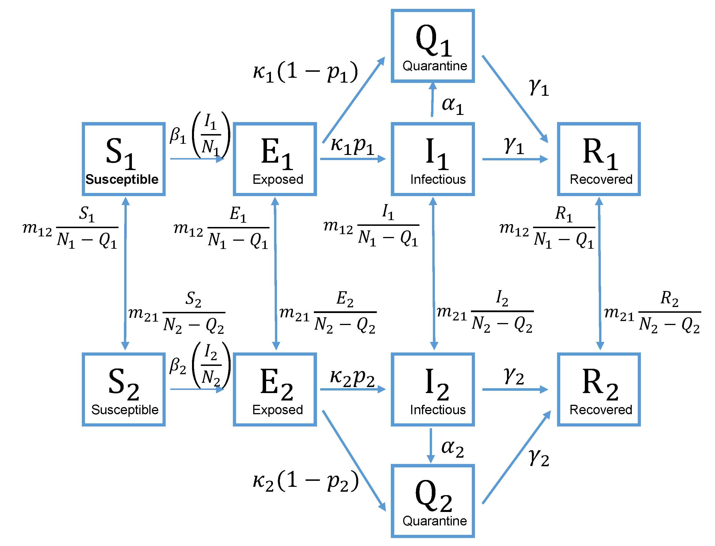
2.3. Two-Patch Transmission Model

In this subsection, we extended the single-patch model to the two-patch transmission model by incorporating the mobility matrix between the two patches. Other state variables and parameters are the same as the single-patch model given in the previous subsection. The mobility matrix is defined by $M={\left(m_{ij}\right)}_{2\times 2}$, as proposed in [13,14]. The mobility matrix captures the movement of individuals between patch 1 and patch 2 and we set $m_{ij}$ to be the number of people traveling from a patch i to a patch j per unit time (day) and $m_{ji}$ to be the number of people traveling from a patch j to a patch i per unit time (day). In this study, we assumed that the number of traveling between two patches is symmetric ($m_{ij}=m_{ji}$). Moreover, we assume that the quarantined individuals do not move to the other patch, the number of susceptible people entering patch i is $m_{ji}{S}_j/(N_j-Q_j)$, and the number of susceptible people leaving patch i is $m_{ij}{S}_i/(N_i-Q_i)$. It is also assumed that the traveling occurs instantaneously, so no infection is transmitted during the traveling process. As shown in the schematic diagram of the two-patch model, Figure 4, the following system of differential equations describes the resulting two-patch transmission model:

$$\left\{\begin{array}{c}\begin{array}{cc}\hfill \frac{d{S}_i}{dt}& =-{\beta }_i\left(\frac{I_i}{N_i}\right)S_i+m_{ji}\frac{S_j}{N_j-Q_j}-m_{ij}\frac{S_i}{N_i-Q_i},\hfill \\ \hfill \frac{d{E}_i}{dt}& ={\beta }_i\left(\frac{I_i}{N_i}\right)S_i-{\kappa }_i{E}_i+m_{ji}\frac{E_j}{N_j-Q_j}-m_{ij}\frac{E_i}{N_i-Q_i},\hfill \\ \hfill \frac{d{I}_i}{dt}& ={\kappa }_{i}p{E}_i-{\alpha }_i{I}_i-{\gamma }_i{I}_i+m_{ji}\frac{I_j}{N_j-Q_j}-m_{ij}\frac{I_i}{N_i-Q_i},\hfill \\ \hfill \frac{d{Q}_i}{dt}& ={\kappa }_i(1-p)E_i+{\alpha }_i{I}_i-{\gamma }_i{Q}_i,\hfill \\ \hfill \frac{d{R}_i}{dt}& ={\gamma }_i{I}_i+{\gamma }_i{Q}_i+m_{ji}\frac{R_j}{N_j-Q_j}-m_{ij}\frac{R_i}{N_i-Q_i},\hfill \end{array}\hfill \end{array}\right.$$

(3)

where $N_i=S_i+E_i+I_i+Q_i+R_i(i,j=1,2)$. It is assumed that p is the same in the both patches $p=p_1=p_2$) and that $\kappa$ (or $\gamma$) is the same in the both patches ($\kappa ={\kappa }_1={\kappa }_2$ and $\gamma ={\gamma }_1={\gamma }_2$). The descriptions and values of all model parameters are listed in Table 2.

For the two-patch model, the (global) basic reproduction number, ${\mathcal{R}}_0$, is computed by the next generation matrix approach [33] as

$${\mathcal{R}}_0=\rho \left(F{V}^{-1}\right),$$

where $\rho$ is defined as the spectral radius of the next-generation matrix $F{V}^{-1}$. Here, $\mathcal{F}$ is the rate of appearance of new infections, and $\mathcal{V}$ is the transfer of individuals out. Then, we find the Jacobian matrix of $\mathcal{F}\left(x\right)$ and $\mathcal{V}\left(x\right)$, and denote $F=[\partial {\mathcal{F}}_i/\partial x_j]$ and $V=[\partial {\mathcal{V}}_i/\partial x_j](i,j=1,2,\cdots ,4)$ evaluated at the disease free equilibrium point, $E_{DFE}=(N_1,0,0,0,0,N_2,0,0,0,0)$. Since the basic reproduction number is obtained by evaluating at the disease equilibrium under the assumption of the initial stage (i.e., $S_i\left(t\right)\equiv N_i\left(t\right)$), thus, we can replace $N_i\left(t\right)-Q_i\left(t\right)$ with $N_i\left(t\right)$ ($Q_i\left(t\right)\equiv 0$ at the the disease equilibrium point). The dynamics of infected compartments for a two-patch model can thus be described by

$$\begin{array}{cc}\hfill \frac{d{E}_1}{dt}& ={\beta }_1\left(\frac{I_1}{N_1}\right)S_1-\kappa E_1+{\overline{m}}_{21}{E}_2-{\overline{m}}_{12}{E}_1,\hfill \\ \hfill \frac{d{I}_1}{dt}& =\kappa p{E}_1-{\alpha }_1{I}_1-\gamma I_1+{\overline{m}}_{21}{I}_2-{\overline{m}}_{12}{I}_1,\hfill \\ \hfill \frac{d{E}_2}{dt}& ={\beta }_2\left(\frac{I_2}{N_2}\right)S_2-\kappa E_2+{\overline{m}}_{12}{E}_1-{\overline{m}}_{21}{E}_2,\hfill \\ \hfill \frac{d{I}_2}{dt}& =\kappa p{E}_2-{\alpha }_2{I}_2-\gamma I_2+{\overline{m}}_{12}{I}_1-{\overline{m}}_{21}{I}_2,\hfill \end{array}$$

(4)

where ${\overline{m}}_{12}=m_{12}/N_1$ and ${\overline{m}}_{21}=m_{21}/N_2.$

Indeed, we obtain the (global) basic reproduction number, ${\mathcal{R}}_0$ of the two-patch model as

$${\mathcal{R}}_0=\frac{\sqrt{C}+\kappa p{\beta }_1(D_3{D}_4+{\overline{m}}_{12}{\overline{m}}_{21})+{\beta }_2(D_1{D}_2+{\overline{m}}_{12}{\overline{m}}_{21})}{2({\overline{m}}_{12}{\overline{m}}_{21}-D_1{D}_3)({\overline{m}}_{12}{\overline{m}}_{21}-D_2{D}_4)},$$

(5)

where $D_1={\kappa }_1+{\overline{m}}_{12},D_2=\gamma +{\alpha }_1+{\overline{m}}_{12},D_3={\kappa }_2+{\overline{m}}_{21},D_4=\gamma +{\alpha }_2+{\overline{m}}_{21}$, and

$$\begin{array}{cc}\hfill C=& D_1^2{D}_2^2{\beta }_2^2{\kappa }_2^2{p}_2^2+D_3^2{D}_4^2{\beta }_1^2{\kappa }_1^2{p}_1^2+2(D_3{D}_4{\beta }_1^2+D_1{D}_2{\beta }_2^2){\kappa }_1{\kappa }_2{\overline{m}}_{12}{\overline{m}}_{21}{p}_1{p}_2+\hfill \\ \hfill & {\overline{m}}_{12}^2{\overline{m}}_{21}^2({\beta }_2^2{\kappa }_1^2{p}_1^2+{\beta }_1^2{\kappa }_2^2{p}_2^2)+\left(2{\beta }_1{\beta }_2{\overline{m}}_{12}{\overline{m}}_{21}\right)(D_1{D}_2{\kappa }_2^2{p}_2^2+D_3{D}_4{\kappa }_1^2{p}_1^2)+\hfill \\ & 4(D_1{D}_3+D_2{D}_4){\beta }_1{\beta }_2{\kappa }_1{\kappa }_2{\overline{m}}_{12}{\overline{m}}_{21}{p}_1{p}_2-(D_1{D}_2{D}_3{D}_4+{\overline{m}}_{12}^2{\overline{m}}_{21}^2)2{\beta }_1{\beta }_2{\kappa }_1{\kappa }_2{p}_1{p}_2.\hfill \end{array}$$

The details of the above derivations are given in Appendix A.

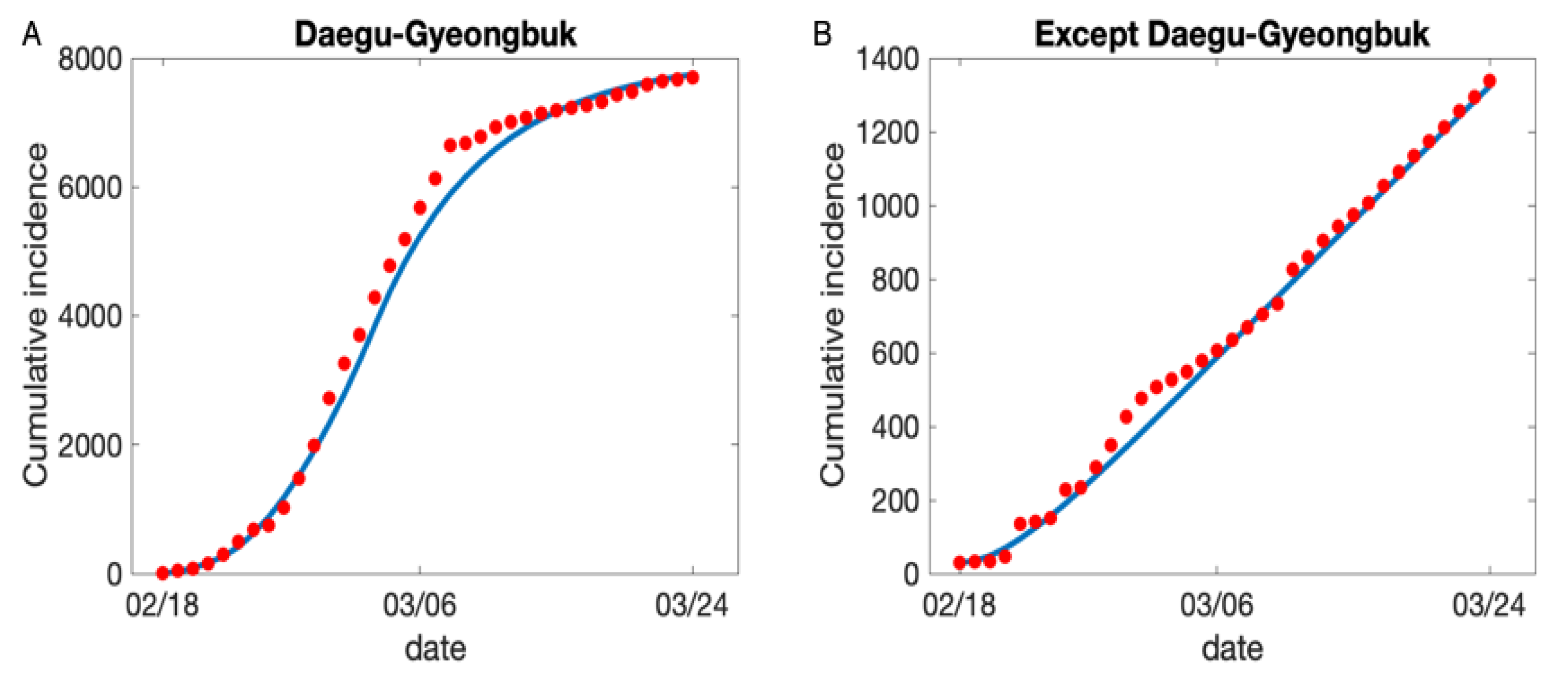
3. Parameter Estimation

3.1. Estimated Parameter

As shown in Figure 2, the daily confirmed cases of COVID-19 in the Daegu and Gyeongbuk area show special features; the number of confirmed cases demonstrated a slow initial increase at the beginning, shortly after the 31st confirmed case, a rapid increase of cases. After the peak of confirmed cases, the number of cumulative incidences remained steady (almost no increase). To capture this special feature, the entire time interval ([0, 40] days) was divided into the following 3 subintervals: a small increase interval $[t_0,t_1)$, a rapid increase interval $[t_1,t_2)$, and a slower increase interval $[t_2,t_{end})$. Therefore, we estimated three different transmission rates, a small ${\beta }_{1,1}$ during $[t_0,t_1)$, a rapid increase with a transmission rate ${\beta }_{1,2}$ during time $[t_1,t_2)$, and a slower increase of incidence after peak with a transmission rate ${\beta }_{1,3}$ during $[t_1,t_{end})$ ( ${\beta }_{1,3}<{\beta }_{1,1}<{\beta }_{1,2}$).

We set the initial susceptible population to be 5.12 million and 46.52 million in the Daegu and Gyeongbuk and the rest of Korea, respectively (ie, $S_1\left(t_0\right)=5.12\times {10}^6\&S_2\left(t_0\right)=46.52\times {10}^6$) as the population size of the two patches. The initial quarantine numbers of $Q_{1,2}\left(t_0\right)$ were taken from the cumulative incidence data on 18 February 2020. We assumed the number of exposed $E_{1,2}\left(t_0\right)$ and recovered $R_{1,1}\left(t_0\right)$ to be zero. The number of initially infected individuals ($I_{1,2}\left(t_0\right)$) was not measurable and thus was estimated using the method below.

Using the report by Workman [36], we set the percentage of asymptomatic individuals to be 33.3% (i.e., $p=0.333$). To estimate a typical number of traveling in Korea, we used data from the 2016 Korea Transport Data Base, a national organization that produces, manages, and provides various transportation data for Korea (KOTI) [30]. The remaining 10 parameters and 2 initial numbers of infected $\left(I_{1,2}\left(t_0\right)\right)$ were estimated. An inverse least-squares formulation was used to find a parameter set ($\theta$) that minimized the least-squares error between cumulative incidence of the model outputs ($C_{1,2}$) and actual cumulative incidence data ($D_{1,2}$) from 18 February to 24 March 2020.

The least-squares error J is defined as

$$J\left(\theta \right)=\sqrt{{\sum }_{j=1}^N{\left(C_1(t_j,y\left(t_j\right);\theta )-D_1\left(t_j\right)\right)}^2+{\sum }_{j=1}^N{\left(C_2(t_j,y\left(t_j\right);\theta )-D_2\left(t_j\right)\right)}^2},$$

(6)

where $\theta$ represents a set of parameters, $t_j$ time points (with $j=1,\cdots ,N$), and $D_{1,2}$ actual cumulative incidence data (a subscript denotes a patch; $C_1,D_1$ for patch 1 and $C_2,D_2$ for patch 2). The optimal parameter set is given by

$$\widehat{\theta }=\underset{\theta }{arg\; min}J\left(\theta \right).$$

(7)

We used the Nelder–Mead simplex method [38], which aims to minimize the least-squares error through a direct search using MATLAB’s built-in optimization function fminsearch. The optimal parameter values for the two-patch model are given in Table 2, and the fitted curves generated by the estimated parameters are shown in Figure 5. Cumulative incidence of the two-patch model (solid blue curve) and COVID-19 data (red circles) in each patch are in good agreement.

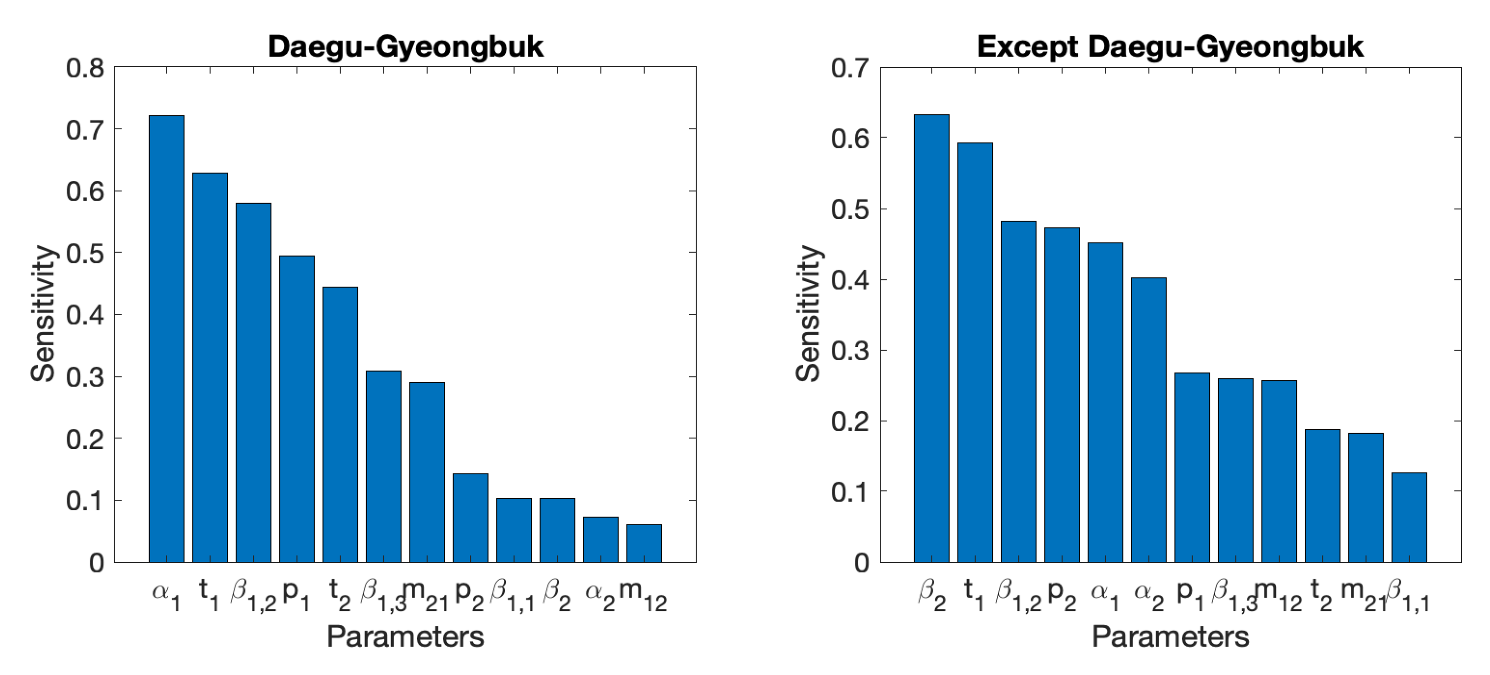
3.2. Sensitivity Analysis

To assess the variation of the model outputs in response to small perturbations in the parameter values, we performed a global sensitivity analysis that described how a model output changed in response to varying the parameters over a subspace of the parameter space. A global sensitivity method developed by [39] is a variance decomposition method. First, input parameters are varied, which causes model output to be varied. Next, the variance of the model output is quantified. Then, a partial variance is calculated by partitioning of model output variance to determine what fraction of the model output variance is caused by the variation of each model parameter input.

The model outputs we considered were $C_1$, cumulative incidences in the Daegu and Gyeongbuk, and $C_2$, cumulative incidences in the rest of Korea except for Daegu and Gyeongbuk. The sensitivity indices computed by the method described in [39] are shown in Figure 6. The left panel for patch 1 shows various sensitivity analysis; the model output $C_1$ was highly sensitive to the parameters ${\alpha }_1,t_1,{\beta }_{1,2},p_1,t_2$, where ${\alpha }_1$ indicates a detection rate from $I_1$ to $Q_1$, and ${\beta }_{1,2}$ represents a transmission rate during $(t_1,t_2)$, while $p_1$ is a proportion from $E_1$ to $I_1$.

Next, the right panel for patch 2 shows various sensitivity analysis; the model output $C_2$ was highly sensitive to the parameters ${\beta }_2,t_1,{\beta }_{1,2},p_2,{\alpha }_1,{\alpha }_2$, where ${\beta }_2$ indicates a transmission rate of patch 2, $t_1$ represents the time when a rapid increase of incidences was observed in the Daegu/Gyeongbuk area, ${\beta }_{1,2}$ is a transmission rate during $(t_1,t_2)$ in the Daegu/Gyeongbuk area, $p_2$ indicates a proportion from $E_2$ to $I_2$, and ${\alpha }_{1,2}$ represents a detection rate from $I_{1,2}$ to $Q_{1,2}$, respectively. Cumulative incidence in patch 1, $C_1$ is sensitive to $m_{21}$ (mobility from patch 2 to patch 1) while cumulative incidence in patch 2, $C_2$ is sensitive to $m_{12}$ (mobility from patch 1 to patch 2).

4. Numerical Simulations

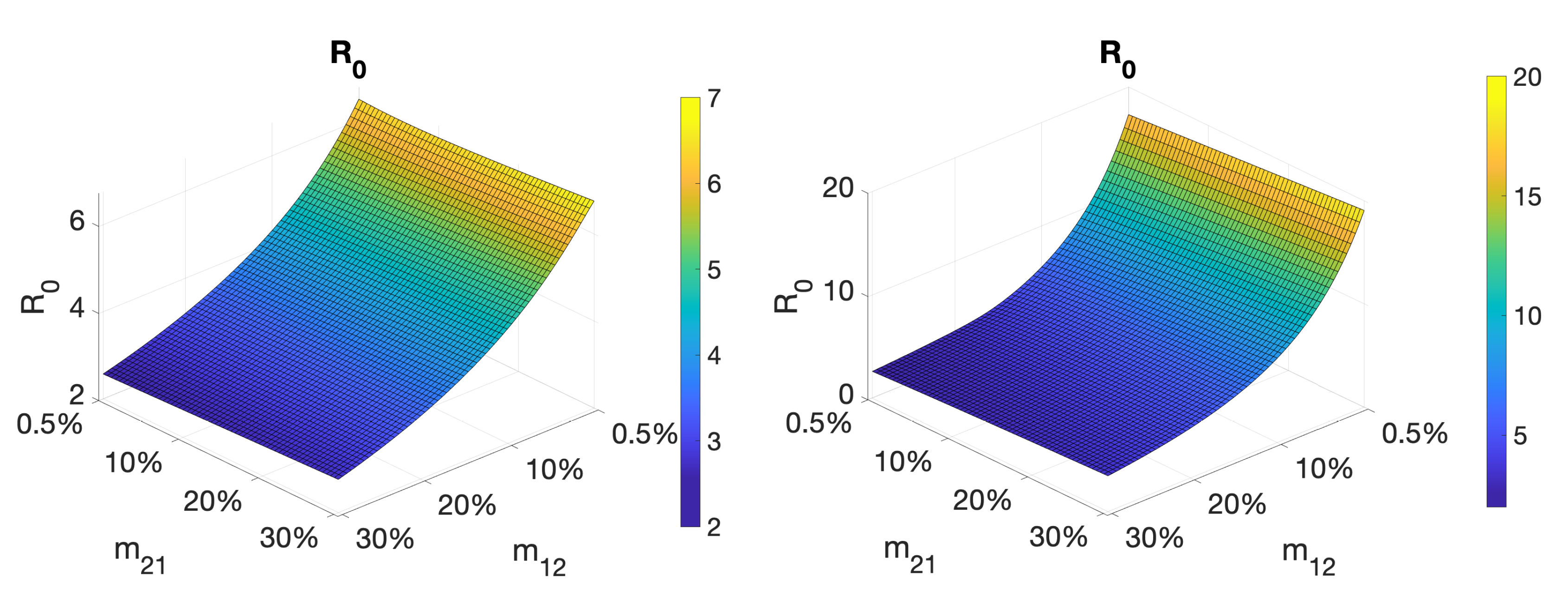
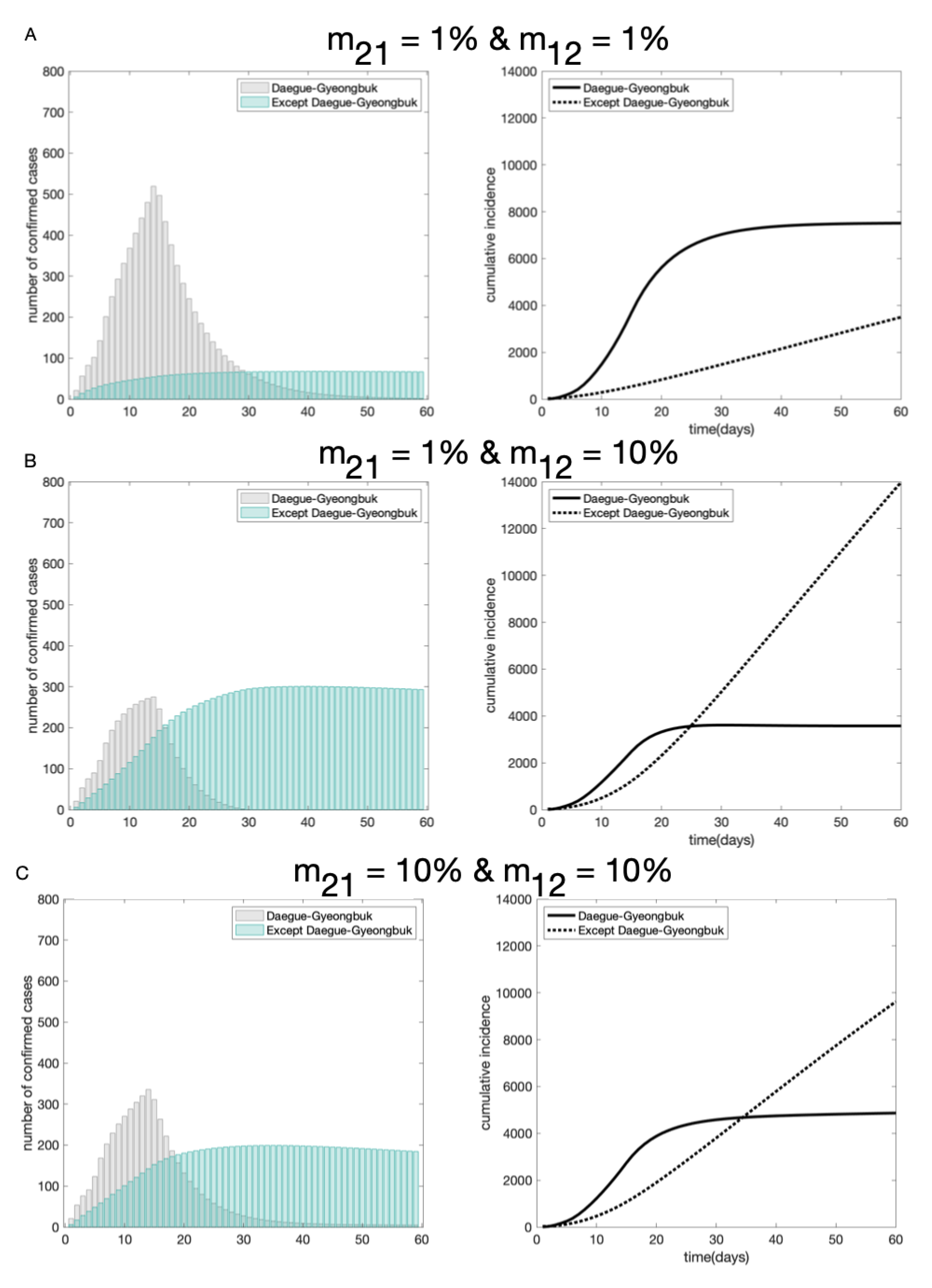
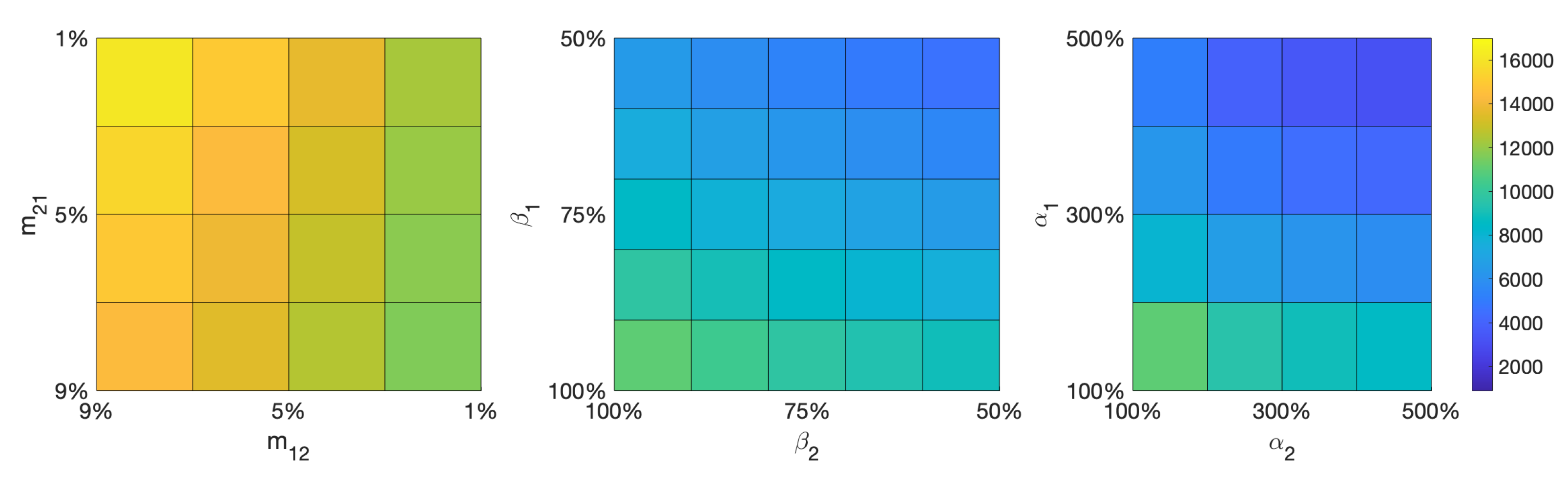
4.1. The Impact of Mobility on the COVID-19 Transmission Dynamics

First, we investigate the impacts of movement (travel or mobility) on the two-patch transmission dynamics: Daegu and Gyeongbuk (the epicenter) are represented by patch 1 and the rest of Korea is patch 2. Other parameters are fixed as the baseline parameter values given in Table 2. The average number of travelers between the two areas was obtained from the Korea Transport DataBase in 2016 [30] ($m_{12}$ and $m_{21}$ are given in Table 2). In 2016, the average number of people traveling was 1.9 million per day, however, the average daily nationwide level of traffic for the first three months of 2020 was 9.7% lower than the same period in 2019. After the alert level of COVID-19 raised to the highest level on 22 February 2020, traffic in the 4th week of February was down by 26.1% compared with the one of 2019 [40].

We assume that a reduction (0.5–30%) of the average number of mobility to mimic the travel reduction due to the COVID-19 outbreak. Now, we present the impact of mobility on the global $R_0$ given in (5) under the range (0.5–30%) of the average number in $m_{12}$ and $m_{21}$. In Figure 7, the global $R_0$ is displayed as a function of $m_{12}$ and $m_{21}$. The left panel shows the global $R_0$ (lower) using the transmission rate ${\beta }_1=0.338$ in Daegu and Gyeongbuk & transmission rate ${\beta }_2=0.357$ in the rest of Korea. The right panel shows the global $R_0$ (higher) with the transmission rate ${\beta }_1=0.9$ in Daegu and Gyeongbuk and a transmission rate ${\beta }_2=0.357$ in the rest of Korea. Interestingly, the global $R_0$ gets larger as less people traveled from the epicenter to the rest of Korea (or people stay more in Daegu and Gyeongbuk). The increase was more dramatic when the transmission rate in the epicenter was higher (right). A previous study also reported similar simulation results [14], arguing that this is a result of the dilution effect (people move more than COVID-19 spread from the epicenter to other areas).

Next, we present the impacts of mobility on daily and cumulative incidence in the two patches as migration rate changes from 1% to 10% (see Figure 8). The top panel shows the baseline results under $m_{12}=m_{21}=1\%$. The peak size of daily incidences and cumulative confirmed cases in patch 1 was highest (519 cases and 7821 cases, respectively). The number of confirmed cases in the rest of Korea remained relatively small (peak, 67 cases; cumulative incidences, 3497 cases) as the actual COVID outbreak with the highest spatial heterogeneity.

The middle panel shows the results under $m_{12}=10\%,m_{21}=1\%$, which implies that more people were traveling out of the Daegu and Gyeongbuk to the rest of Korea. We observed a decrease in the confirmed cases (approximately a 50% reduction) in the Daegu and Gyeongbuk, whilst a sharp increase in cases was expected (∼400%) in the rest of Korea (Figure 8; the first panel vs. the second panel).

Interestingly, increases in traveling between the two areas (epicenter and the rest of Korea) resulted in a reduced number of confirmed cases in the epicenter, as shown in the bottom panel under $m_{12}=10\%,m_{21}=10\%$. It turns out that travel restrictions from Daegu and Gyeongbuk to other areas prevented the spread of COVID-19 across the whole country.

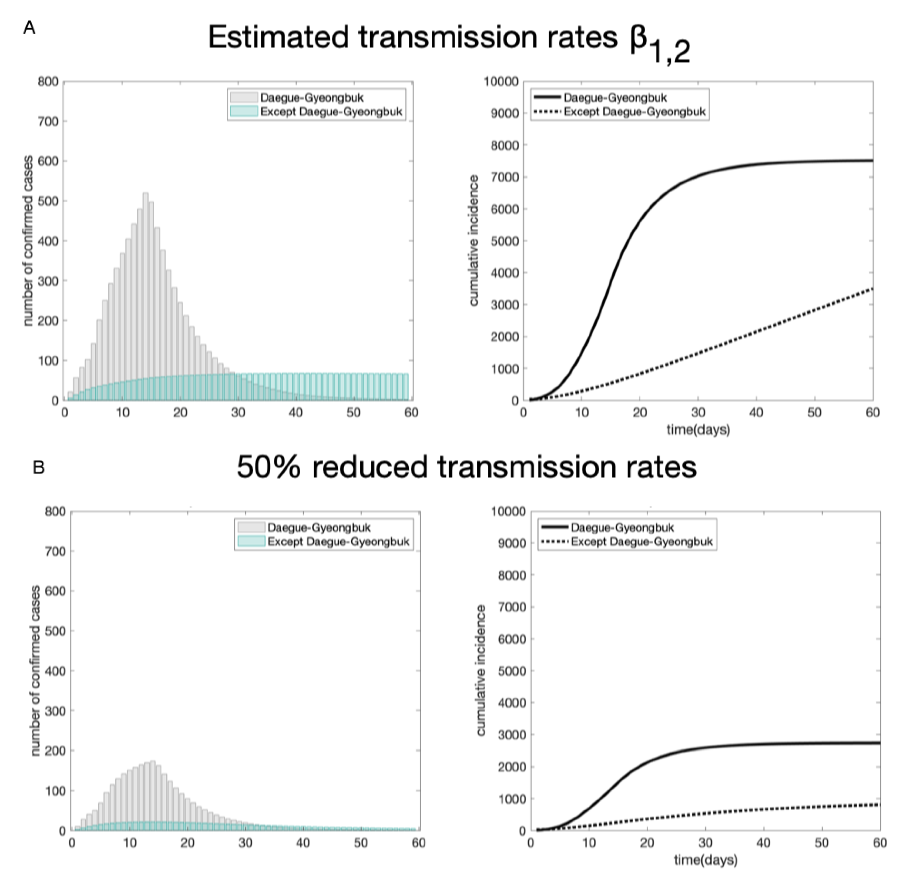
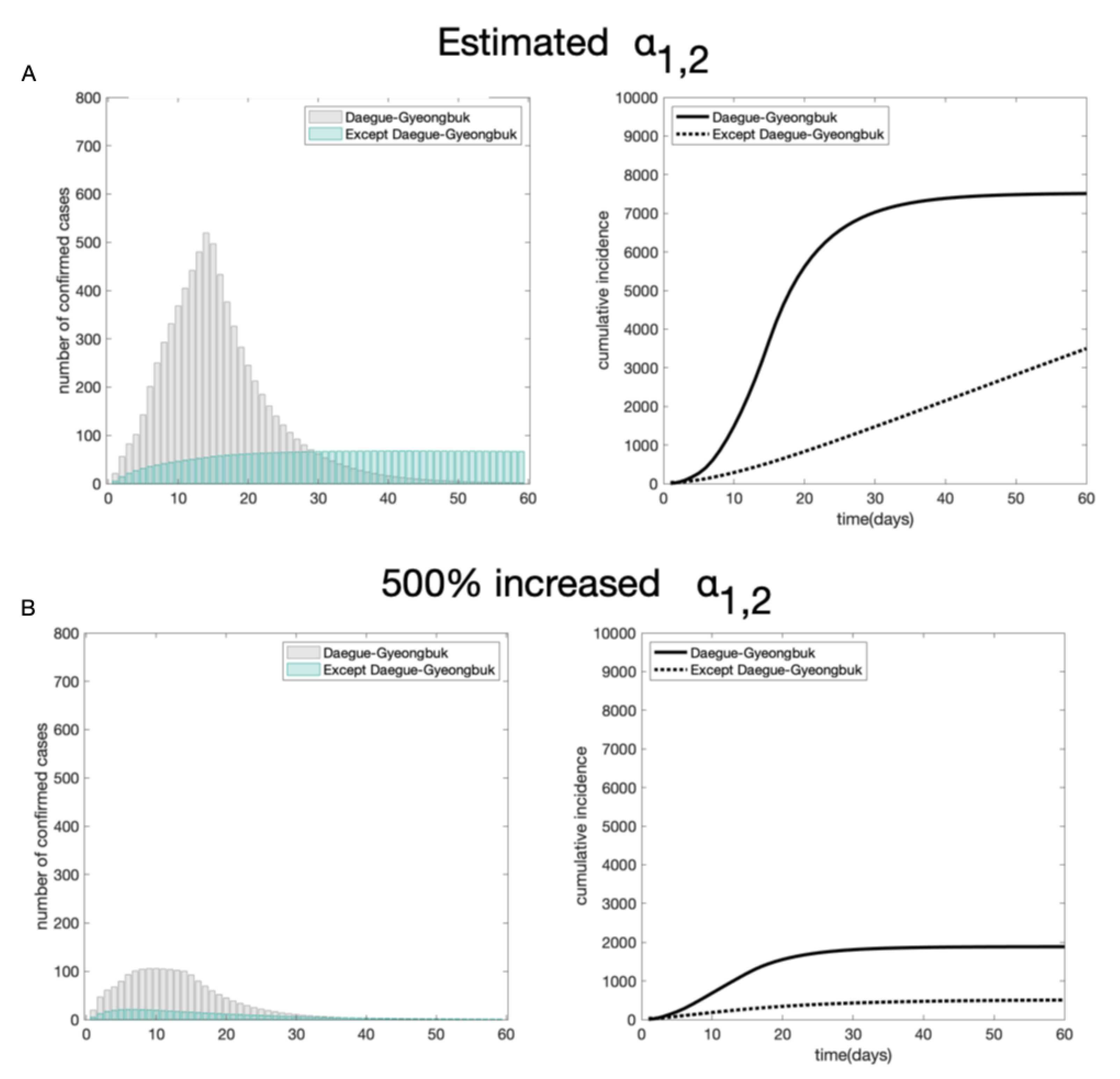
4.2. The Impact of Social Distancing and Early Detection on the COVID-19 Transmission Dynamics

In this subsection, we explore the impacts of two other interventions (social distancing and early detection) on two-patch COVID-19 transmission dynamics. Assuming minimal levels of travel between the two areas (epicenter and the rest of Korea), we evaluated the impacts of social distancing and early detection on the patch-specific peak size and cumulative incidence. Social distancing was simply modeled by reducing the transmission rate, $\sigma {\beta }_i$, $i=1,2$ with $\sigma =0.5$, where ${\beta }_i$ was an estimated value and given in Table 2. Figure 9 shows the effects of $\sigma {\beta }_i$ on patch-specific incidence of COVID-19 under two different combinations of $\sigma {\beta }_i$, $i=1,2$. The top panel shows the results under the baseline scenarios as given in Table 2, and the bottom panel shows the results assuming 50% reduced transmission rates. Halved transmission rates (50% reduction) led to an approximate 67% reduction in the spread in the two areas, respectively. This is consistent with the results of the global sensitivity analysis (patch-specific cumulative incidence was the most sensitive to the transmission rates in patch 2, as shown in Figure 6).

Next, we investigate the impact of early detection on two-patch COVID-19 transmission dynamics. What if asymptomatic patients were efficiently traced, identified, and quarantined? To address this question, we simulated community spread increasing the estimated model parameters ${\alpha }_{1,2}$. The early detection was modeled by incorporating a re-scaling constant, $\eta$ in the rate, $\eta {\alpha }_i$, $i=1,2$ with $\eta =[1,500]$, where the estimated ${\alpha }_1$ was 0.031 in the epicenter while the value was 0.35 in the rest of Korea. Figure 10 shows the effects of $\eta {\alpha }_i$ on the patch-specific incidence of COVID-19 under two different combinations of $\eta {\alpha }_i$, $i=1,2$. The top panel shows the results under $\eta =1$ and the baseline scenarios given in Table 2. The bottom panel shows the results when the early detection rate was increased. Five hundred-fold increases of ${\alpha }_{1,2}$ resulted in an approximate 70% reduced spread in each area. Taken together, the identification of asymptomatic individuals by extensive testing contributed to controlling massive outbreaks. This is consistent with the results of the global sensitivity analysis (patch-specific cumulative incidence was the most sensitive to the early detection rates in patch 1, as shown in Figure 6).

5. Discussion

In this work, we developed a single-patch and a two-patch model for COVID-19 transmission dynamics, focusing on the largest outbreak in Daegu and Gyeongbuk and the rest of South Korea. We investigate the impacts of three different intervention strategies on the COVID-19 transmission dynamics. These include travel restrictions, social distancing, and the efficient early detection of confirmed cases followed by quarantine.

First, travel restrictions are particularly useful in the early stage of the COVID-19 outbreak confined to a certain area. However, travel restrictions may be less effective once the outbreak is more widespread [23]. Our simulations showed that travel restrictions delayed the spread of the disease into the rest of Korea from the epicenter and reduced the number of total incidences (see the leftmost panel of Figure 11, 12,000 cases at 1% vs 16,000 cases at 9%). An increased travel movement between Daegu and Gyeongbuk and the rest of Korea resulted in a reduced number of confirmed cases in the epicenter but not in the rest of Korea. The travel ban in Wuhan and the international travel restrictions did not show noticeable differences in the epidemic in Wuhan but delayed ∼3 days for other locations in mainland China [24]. Another study demonstrated that internal mobility restrictions are effective only if prohibitively high ($50\%$ of travel) restrictions are applied [26]. In another infection study, Ref. [41] suggested that short-term mobility between heterogeneous patches does not always contribute to overall increases in the prevalence of tuberculosis. In [14], the strategy of the migration restriction may result in locally bigger outbreaks rather than extinguishing the pandemic spread, even though the spread is delayed. Our results are consistent with other studies showing that travel restrictions may not be particularly effective to reduce the cumulative incidence.

Second, social distancing measures aim to reduce the frequency of contact, and increase the physical distance between individuals, reducing the risks of person-to-person transmission. A large number of published studies examining social distancing conducted during the 2009 influenza pandemic concluded that social distancing controlled the epidemic [26]. Data-driven models of COVID-19 spread in China [27] have shown that strict social distancing for 30 days had significant benefits in limiting community spread Wuhan and Hubei. Choi et al suggested that social distancing is crucial in suppressing the spread of the COVID-19 in Korea [28]. Furthermore, the transmission of viruses was lower with the physical distancing of 1 meter or more, compared with a distance of less than 1 m [25]. Our simulations also showed that strict social distancing led to a significant reduction in total incidences. Approximately 2000 fewer cases were expected as transmission rates were decreased by 10% (see the middle panel of Figure 11). From 12 April to 18 April, after four weeks of strict social distancing was enforced, the number of confirmed cases decreased dramatically [8]. In the situation of a lack of therapeutics and without vaccines, social distancing is one of the basic protective measures against COVID-19.

Lastly, one of the notable things about COVID-19 is the high rate of asymptomatic but infectious individuals. In Korea, approximately 33.3% of the confirmed cases were asymptomatic [36]. In Italy, $42.5\%$ of the confirmed infections detected were asymptomatic [42]. Thus, identification of asymptomatic virus carriers by aggressive testing and contact tracing could potentially reduce the size of the epidemic. Our simulations varying the detection rate $\alpha$ suggested that approximately 2000 confirmed cases (approximately 20% of the total incidence) could be reduced by doubling detection rates (see the rightmost panel of Figure 11). Another study also demonstrated that the identification of undocumented COVID-19 cases suppressed the spread of COVID-19 [4]. Early detection is also a necessary method for preventing transmission. To mitigate the spread of the disease, it is important to detect the outbreak of the patient early, conduct quarantine and treatment, and identify contacts through effective epidemiological surveillance systems and investigations.

6. Conclusions

We have investigated the COVID-19 transmission dynamics using a two-patch SEIQR system with a mobility matrix. The two patches represent the epicenter (Daegu/Gyeongbuk) and the rest of Korea to capture two distinct characteristics of COVID-19 outbreaks with the highest spatial heterogeneity. Some of the essential epidemic parameters including patch-specific transmission rates and the local and global $R_0$ have been estimated using empirical cumulative incidence data of COVID-19 from 18 February to 24 March 2020. We have investigated the impacts of several interventions implemented by the Koran government including travel restrictions, social distancing, and early diagnostic interventions. Our results indicate that the two-patch dynamics are strongly dependent on the following three key factors: mobility, transmission rates, early diagnostic interventions. Overall, implementing all possible interventions together would be the most effective in controlling the COVID-19 outbreaks, however, that would increase the higher economic burden and social costs as well. The present study focused only on the first two months of COVID-19 outbreaks, and we would like to extend our work to a multi-city model, which can capture the entire course of COVID-19 transmission in South Korea for our future study.

References

1. Mayo Clinic. Available online: https://www.mayoclinic.org/diseases-conditions/coronavirus/symptoms-causes/syc-20479963 (accessed on 27 May 2020).
2. Verity, R.; Okell, L.C.; Dorigatti, I.; Winskill, P.; Whittaker, C.; Imai, N.; Cuomo-Dannenburg, G.; Thompson, H.; Walker, P.; Fu, H.; et al. Estimates of the severity of COVID-19 disease. medRxiv 2020. [Google Scholar] [CrossRef]
3. Center for Disease Control (CDC). Available online: https://www.cdc.gov/coronavirus/2019-ncov/symptoms-testing/symptoms.html (accessed on 27 May 2020).
4. Li, R.; Pei, S.; Chen, B.; Song, Y.; Zhang, T.; Yang, W.; Shaman, J. Substantial undocumented infection facilitates the rapid dissemination of novel coronavirus (SARS-CoV2). Science 2020, 6490, 489–493. [Google Scholar] [CrossRef] [Green Version]
5. World Health Organization(WHO). Coronavirus. Available online: https://www.who.int/emergencies/diseases/novel-coronavirus-2019/situation-reports (accessed on 31 March 2020).
6. Johns Hopikins University and Medicine. Coronavirus Resource Center. Available online: https://coronavirus.jhu.edu/map.html (accessed on 31 March 2020).
7. The Korea Herald. Available online: http://www.koreaherald.com/view.php?ud=20200305000889$&$np=85$&$mp=9 (accessed on 6 March 2020).
8. Korea Center for Disease Control (KCDC). Available online: https://www.cdc.go.kr/board/ (accessed on 2 March 2020).
9. Brauer, F.; Castillo-Chavez, C. Mathematical Models in Population Biology and Epidemiology; Springer: New York, NY, USA, 2000. [Google Scholar]
10. Murray, J.D. Mathematical Biology. II: Spatial Models and Biomedical Applications; Springer: Berlin/Heidelberg, Germany, 2003. [Google Scholar]
11. Sattenspiel, L.; Dietz, K. A structured epidemic model incorporating geographic- mobility among regions. Math. Biosci. 1995, 128, 71–91. [Google Scholar] [CrossRef]
12. Lee, S.; Castillo-Chavez, C. The Role of Residence Times in Two-Patch Dengue Transmission Dynamics and Optimal Strategies. J. Theor. Biol. 2015, 374, 152–164. [Google Scholar] [CrossRef]
13. Hyman, J.M.; Laforce, T. Modeling the Spread of Influenza Among Cities. In Biomathematical Modeling Applications in Homeland Security; SIAM: Philadelphia, PA, USA, 2003. [Google Scholar]
14. Lee, J.M.; Choi, D.; Cho, G.; Kim, Y. The effect of public health interventions on the spread of influenza among cities. J. Theor. Biol. 2012, 293, 131–142. [Google Scholar] [CrossRef]
15. Anastassopoulou, C.; Russo, L.; Tsakris, A.; Siettos, C. Data-Based Analysis, Modelling and Forecasting of the novel Coronavirus (2019-nCoV) outbreak. medRxiv 2020. [Google Scholar] [CrossRef]
16. Yang, Y.; Lu, Q.; Liu, M.; Wang, Y.; Zhang, A.; Jalali, N. Epidemiological and clinical features of the 2019 novel coronavirus outbreak in China. medRxiv 2020. [Google Scholar] [CrossRef] [Green Version]
17. You, C.; Deng, Y.; Hu, W.; Sun, J.; Lin, Q.; Zhou, F. Estimation of the Time-Varying Reproduction Number of COVID-19 Outbreak in China. Int. J. Hyglene Environ. Health 2020. [Google Scholar] [CrossRef]
18. Mizumoto, K.; Kagaga, K.; Chowell, G. Early epidemiological assessment of the transmission potential and virulence of 2019 Novel Coronavirus in Wuhan City: China, 2019. medRxiv 2020. [Google Scholar] [CrossRef] [Green Version]
19. Wu, J.; Leung, K.; Leung, G. Now casting and forecasting the potential domestic and international spread of the 2019-nCoV outbreak originating in Wuhan, China: A modelling study. Lancet 2020, 395, 689–697. [Google Scholar] [CrossRef] [Green Version]
20. Kucharski, A.J.; Russell, T.W.; Diamond, C.; Liu, Y.; Edmunds, J.; Funk, S.; Eggo, R.M.; Sun, F.; Jit, M.; Munday, J.D.; et al. Early dynamics of transmission and control of 2019-nCoV: A mathematical modelling study. medRxiv 2020. [Google Scholar] [CrossRef]
21. Piccolomiini, E.L.; Zama, F. Monitoring Italian COVID-19 spread by an adaptive SEIRD model. medRxiv 2020. [Google Scholar] [CrossRef] [Green Version]
22. Sadun, L. Effects of Latency on Estimates of the COVID-19 Replication Number. Bull. Math Biol. 2020, 82, 114. [Google Scholar] [CrossRef] [PubMed]
23. Kraemer, M.U.; Yang, C.H.; Gutierrez, B.; Wu, C.H.; Klein, B.; Pigott, D.M.; Du Plessis, L.; Faria, N.R.; Li, R.; Hanage, W.P.; et al. The effect of human mobility and control measures on the COVID-19 epidemic in China. Science 2020, 6490, 493–497. [Google Scholar] [CrossRef] [Green Version]
24. Chinazzi, M.; Davis, J.T.; Ajelli, M.; Gioannini, C.; Litvinova, M.; Merler, S.; Piontti, A.P.; Mu, K.; Rossi, L.; Sun, K.; et al. The effect of travel restrictions on the spread of the 2019 novel coronavirus (COVID-19) outbreak. Science 2020, 6489, 395–400. [Google Scholar] [CrossRef] [PubMed] [Green Version]
25. Chu, D.K.; Akl, E.A.; Duda, S.; Solo, K.; Yaacoub, S.; Schünemann, H.J.; El-harakeh, A.; Bognanni, A.; Lotfi, T.; Loeb, M.; et al. Physical distancing, face masks, and eye protection to prevent person-to-person transmission of SARS-CoV-2 and COVID-19: A systematic review and meta-analysis. Lancet 2020, 395, 1973–1987. [Google Scholar] [CrossRef]
26. Rashid, H.; Ridda, I.; King, C.; Begun, M.; Tekin, H.; Wood, J.G.; Booy, R. Evidence Compendium and Advice on Social Distancing and Other Related Measures for Response to an Influenza Pandemic. Paediatr. Respir. Rev. 2015, 16, 119–126. [Google Scholar] [CrossRef] [PubMed]
27. Zhang, Y.; Jiang, B.; Yuan, J.; Tao, Y. The impact of social distancing and epicenter lockdown on the COVID-19 epidemic in mainland China: A data-driven SEIQR model study. medRxiv 2020. [Google Scholar] [CrossRef]
28. Choi, S.; Ki, M. Estimating the reproductive number and the outbreak size of COVID-19 in Korea. Epidemiol. Health 2020, 42, e2020011. [Google Scholar] [CrossRef]
29. Ryu, S.; Ali, S.T.; Jang, C.; Kim, B.; Cowling, B.J. Effect of Nonpharmaceutical Interventions on Transmission of Severe Acute Respiratory Syndrome Coronavirus 2, South Korea, 2020. Emerg. Infect. Dis. 2020, 26, 2406. [Google Scholar] [CrossRef]
30. Korea Transfortation DataBase. Available online: https://www.ktdb.go.kr (accessed on 15 May 2020).
31. KCDC Briefing Report. Available online: http://ncov.mohw.go.kr/tcmBoardList.do?brdId=3&brdGubun= (accessed on 22 March 2020).
32. Daegu Briefing Report. Available online: https://www.daegu.go.kr/icms/bbs/selectBoardArticle.do (accessed on 28 February 2020).
33. van den Driessche, P.; Watmough, J. Reproduction numbers and sub-threshold endemic equilibria for compartmental models of disease transmission. Math. Biosci. 2002, 180, 29–48. [Google Scholar] [CrossRef]
34. Coronavirus Incubation Period: 2–14 days. Available online: https://www.worldometers.info/coronavirus/coronavirus-incubation-period/ (accessed on 12 March 2020).
35. Byrne, A.W.; McEvoy, D.; Collins, A.; Hunt, K.; Casey, M.; Barber, A.; Butler, F.; Griffin, J.; Lane, E.; McAloon, C.; et al. Inferred duration of infectious period of SARS-CoV-2: Rapid scoping review and analysis of available evidence for asymptomatic and symptomatic COVID-19 cases. BMJ Open 2020, 10, e039856. [Google Scholar] [CrossRef]
36. Workman, J. Proportion of COVID-19 Cases that Are Asymptomatic in South Korea: Comment on Nishiura et al. Int. J. Infect. Dis. 2020, 96, 398. [Google Scholar] [CrossRef] [PubMed]
37. Korean Statistical Information Service. Available online: http://kosis.kr (accessed on 15 May 2020).
38. Seber, G.A.F.; Wild, C.J. Nonlinear Regression; John Wiley & Sons, Inc.: Hoboken, NJ, USA, 2003. [Google Scholar]
39. Marino, S.; Hogue, I.B.; Ray, C.J.; Kirschner, D. E A methodology for performing global uncertainty and sensitivity analysis in systems biology. J. Theor. Biol. 2008, 254, 178–196. [Google Scholar] [CrossRef] [PubMed] [Green Version]
40. Lee, H.; Park, S.J.; Lee, G.R.; Kim, J.E.; Lee, J.H.; Jung, Y.; Nam, E.W. The relationship between trends in COVID-19 prevalence and traffic levels in South Korea. Int. J. Infect. Dis. 2020, 96, 399–407. [Google Scholar]
41. Moreno, V.; Espinoza, B.; Barley, K.; Paredes, M.; Bichara, D.; Mubayi, A.; Castillo-Chavez, C. Role of Mobility and Health Disparities on the Transmission Dynamics of Tuberculosis. Theor. Biol. Med. Model. 2017, 14, 3. [Google Scholar] [CrossRef] [PubMed]
42. Lavezzo, E.; Franchin, E.; Ciavarella, C.; Cuomo-Dannenburg, G.; Barzon, L.; Del Vecchio, C.; Rossi, L.; Manganelli, R.; Loregian, A.; Navarin, N.; et al. Suppression of a SARS-CoV-2 outbreak in the Italian municipality of Vo’. Nature 2020, 584, 425–429. [Google Scholar] [CrossRef] [PubMed]
Figure 1. The spatial distribution of cumulative incidence is displayed in the South Korea map; a total of 10,512 confirmed cases in South Korea and 8217 confirmed cases in Daegu and Gyeongbuk as of 29 April 2020.
Processes 08 01304 g001
Figure 2. The time series of daily incidence in Daegu and Gyeongbuk (grey bar) is compared with the daily incidence in the rest of South Korea (green bar). Administrative countermeasures are implemented by the Korean government (Daegu and Gyeongbuk).
Processes 08 01304 g002
Figure 3. The flow chart of a single-patch model for COVID-19 transmission dynamics is displayed.
Processes 08 01304 g003
Figure 4. The flow chart of a two-patch model for COVID-19 transmission dynamics is displayed; patch 1 represents Daegu and Gyeongbuk and patch 2 represents the rest of South Korea.
Processes 08 01304 g004
Figure 5. (A) Model calibration to Daegu-Gyeongbuk incidence data (blue solid line: model prediction, red dots: data. (B) Model calibration to South Korea incidence data except Daegu-Gyeongbuk area.
Processes 08 01304 g005
Figure 6. A global sensitivity analysis is displayed; left panel of patch 1 and right panel of patch 2 under various patch-specific parameters.
Processes 08 01304 g006
Figure 7. Effect of mobility ( m i j ) on the global R 0 . The global R 0 is displayed as a function of m 12 and m 21 . The left panel with the transmission rate β 1 = 0.338 in Daegu and Gyeongbuk and a transmission rate β 2 = 0.357 in the rest of Korea. The right panel with the transmission rate β 1 = 0.9 in Daegu and Gyeongbuk and a transmission rate β 2 = 0.357 in the rest of Korea.
Processes 08 01304 g007
Figure 8. The impact of different motility on daily incidences and cumulative incidence. (A) 1% of population is traveling between two patches. (B) 1% of population in patch 2 migrates to the patch 1, while 10% of population in patch 1 migrates to the patch 2. (C) 10% of population in both patches are traveling between two patches.
Processes 08 01304 g008
Figure 9. The impacts of different social distancing on daily incidences and cumulative incidences. (A) Effect of not strict social distancing assuming estimated transmission rates on the incidences. (B) Effect of more strict social distancing assuming 50% of transmission rates on the incidences.
Processes 08 01304 g009
Figure 10. The impact of different early detection rate on daily incidences and cumulative incidences. (A) Early detection rate is assumed as estimated α 1 , 2 . (B) The effect of 5 fold increase of the detection rate on the incidences.
Processes 08 01304 g010
Figure 11. The impacts of three different patch-specific interventions on cumulative incidence are shown; the leftmost panel of travel restriction, the middle panel of social distancing, the rightmost panel of early detection rate (measured at day 60).
Processes 08 01304 g011