Nexus between Energy Usability, Economic Indicators and Environmental Sustainability in Four ASEAN Countries: A Non-Linear Autoregressive Exogenous Neural Network Modelling Approach

 , , and
Abstract
:1. Introduction
2. Materials and Methods
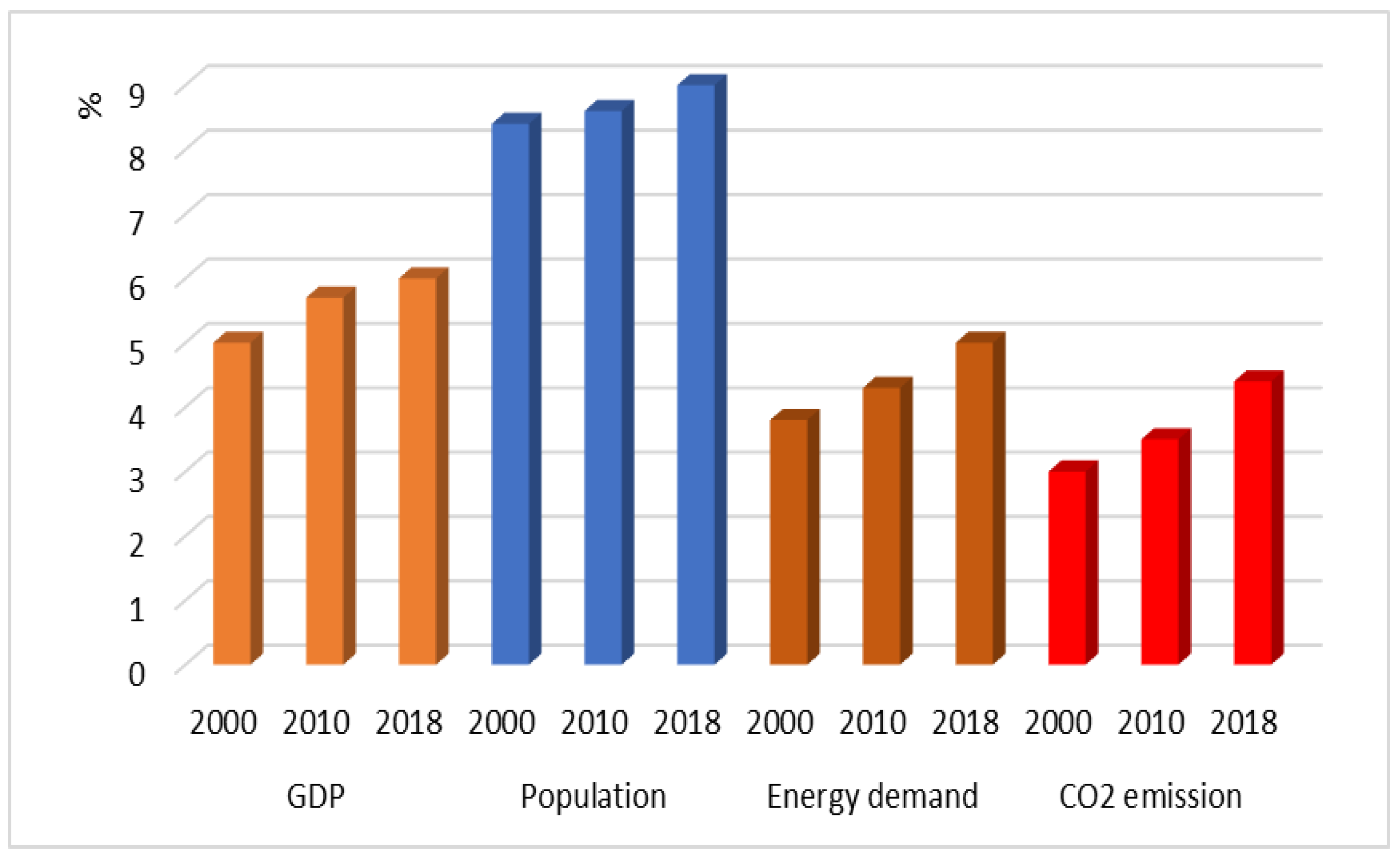
2.1. Data Description
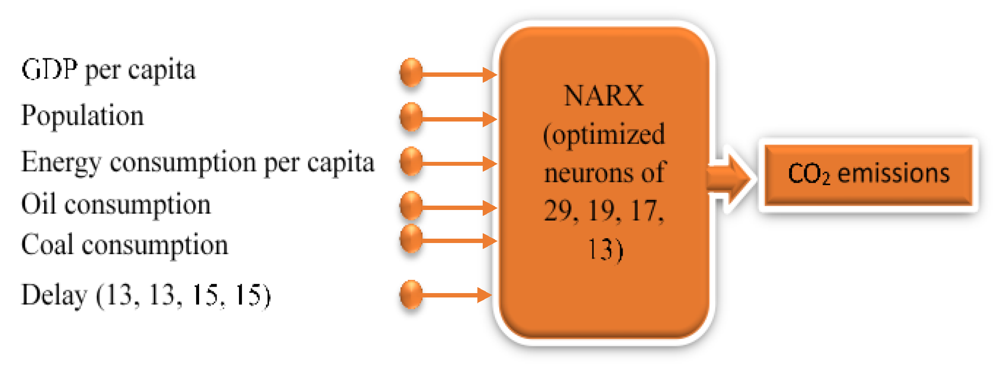
2.2. The NARX Neural Network Modelling
2.3. Sensitivity Analysis of the Input Variables
3. Results and Discussion
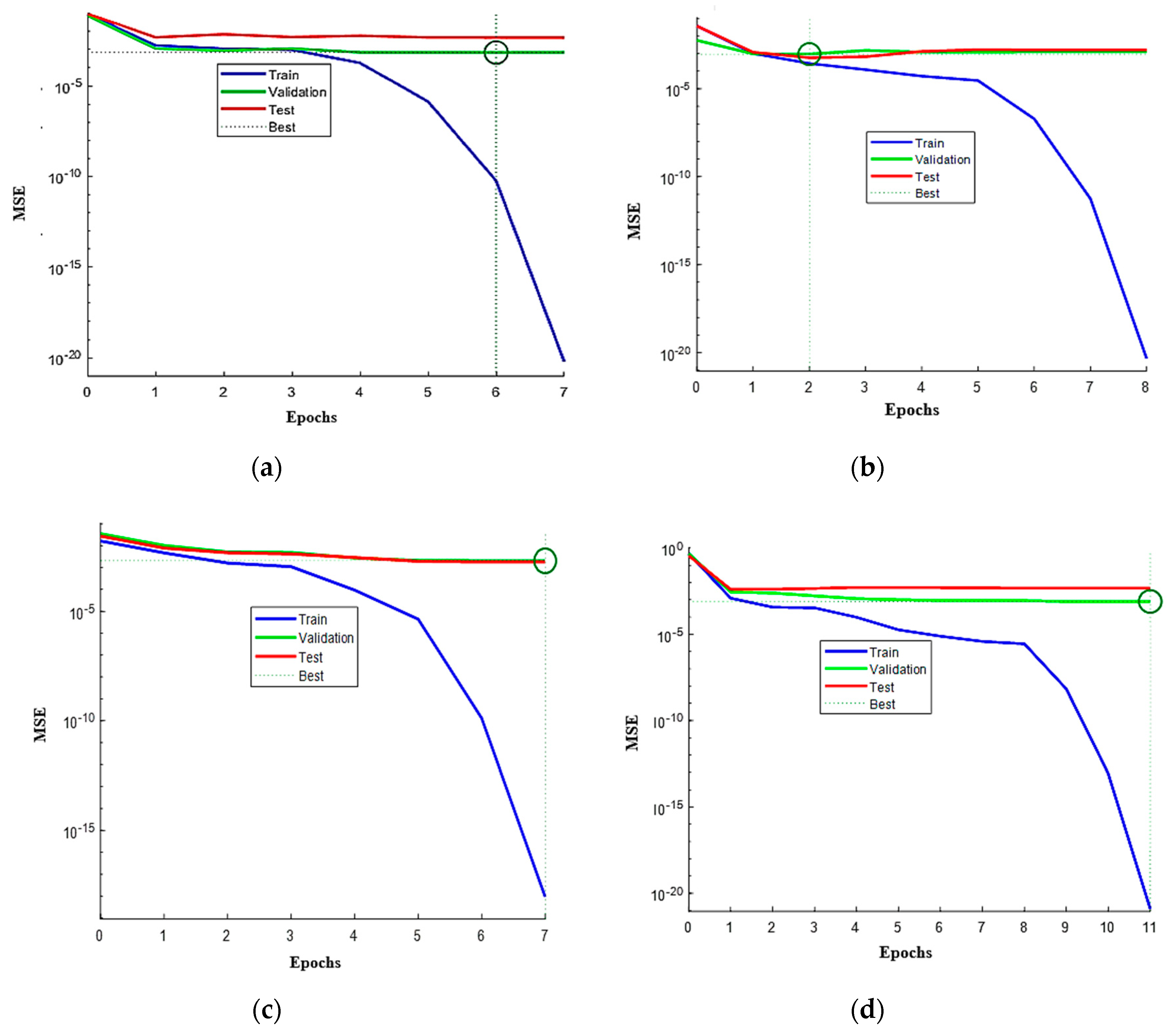
3.1. Optimization of the Hidden Neurons
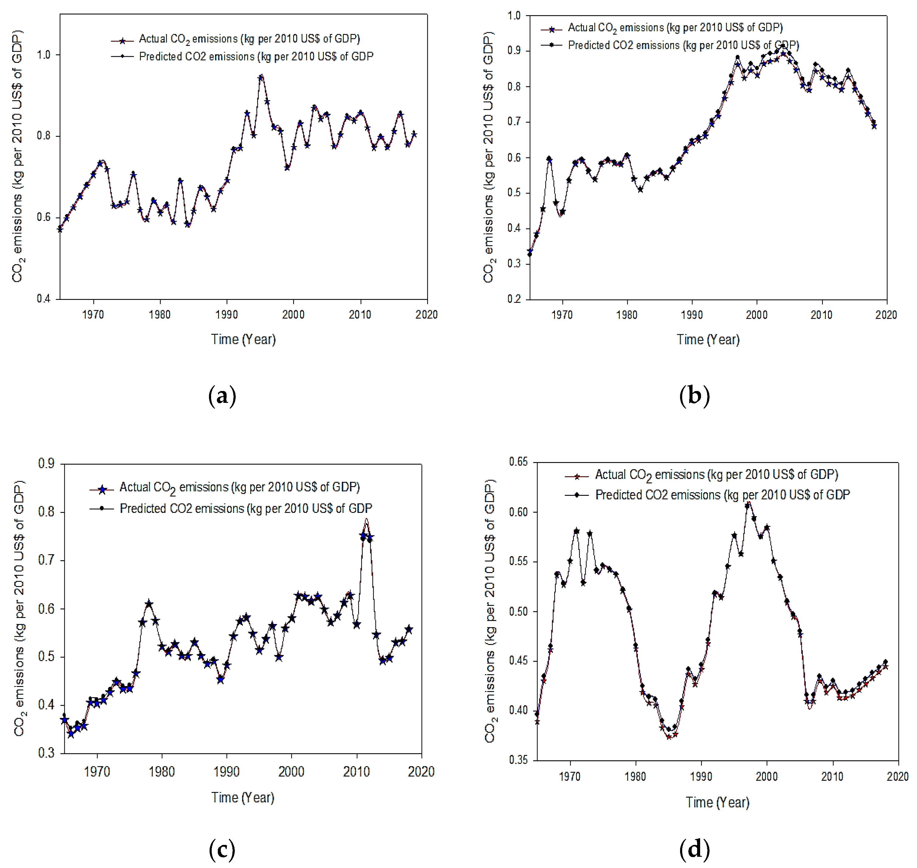
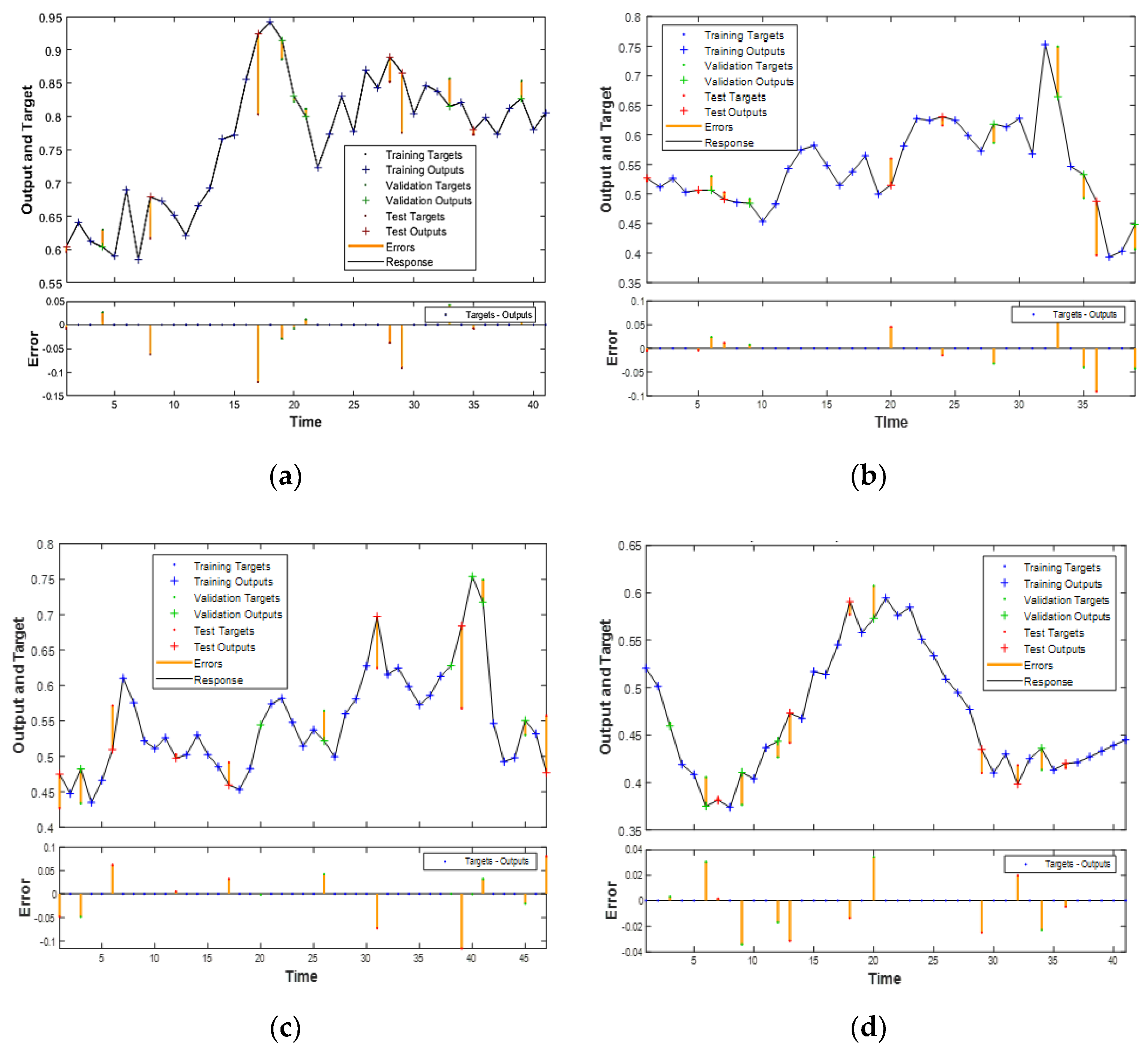
3.2. Performance Evaluation of the Optimized NARX Model
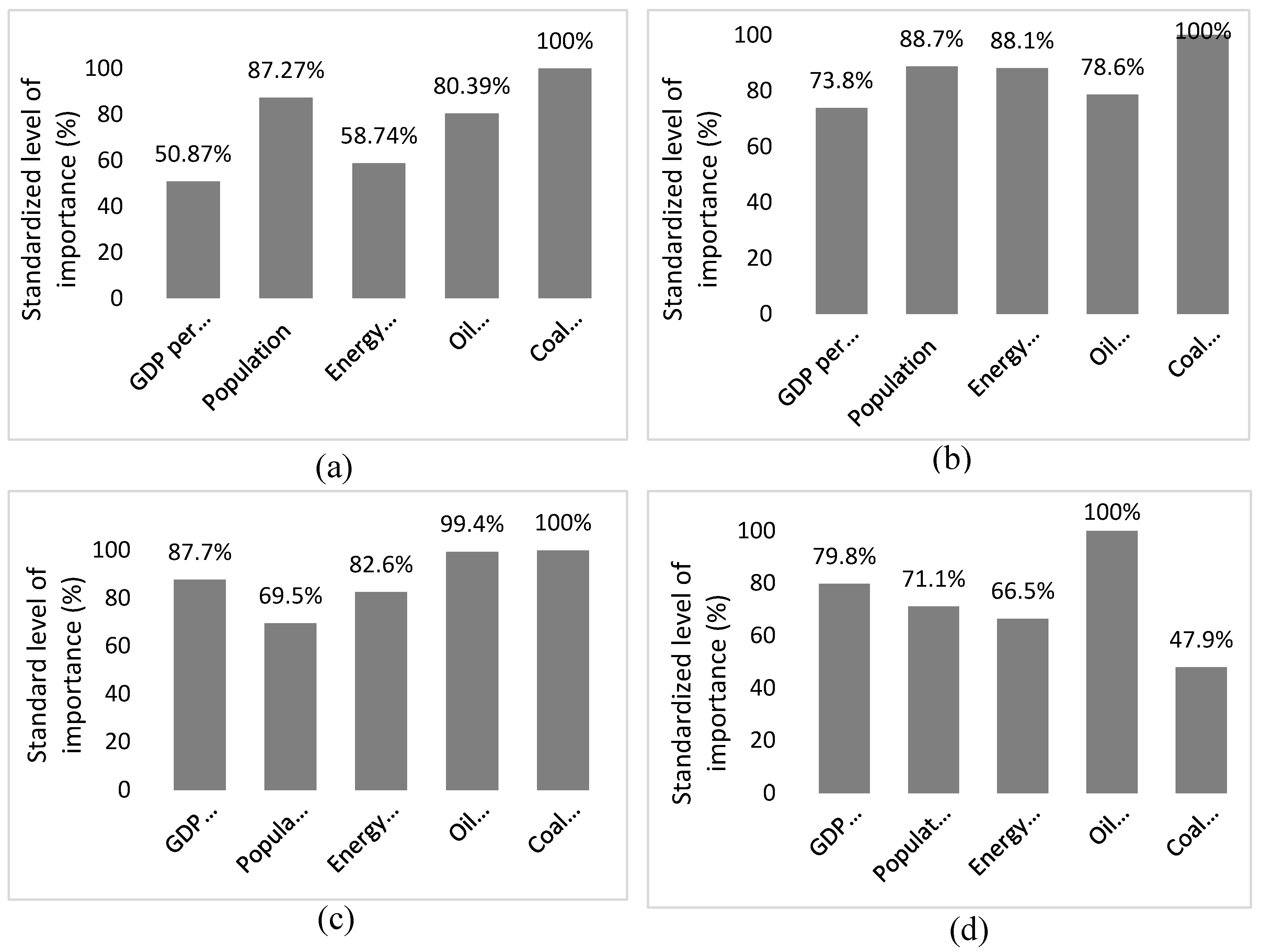
3.3. Sensitivity Analysis to Determine the Level of Importance of the Input Variables
4. Conclusions and Policy Implications
Author Contributions
Funding
Acknowledgments
Conflicts of Interest
Abbreviations
| ASEAN | Association of Southeast Asian Nations |
| ARIMA | Auto-Regressive Integrated Moving Average |
| ARDL | Autoregressive Distributive Lag |
| CO2 | Carbon dioxide |
| EKC | Environmental Kuznets Curve |
| FDI | Foreign Direct Investment |
| MSE | Mean Square Error |
| NARX | Non-linear Autoregressive neural network with Exogenous input |
| MAPE | Mean Absolute Percentage Error |
| TOE | Tonne of Oil Equivalent |
Appendix A

| Number of Delay | 1 | 3 | 5 | 7 | 9 | 11 | 13 | 15 | ||||||||
|---|---|---|---|---|---|---|---|---|---|---|---|---|---|---|---|---|
| Hidden Neurons | MSE | R | MSE | R | MSE | R | MSE | R | MSE | R | MSE | R | MSE | R | MSE | R |
| 1 | 2.54 × 10⁻³ | 0.871 | 1.56 × 10⁻³ | 0.907 | 1.85 × 10⁻³ | 0.899 | 2.32 × 10⁻³ | 0.882 | 3.24 × 10⁻³ | 0.813 | 2.80 × 10⁻³ | 0.844 | 1.77 × 10⁻³ | 0.818 | 3.42 × 10⁻³ | 0.892 |
| 3 | 2.13 × 10⁻³ | 0.892 | 9.46 × 10⁻⁴ | 0.939 | 2.01 × 10⁻³ | 0.900 | 5.75 × 10⁻³ | 0.641 | 3.84 × 0−3 | 0.791 | 1.74 × 10⁻³ | 0.912 | 4.24 × 10⁻⁴ | 0.979 | 1.35 × 10⁻³ | 0.936 |
| 5 | 1.78 × 10⁻³ | 0.914 | 2.47 × 10⁻⁴ | 0.875 | 1.24 × 10⁻³ | 0.921 | 3.68 × 10⁻⁴ | 0.978 | 5.72 × 10⁻³ | 0.905 | 1.42 × 10⁻³ | 0.942 | 5.07 × 10⁻³ | 0.878 | 1.21 × 10⁻² | 0.516 |
| 7 | 1.80 × 10⁻³ | 0.896 | 2.88 × 10⁻³ | 0.881 | 1.43 × 10⁻³ | 0.917 | 1.43 × 10⁻³ | 0.953 | 1.42 × 10⁻⁴ | 0.994 | 2.15 × 10⁻²⁰ | 1.00 | 2.58 × 10⁻³ | 0.941 | 8.34 × 10⁻¹⁷ | 0.999 |
| 9 | 2.07 × 10⁻³ | 0.909 | 4.59 × 10⁻³ | 0.810 | 1.14 × 10⁻³ | 0.924 | 1.28 × 10⁻⁵ | 0.999 | 2.66 × 10⁻³ | 0.989 | 1.43 × 10⁻³ | 0.964 | 9.05 × 10⁻⁴ | 0.958 | 4.08 × 10⁻³ | 0.897 |
| 11 | 1.68 × 10⁻³ | 0.912 | 1.08 × 10⁻³ | 0.932 | 1.24 × 10⁻³ | 0.928 | 8.17 × 10⁻⁴ | 0.961 | 1.46 × 10⁻³ | 0.964 | 2.78 × 10⁻⁵ | 0.998 | 1.06 × 10⁻⁴ | 0.995 | 7.46 × 10⁻⁵ | 0.996 |
| 13 | 1.17 × 10⁻³ | 0.931 | 1.55 × 10⁻³ | 0.901 | 1.74 × 10⁻⁴ | 0.991 | 1.83 × 10⁻⁴ | 0.92 | 6.57 × 10⁻⁵ | 0.998 | 4.13 × 10⁻⁴ | 0.979 | 2.79 × 10⁻³ | 0.9334 | 2.05 × 10⁻⁹ | 0.999 |
| 15 | 1.75 × 10⁻³ | 0.892 | 1.22 × 10⁻³ | 0.933 | 1.05 × 10⁻³ | 0.958 | 8.39 × 10⁻⁴ | 0.974 | 4.16 × 10⁻⁵ | 0.998 | 8.37 × 10⁻³ | 0.702 | 2.51 × 10⁻⁴ | 0.997 | 2.08 × 10⁻³ | 0.949 |
| 17 | 5.59 × 10⁻⁴ | 0.964 | 2.47 × 10⁻³ | 0.986 | 2.03 × 10⁻⁴ | 0.989 | 1.63 × 10⁻⁴ | 0.952 | 1.32 × 10⁻³ | 0.937 | 3.16 × 10⁻⁵ | 0.998 | 1.32 × 10⁻⁴ | 0.998 | 3.71 × 10⁻⁵ | 0.999 |
| 19 | 1.08 × 10⁻³ | 0.936 | 4.36 × 10⁻³ | 0.976 | 1.22 × 10⁻³ | 0.946 | 6.96 × 10⁻⁴ | 0.96 | 8.69 × 10⁻³ | 0.963 | 4.20 × 10⁻²⁰ | 1.00 | 8.27 × 10⁻⁵ | 0.997 | 1.32 × 10⁻³ | 0.974 |
| 21 | 1.65 | 0.898 | 1.10 × 10⁻³ | 0.945 | 3.46 × 10⁻⁴ | 0.989 | 1.45 × 10⁻³ | 0.931 | 1.55 × 10⁻³ | 0.992 | 2.54 × 10⁻³ | 0.883 | 8.38 × 10⁻⁹ | 0.999 | 4.24 × 10⁻⁴ | 0.977 |
| 23 | 2.38 × 10⁻³ | 0.887 | 7.88 × 10⁻⁴ | 0.957 | 8.78 × 10⁻⁴ | 0.975 | 3.25 × 10⁻³ | 0.983 | 3.15 × 10⁻⁴ | 0.988 | 3.37 × 10⁻¹⁷ | 0.999 | 3.25 × 10⁻¹⁶ | 0.999 | 7.37 × 10⁻⁴ | 0.986 |
| 25 | 4.54 × 10⁻⁴ | 0.974 | 1.24 × 10⁻³ | 0.903 | 3.28 × 10⁻³ | 0.885 | 7.19 × 10⁻⁴ | 0.969 | 1.17 × 10⁻³ | 0.978 | 2.99 × 10⁻⁴ | 0.987 | 4.41 × 10⁻⁹ | 0.999 | 5.86 × 10⁻⁴ | 0.977 |
| 27 | 9.17 × 10⁻⁴ | 0.957 | 8.12 × 10⁻⁵ | 0.996 | 8.48 × 10⁻⁴ | 0.953 | 2.35 × 10⁻⁴ | 0.994 | 1.03 × 10⁻⁴ | 0.995 | 1.11 × 10⁻⁴ | 0.986 | 3.63 × 10⁻⁴ | 0.984 | 1.61 × 10⁻² | 0.699 |
| 29 | 1.37 × 10⁻³ | 0.925 | 8.71 × 10⁻³ | 0.965 | 1.15 × 10⁻⁴ | 0.998 | 4.28 × 10⁻³ | 0.924 | 4.84 × 10⁻³ | 0.915 | 2.09 × 10⁻⁸ | 0.999 | 3.92 × 10⁻²¹ | 0.999 | 2.16 × 10⁻⁴ | 0.998 |
| Number of Delays | 1 | 3 | 5 | 7 | 9 | 11 | 13 | 15 | ||||||||
|---|---|---|---|---|---|---|---|---|---|---|---|---|---|---|---|---|
| Hidden Neuron | MSE | R | MSE | R | MSE | R | MSE | R | MSE | R | MSE | R | MSE | R | MSE | R |
| 1 | 2.3 × 10⁻³ | 0.381 | 7.07 × 10⁻⁴ | 0.933 | 7.37 × 10⁻⁴ | 0.944 | 8.96 × 10⁻³ | 0.548 | 7.69 × 10⁻³ | 0.117 | 1.44 × 10⁻³ | 0.898 | 1.12 × 10⁻³ | 0.967 | 2.4 × 10⁻³ | 0.805 |
| 3 | 1.31 × 10⁻³ | 0.912 | 5.52 × 10⁻³ | 0.567 | 2.49 × 10⁻³ | 0.806 | 2.23 × 10⁻³ | 0.827 | 2.77 × 10⁻³ | 0.741 | 1.56 | 0.905 | 3.69 × 10⁻⁴ | 0.997 | 8.2 × 10⁻⁴ | 0.957 |
| 5 | 1.101 | 0.937 | 8.00 × 10⁻³ | 0.613 | 1.93 × 10⁻³ | 0.869 | 1.30 × 10⁻³ | 0.900 | 2.55 × 10⁻⁵ | 0.998 | 2.85 × 10⁻³ | 0.786 | 1.44 × 10⁻⁴ | 0.99 | 9.2 × 10⁻¹⁹ | 0.999 |
| 7 | 8.14 × 10⁻⁴ | 0.953 | 9.76 × 10⁻⁴ | 0.948 | 1.5 × 10⁻³ | 0.899 | 1.14 × 10− | 0.931 | 1.21 × 10⁻⁵ | 0.999 | 7.27 × 10⁻⁴ | 0.936 | 4.06 × 10⁻³ | 0.995 | 8.8 × 10⁻¹² | 0.999 |
| 9 | 2.37 × 10⁻³ | 0.863 | 4.19 × 10⁻³ | 0.973 | 1.65 × 10⁻³ | 0.851 | 1.59 × 10⁻³ | 0.875 | 1.77 × 10⁻³ | 0.804 | 8.56 × 10⁻⁵ | 0.997 | 7.53 × 10⁻⁴ | 0.958 | 6.2 × 10⁻⁸ | 0.999 |
| 11 | 3.64 × 10⁻⁴ | 0.979 | 1.48 × 10⁻³ | 0.898 | 1.86 × 10⁻⁷ | 0.999 | 1.51 × 10⁻⁸ | 0.999 | 9.25 × 10⁻⁵ | 0.994 | 1.87 × 10⁻³ | 0.923 | 4.19 × 10⁻³ | 0.772 | 5.9 × 10⁻⁵ | 0.997 |
| 13 | 7.88 × 10⁻³ | 0.627 | 1.04 × 10⁻⁴ | 0.992 | 5.19 × 10⁻⁴ | 0.966 | 5.02 × 10⁻⁴ | 0.947 | 1.81 × 10⁻³ | 0.909 | 5.88 × 10⁻⁴ | 0.964 | 7.93 × 10⁻⁹ | 0.999 | 4.7 × 10⁻³ | 0.813 |
| 15 | 1.88 × 10⁻³ | 0.892 | 1.71 × 10⁻³ | 0.881 | 4.86 × 10⁻³ | 0.613 | 1.05 × 10⁻³ | 0.968 | 8.54 × 10⁻⁴ | 0.923 | 3.02 × 10⁻³ | 0.998 | 1.14 × 10⁻³ | 0.914 | 2.5 × 10⁻³ | 0.914 |
| 17 | 8.71 × 10⁻³ | 0.951 | 6.62 × 10⁻⁴ | 0.954 | 5.56 × 10⁻⁴ | 0.95 | 3.94 × 10⁻³ | 0.817 | 5.30 × 10⁻⁵ | 0.997 | 1.11 × 10⁻³ | 0.937 | 5.08 × 10⁻⁶ | 0.999 | 6.9 × 10⁻¹⁸ | 0.999 |
| 19 | 5.13 × 10⁻³ | 0.963 | 3.7 × 10⁻¹⁰ | 0.999 | 9.38 × 10⁻⁵ | 0.993 | 2.86 × 10⁻⁴ | 0.984 | 8.52 × 10⁻⁵ | 0.995 | 6.90 × 10⁻⁴ | 0.956 | 4.2 × 10⁻²³ | 0.999 | 1.9 × 10⁻⁵ | 0.879 |
| 21 | 8.86 × 10⁻⁴ | 0.949 | 2.75 × 10⁻⁴ | 0.959 | 3.03 × 10⁻³ | 0.847 | 2.45 × 10⁻⁶ | 0.999 | 4.44 × 10⁻³ | 0.963 | 8.09 × 10⁻⁴ | 0.954 | 5.54 × 10⁻⁵ | 0.997 | 7.9 × 10⁻⁵ | 0.994 |
| 23 | 3.26 × 10⁻³ | 0.984 | 5.54 × 10⁻³ | 0.775 | 6.32 × 10⁻¹⁹ | 0.999 | 1.32 × 10⁻⁴ | 0.998 | 1.52 × 10⁻³ | 0.907 | 4.58 × 10⁻⁸ | 0.999 | 1.21 × 10⁻⁹ | 0.999 | 3.1 × 10⁻⁷ | 0.999 |
| 25 | 2.62 × 10⁻³ | 0.874 | 8.83 × 10⁻⁴ | 0.949 | 7.36 × 10⁻⁴ | 0.945 | 4.36 × 10⁻⁴ | 0.971 | 7.21 × 10⁻⁶ | 0.999 | 6.86 × 10⁻²¹ | 0.999 | 8.92 × 10⁻⁴ | 0.931 | 9.5 × 10⁻⁵ | 0.992 |
| 27 | 2.53 × 10⁻³ | 0.856 | 2.81 × 10⁻³ | 0.841 | 4.28 × 10⁻¹³ | 0.999 | 1.52 × 10⁻⁴ | 0.993 | 1.11 × 10⁻⁵ | 0.999 | 6.12 × 10⁻¹¹ | 0.999 | 1.08 × 10⁻⁴ | 0.996 | 1.7 × 10⁻³ | 0.994 |
| 29 | 1.98 × 10⁻⁴ | 0.987 | 7.06 × 10⁻⁴ | 0.974 | 6.58 × 10⁻³ | 0.546 | 2.45 × 10⁻⁵ | 0.998 | 1.84 × 10⁻⁴ | 0.992 | 9.78 × 10⁻⁴ | 0.999 | 2.72 × 10⁻⁵ | 0.999 | 2.4 × 10⁻³ | 0.999 |
| Delay | 1 | 3 | 5 | 7 | 9 | 11 | 13 | 15 | ||||||||
|---|---|---|---|---|---|---|---|---|---|---|---|---|---|---|---|---|
| Hidden Neuron | MSE | R | MSE | R | MSE | R | MSE | R | MSE | R | MSE | R | MSE | R | MSE | R |
| 1 | 2.71 × 10⁻³ | 0.852 | 2.75 × 10⁻³ | 0.811 | 6.84 × 10⁻⁴ | 0.946 | 1.47 × 10⁻³ | 0.837 | 2.14 × 10⁻³ | 0.753 | 6.96 × 10⁻⁵ | 0.993 | 2.14 × 10⁻³ | 0.697 | 1.25 × 10⁻³ | 0.932 |
| 3 | 9.91 × 10⁻⁴ | 0.935 | 8.39 × 10⁻⁴ | 0.885 | 5.21 × 10⁻⁴ | 0.935 | 8.73 × 10⁻⁴ | 0.929 | 3.44 × 10⁻⁴ | 0.952 | 7.33 × 10⁻⁴ | 0.882 | 1.82 × 10⁻³ | 0.865 | 8.37 × 10⁻⁴ | 0.904 |
| 5 | 2.17 × 10⁻³ | 0.855 | 4.34 × 10⁻⁴ | 0.965 | 1.74 × 10⁻³ | 0.832 | 2.85 × 10⁻³ | 0.869 | 1.18 × 10⁻³ | 0.911 | 3.98 × 10⁻³ | 0.684 | 6.76 × 10⁻³ | 0.991 | 5.15 × 10⁻⁴ | 0.939 |
| 7 | 1.52 × 10⁻³ | 0.909 | 1.71 × 10⁻⁴ | 0.99 | 1.12 × 10⁻³ | 0.923 | 3.44 × 10⁻³ | 0.563 | 1.28 × 10⁻³ | 0.984 | 2.59 × 10⁻³ | 0.981 | 1.17 × 10⁻³ | 0.898 | 4.89 × 10⁻³ | 0.739 |
| 9 | 2.07 × 10⁻³ | 0.868 | 1.54 × 10⁻³ | 0.857 | 5.68 × 10⁻⁵ | 0.996 | 3.46 × 10⁻³ | 0.815 | 1.19 × 10⁻⁵ | 0.999 | 4.81 × 10⁻³ | 0.419 | 9.86 × 10⁻⁴ | 0.901 | 2.54 × 10⁻⁴ | 0.972 |
| 11 | 1.44 × 10⁻³ | 0.901 | 8.28 × 10⁻⁵ | 0.992 | 2.09 × 10⁻³ | 0.991 | 9.12 × 10⁻³ | 0.991 | 8.07 × 10⁻⁵ | 0.991 | 9.27 × 10⁻⁶ | 0.995 | 7.8 × 10⁻¹⁰ | 0.999 | 6.69 × 10⁻³ | 0.959 |
| 13 | 1.50 × 10⁻³ | 0.919 | 3.23 × 10⁻⁴ | 0.962 | 1.08 × 10⁻³ | 0.9326 | 1.16 × 10⁻³ | 0.931 | 1.41 × 10⁻³ | 0.831 | 8.68 × 10⁻⁴ | 0.86 | 1.82 × 10⁻⁴ | 0.965 | 4.73 × 10⁻⁵ | 0.998 |
| 15 | 5.54 × 10⁻⁴ | 0.951 | 1.39 × 10⁻⁴ | 0.989 | 6.39 × 10⁻⁶ | 0.999 | 2.01 × 10⁻³ | 0.891 | 7.08 × 10⁻⁵ | 0.993 | 5.01 × 10⁻³ | 0.97 | 2.54 × 10⁻³ | 0.902 | 7.45 × 10⁻³ | 0.995 |
| 17 | 4.51 × 10⁻³ | 0.571 | 1.04 × 10⁻³ | 0.911 | 1.86 × 10⁻⁴ | 0.986 | 2.09 × 10⁻⁶ | 0.999 | 1.38 × 10⁻³ | 0.922 | 1.35 × 10⁻³ | 0.804 | 8.04 × 10⁻⁷ | 0.999 | 9.28 × 10⁻⁵ | 0.994 |
| 19 | 4.63 × 10⁻³ | 0.847 | 2.70 × 10⁻⁴ | 0.985 | 1.83 × 10⁻³ | 0.945 | 1.19 × 10⁻³ | 0.89 | 1.36 × 10⁻¹³ | 0.999 | 4.65 × 10⁻³ | 0.407 | 6.11 × 10⁻⁴ | 0.953 | 1.4 × 10⁻¹³ | 0.999 |
| 21 | 2.13 × 10⁻³ | 0.812 | 7.18 × 10⁻⁶ | 0.999 | 1.23 × 10⁻⁴ | 0.991 | 1.31 × 10⁻³ | 0.864 | 2.87 × 10⁻⁴ | 0.963 | 2.17 × 10⁻³ | 0.734 | 1.94 × 10⁻³ | 0.867 | 1.29 × 10⁻⁴ | 0.996 |
| 23 | 1.12 × 10⁻³ | 0.938 | 7.83 × 10⁻⁴ | 0.947 | 4.01 × 10⁻⁴ | 0.9728 | 1.98 × 10⁻³ | 0.981 | 1.06 × 10⁻³ | 0.819 | 1.8 × 10⁻¹¹ | 0.999 | 5.14 × 10⁻⁴ | 0.929 | 9.79 × 10⁻⁵ | 0.987 |
| 25 | 5.94 | 0.957 | 6.06 × 10⁻⁴ | 0.956 | 8.70 × 10⁻⁴ | 0.992 | 3.03 × 10⁻³ | 0.97 | 3.35 × 10⁻³ | 0.997 | 3.86 × 10⁻⁴ | 0.969 | 5.35 × 10⁻⁸ | 0.999 | 1.75 × 10⁻³ | 0.928 |
| 27 | 1.75 × 10⁻³ | 0.874 | 6.69 × 10⁻⁴ | 0.952 | 1.57 × 10⁻³ | 0.857 | 1.83 × 10⁻³ | 0.986 | 1.41 × 10⁻³ | 0.847 | 2.46 × 10⁻³ | 0.829 | 2.32 × 10⁻³ | 0.759 | 2.12 × 10⁻⁶ | 0.999 |
| 29 | 4.37 × 10⁻⁴ | 0.984 | 2.05 × 10⁻⁴ | 0.986 | 1.75 × 10⁻¹⁷ | 0.999 | 1.25 × 10⁻²¹ | 0.999 | 5.82 × 10⁻⁴ | 0.954 | 3.05 × 10⁻³ | 0.967 | 3.02 × 10⁻³ | 0.992 | 2.0 × 10⁻¹⁹ | 0.999 |
| Delay | 1 | 3 | 5 | 7 | 9 | 11 | 13 | 15 | ||||||||
|---|---|---|---|---|---|---|---|---|---|---|---|---|---|---|---|---|
| Hidden Neuron | MSE | R | MSE | R | MSE | R | MSE | R | MSE | R | MSE | R | MSE | R | MSE | R |
| 1 | 3.55 × 10⁻⁴ | 0.955 | 4.27 × 10⁻⁴ | 0.955 | 2.12 × 10⁻³ | 0.978 | 4.06 × 10⁻³ | 0.966 | 1.14 × 10⁻⁶ | 0.999 | 8.8 × 10⁻⁵ | 0.992 | 1.21 × 10⁻⁴ | 0.985 | 9.64 × 10⁻⁵ | 0.989 |
| 3 | 3.73 × 10⁻⁴ | 0.96 | 6.95 × 10⁻⁴ | 0.937 | 2.08 × 10⁻³ | 0.981 | 6.64 × 10⁻³ | 0.937 | 6.92 × 10⁻⁵ | 0.992 | 2.35 × 10⁻⁴ | 0.973 | 1.05 × 10⁻⁴ | 0.995 | 2.11 × 10⁻³ | 0.976 |
| 5 | 3.13 × 10⁻⁴ | 0.967 | 2.32 × 10⁻⁴ | 0.973 | 1.13 × 10⁻³ | 0.904 | 2.56 × 10⁻⁴ | 0.907 | 5.61 × 10⁻⁵ | 0.994 | 6.12 × 10⁻⁴ | 0.992 | 1.41 × 10⁻¹⁹ | 0.999 | 5.59 × 10⁻⁵ | 0.995 |
| 7 | 8.76 × 10⁻⁴ | 0.914 | 3.41 × 10⁻⁴ | 0.969 | 1.64 × 10⁻⁴ | 0.987 | 2.71 × 10⁻⁴ | 0.973 | 1.94 × 10⁻⁴ | 0.979 | 7.09 × 10⁻⁵ | 0.994 | 4.08 × 10⁻¹¹ | 0.999 | 3.88 × 10⁻⁵ | 0.996 |
| 9 | 2.61 × 10⁻⁴ | 0.973 | 2.40 × 10⁻⁸ | 0.999 | 1.45 × 10⁻³ | 0.906 | 7.52 × 10⁻⁵ | 0.993 | 9.48 × 10⁻⁵ | 0.993 | 4.98 × 10⁻⁴ | 0.957 | 4.56 × 10⁻⁶ | 0.999 | 5.95 × 10⁻⁵ | 0.994 |
| 11 | 4.24 × 10⁻⁴ | 0.948 | 2.16 × 10⁻⁴ | 0.977 | 2.56 × 10⁻⁴ | 0.981 | 2.9 × 10⁻¹³ | 0.999 | 2.04 × 10⁻⁴ | 0.983 | 6.07 × 10⁻⁵ | 0.995 | 1.21 × 10⁻⁴ | 0.992 | 5.51 × 10⁻⁴ | 0.969 |
| 13 | 1.18 × 10⁻⁴ | 0.979 | 7.92 × 10⁻⁵ | 0.991 | 1.95 × 10⁻⁵ | 0.998 | 2.14 × 10⁻⁵ | 0.998 | 7.89 × 10⁻⁵ | 0.993 | 8.48 × 10⁻⁵ | 0.992 | 2.46 × 10⁻⁴ | 0.978 | 1.32 × 10⁻²⁰ | 0.999 |
| 15 | 1.14 × 10⁻³ | 0.827 | 2.48 × 10⁻⁵ | 0.997 | 3.31 × 10⁻⁴ | 0.975 | 1.73 × 10⁻⁴ | 0.985 | 4.36 × 10⁻⁵ | 0.995 | 2.27 × 10⁻⁵ | 0.998 | 3.66 × 10⁻⁵ | 0.996 | 9.91 × 10⁻⁸ | 0.999 |
| 17 | 3.17 × 10⁻⁴ | 0.966 | 9.55 × 10⁻⁴ | 0.989 | 4.99 × 10⁻⁶ | 0.999 | 8.8 × 10⁻¹⁰ | 0.999 | 4.86 × 10⁻⁵ | 0.996 | 6.65 × 10⁻⁵ | 0.994 | 4.32 × 10⁻⁵ | 0.997 | 1.21 × 10⁻⁵ | 0.999 |
| 19 | 8.43 × 10⁻⁵ | 0.989 | 5.94 × 10⁻⁵ | 0.993 | 4.56 × 10⁻⁵ | 0.996 | 7.15 × 10⁻⁴ | 0.936 | 4.18 × 10⁻¹⁰ | 0.999 | 6.22 × 10⁻⁹ | 0.999 | 2.82 × 10⁻⁵ | 0.998 | 2.22 × 10⁻⁴ | 0.979 |
| 21 | 3.59 × 10⁻⁴ | 0.966 | 2.09 × 10⁻⁴ | 0.981 | 3.56 × 10⁻⁴ | 0.974 | 1.64 × 10⁻³ | 0.908 | 1.09 × 10⁻⁶ | 0.999 | 2.11 × 10¹⁷ | 0.999 | 3.42 × 10⁻⁵ | 0.996 | 1.49 × 10⁻⁸ | 0.999 |
| 23 | 7.05 × 10⁻⁴ | 0.992 | 1.47 × 10⁻⁴ | 0.983 | 1.81 × 10⁻⁴ | 0.982 | 1.45 × 10⁻³ | 0.901 | 1.62 × 10⁻⁴ | 0.987 | 6.85 × 10⁻⁵ | 0.993 | 8.38 × 10⁻⁶ | 0.999 | 5.22 × 10⁻⁴ | 0.972 |
| 25 | 2.38 × 10⁻⁴ | 0.971 | 1.76 × 10⁻⁵ | 0.998 | 5.59 × 10⁻⁴ | 0.931 | 7.29 × 10⁻⁵ | 0.995 | 6.97 × 10⁻¹⁹ | 0.999 | 2.23 × 10⁻⁵ | 0.998 | 3.45 × 10⁻⁴ | 0.959 | 2.89 × 10⁻⁵ | 0.998 |
| 27 | 5.80 × 10⁻⁴ | 0.929 | 4.94 × 10⁻⁵ | 0.994 | 1.26 × 10⁻⁴ | 0.987 | 7.90 × 10⁻⁵ | 0.993 | 2.61 × 10−−5 | 0.997 | 4.36 × 10¹⁷ | 0.999 | 4.91 × 10⁻¹⁴ | 0.999 | 7.96 × 10⁻⁶ | 0.999 |
| 29 | 1.24 × 10⁻⁴ | 0.988 | 6.29 × 10⁻⁵ | 0.994 | 1.78 × 10⁻⁴ | 0.981 | 2.18 × 10⁻⁴ | 0.976 | 4.88 × 10⁻⁴ | 0.935 | 6.25 × 10⁻⁷ | 0.999 | 8.82 × 10⁻²⁰ | 0.999 | 8.92 × 10⁻⁶ | 0.999 |
References
- Wang, Y.; Chen, L.; Kubota, J. The relationship between urbanization, energy use and carbon emissions: Evidence from a panel of Association of Southeast Asian Nations (ASEAN) countries. J. Clean. Prod. 2016, 112, 1368–1374. [Google Scholar] [CrossRef]
- Tongsopit, S.; Kittner, N.; Chang, Y.; Aksornkij, A.; Wangjiraniran, W. Energy security in ASEAN: A quantitative approach for sustainable energy policy. Energy Policy 2016, 90, 60–72. [Google Scholar] [CrossRef]
- Shi, X. The future of ASEAN energy mix: A SWOT analysis. Renew. Sustain. Energy Rev. 2016, 53, 672–680. [Google Scholar] [CrossRef]
- Silberglitt, R.; Kimmel, S. Energy scenarios for Southeast Asia. Technol. Forecast. Soc. Chang. 2015, 101, 251–262. [Google Scholar] [CrossRef]
- International Energy Agency Southeast Asia Energy Outlook 2017; Southeast Asia Energy Outlook: Paris, France, 2017.
- Mensah, I.A.; Sun, M.; Gao, C.; Omari-Sasu, A.Y.; Zhu, D.; Ampimah, B.C.; Quarcoo, A. Analysis on the nexus of economic growth, fossil fuel energy consumption, CO2 emissions and oil price in Africa based on a PMG panel ARDL approach. J. Clean. Prod. 2019, 228, 161–174. [Google Scholar] [CrossRef]
- Mardani, A.; Štreimikienė, D.; Cavallaro, F.; Loganathan, N.; Khoshnoudi, M. Carbon dioxide (CO2) emissions and economic growth: A systematic review of two decades of research from 1995 to 2017. Sci. Total Environ. 2019, 649, 31–49. [Google Scholar] [CrossRef]
- Kasman, A.; Duman, Y.S. CO2 emissions, economic growth, energy consumption, trade and urbanization in new EU member and candidate countries: A panel data analysis. Econ. Model. 2015, 44, 97–103. [Google Scholar] [CrossRef]
- Tzeremes, P. Time-varying causality between energy consumption, CO2 emissions, and economic growth: Evidence from US states. Envrion. Sci. Pollut. Res. 2017, 25, 6044–6060. [Google Scholar] [CrossRef]
- Ozcan, B.; Tzeremes, P.G.; Tzeremes, N.G. Energy consumption, economic growth and environmental degradation in OECD countries. Econ. Model. 2020, 84, 203–213. [Google Scholar] [CrossRef]
- Zhu, H.; Duan, L.; Guo, Y.; Yu, K. The effects of FDI, economic growth and energy consumption on carbon emissions in ASEAN-5: Evidence from panel quantile regression. Econ. Model. 2016, 58, 237–248. [Google Scholar] [CrossRef] [Green Version]
- Heidari, H.; Katircioğlu, S.T.; Saeidpour, L. Economic growth, CO2 emissions, and energy consumption in the five ASEAN countries. Int. J. Electr. Power Energy Syst. 2015, 64, 785–791. [Google Scholar] [CrossRef]
- Salman, M.; Long, X.; Dauda, L.; Mensah, C.N.; Muhammad, S. Different impacts of export and import on carbon emissions across 7 ASEAN countries: A panel quantile regression approach. Sci. Total Environ. 2019, 686, 1019–1029. [Google Scholar] [CrossRef] [PubMed]
- Nugraha, A.T.; Osman, N.H. CO2 emissions, economic growth, energy consumption, and household expenditure for Indonesia: Evidence from cointegration and vector error correction model. Int. J. Energy Econ. Policy 2019, 9, 291–298. [Google Scholar] [CrossRef]
- Fatima, S.; Ali, S.S.; Zia, S.S.; Hussain, E.; Fraz, T.R.; Khan, M.S. Forecasting Carbon Dioxide Emission of Asian Countries Using ARIMA and Simple Exponential Smoothing Models. Int. J. Econ. Environ. Geol. 2019, 10, 64–69. [Google Scholar] [CrossRef]
- Hanif, I.; Raza, S.M.F.; Gago-De-Santos, P.; Abbas, Q. Fossil fuels, foreign direct investment, and economic growth have triggered CO2 emissions in emerging Asian economies: Some empirical evidence. Energy 2019, 171, 493–501. [Google Scholar] [CrossRef]
- Xu, G.; Schwarz, P.; Yang, H. Determining China’s CO2 emissions peak with a dynamic nonlinear artificial neural network approach and scenario analysis. Energy Policy 2019, 128, 752–762. [Google Scholar] [CrossRef]
- Kahouli, B. The causality link between energy electricity consumption, CO2 emissions, R&D stocks and economic growth in Mediterranean countries (MCs). Energy 2018, 145, 388–399. [Google Scholar] [CrossRef]
- Marcjasz, G.; Uniejewski, B.; Weron, R. On the importance of the long-term seasonal component in day-ahead electricity price forecasting with NARX neural networks. Int. J. Forecast. 2019, 35, 1520–1532. [Google Scholar] [CrossRef]
- Alsaffar, M.A.; Ayodele, B.V.; Mustapa, S.I. Scavenging carbon deposition on alumina supported cobalt catalyst during renewable hydrogen-rich syngas production by methane dry reforming using artificial intelligence modeling technique. J. Clean. Prod. 2020, 247, 119168. [Google Scholar] [CrossRef]
- Yang, Z.; Zhao, Y. Energy consumption, carbon emissions, and economic growth in India: Evidence from directed acyclic graphs. Econ. Model. 2014, 38, 533–540. [Google Scholar] [CrossRef]
- Omri, A.; Nguyen, D.K.; Rault, C. Causal interactions between CO2 emissions, FDI, and economic growth: Evidence from dynamic simultaneous-equation models. Econ. Model. 2014, 42, 382–389. [Google Scholar] [CrossRef] [Green Version]
- Feng, Y.; Chen, S.; Zhang, L. System dynamics modeling for urban energy consumption and CO2 emissions: A case study of Beijing, China. Ecol. Model. 2013, 252, 44–52. [Google Scholar] [CrossRef]
- Pao, H.-T.; Yu, H.-C.; Yang, Y.-H. Modeling the CO2 emissions, energy use, and economic growth in Russia. Energy 2011, 36, 5094–5100. [Google Scholar] [CrossRef]
- Alam, M.J.; Begum, I.A.; Buysse, J.; Rahman, S.; Van Huylenbroeck, G. Dynamic modeling of causal relationship between energy consumption, CO2 emissions and economic growth in India. Renew. Sustain. Energy Rev. 2011, 15, 3243–3251. [Google Scholar] [CrossRef]
- Maziarz, M. A review of the Granger-causality fallacy. J. Philos. Econ. Reflect. Econ. Soc. Issues 2015, 8, 86–105. [Google Scholar]
- Liu, X.; Mao, G.; Ren, J.; Li, R.Y.M.; Guo, J.; Zhang, H.-L. How might China achieve its 2020 emissions target? A scenario analysis of energy consumption and CO2 emissions using the system dynamics model. J. Clean. Prod. 2015, 103, 401–410. [Google Scholar] [CrossRef]
- Govindaraju, V.C.; Tang, C.F. The dynamic links between CO2 emissions, economic growth and coal consumption in China and India. Appl. Energy 2013, 104, 310–318. [Google Scholar] [CrossRef]
- Hossain, M.A.; Ayodele, B.V.; Cheng, C.K.; Khan, M.R. Artificial neural network modeling of hydrogen-rich syngas production from methane dry reforming over novel Ni/CaFe2O4 catalysts. Int. J. Hydrog. Energy 2016, 41, 11119–11130. [Google Scholar] [CrossRef] [Green Version]
- Saghafi, M.; Ghofrani, M.B. Real-time estimation of break sizes during LOCA in nuclear power plants using NARX neural network. Nucl. Eng. Technol. 2019, 51, 702–708. [Google Scholar] [CrossRef]
- Rahmani, A.; Deihimi, A. Reduction of harmonic monitors and estimation of voltage harmonics in distribution networks using wavelet analysis and NARX. Electr. Power Syst. Res. 2020, 178, 106046. [Google Scholar] [CrossRef]
- Ezzeldin, R.; Hatata, A.Y. Application of NARX neural network model for discharge prediction through lateral orifices. Alex. Eng. J. 2018, 57, 2991–2998. [Google Scholar] [CrossRef]
- Garson, G.D. Comparison of Neural Network Analysis of Social Science Data. Soc. Sci. Comput. Rev. 1991, 9, 399–434. [Google Scholar] [CrossRef]
- Cheng, J.; Ji, Z.; Li, M.; Dai, J. Study of a noninvasive blood glucose detection model using the near-infrared light based on SA-NARX. Biomed. Signal Process. Control 2020, 56, 101694. [Google Scholar] [CrossRef]
- Pazikadin, A.R.; Rifai, D.; Ali, K.; Malik, M.Z.; Abdalla, A.N.; Faraj, M.A. Solar irradiance measurement instrumentation and power solar generation forecasting based on Artificial Neural Networks (ANN): A review of five years research trend. Sci. Total Envrion. 2020, 715, 136848. [Google Scholar] [CrossRef]
- Giannopoulos, A.; Aider, J.-L. Prediction of the dynamics of a backward-facing step flow using focused time-delay neural networks and particle image velocimetry data-sets. Int. J. Heat Fluid Flow 2020, 82, 108533. [Google Scholar] [CrossRef]
- Das, S.K.; Basudhar, P.K. Prediction of residual friction angle of clays using artificial neural network. Eng. Geol. 2008, 100, 142–145. [Google Scholar] [CrossRef]
- Zounemat-Kermani, M.; Stephan, D.; Hinkelmann, R. Multivariate NARX neural network in prediction gaseous emissions within the influent chamber of wastewater treatment plants. Atmos. Pollut. Res. 2019, 10, 1812–1822. [Google Scholar] [CrossRef]
- Oko, E.; Wang, M.; Zhang, J. Neural network approach for predicting drum pressure and level in coal-fired subcritical power plant. Fuel 2015, 151, 139–145. [Google Scholar] [CrossRef]
- Alcan, G.; Unel, M.; Aran, V.; Yilmaz, M.; Gurel, C.; Koprubasi, K. Predicting NOx emissions in diesel engines via sigmoid NARX models using a new experiment design for combustion identification. Measurements 2019, 137, 71–81. [Google Scholar] [CrossRef] [Green Version]
- Koschwitz, D.; Frisch, J.; Van Treeck, C. Data-driven heating and cooling load predictions for non-residential buildings based on support vector machine regression and NARX Recurrent Neural Network: A comparative study on district scale. Energy 2018, 165, 134–142. [Google Scholar] [CrossRef]
- Pakzad, P.; Mofarahi, M.; Izadpanah, A.A.; Afkhamipour, M. Experimental data, thermodynamic and neural network modeling of CO2 absorption capacity for 2-amino-2-methyl-1-propanol (AMP) + Methanol (MeOH) + H2O system. J. Nat. Gas Sci. Eng. 2020, 73, 103060. [Google Scholar] [CrossRef]
- Hamzehie, M.; Mazinani, S.; Davardoost, F.; Mokhtare, A.; Najibi, H.; Van Der Bruggen, B.; Darvishmanesh, S. Developing a feed forward multilayer neural network model for prediction of CO2 solubility in blended aqueous amine solutions. J. Nat. Gas Sci. Eng. 2014, 21, 19–25. [Google Scholar] [CrossRef]
- Energy in Malaysia. Toward a World-Class Energy Sector; Suruhanjaya Tenaga: Putrajaya, Malaysia, 2017; Volume 12, pp. 1–45. [Google Scholar]
- Kenney, W. Energy Conservation in the Process Industries; Elsevier: Amsterdam, The Netherlands, 1984; pp. 1–17. [Google Scholar]
- Gross Energy Generation and Purchase; EGAT: Bangkok, Thailand, 2019.
- Handbook of Energy & Economic Statistics of Indonesia 2018; Ministry of Energy and Mineral Resources, Republic of Indonesia: Jakarta, Indonesia, 2018.
- Philippines Power Statistics; Department of Energy: Taguig, Philippines, 2019.
- Al-Mulali, U.; Sab, C.N.B.C. Electricity consumption, CO2 emission, and economic growth in the Middle East. Energy Sources Part B Econ. Plan. Policy 2018, 13, 257–263. [Google Scholar] [CrossRef]
- Chang, C.-C. A multivariate causality test of carbon dioxide emissions, energy consumption and economic growth in China. Appl. Energy 2010, 87, 3533–3537. [Google Scholar] [CrossRef]
- Apergis, N.; Payne, J.E. CO2 emissions, energy usage, and output in Central America. Energy Policy 2009, 37, 3282–3286. [Google Scholar] [CrossRef]
- Apergis, N.; Payne, J.E. The emissions, energy consumption, and growth nexus: Evidence from the commonwealth of independent states. Energy Policy 2010, 38, 650–655. [Google Scholar] [CrossRef]
- Al-Mulali, U.; Fereidouni, H.G.; Lee, J.Y.; Sab, C.N.B.C. Exploring the relationship between urbanization, energy consumption, and CO2 emission in MENA countries. Renew. Sustain. Energy Rev. 2013, 23, 107–112. [Google Scholar] [CrossRef]
- Saboori, B.; Sulaiman, J. Environmental degradation, economic growth and energy consumption: Evidence of the environmental Kuznets curve in Malaysia. Energy Policy 2013, 60, 892–905. [Google Scholar] [CrossRef]


| Countries Investigated | Methods | Variables | Reference |
|---|---|---|---|
| ASEAN (Malaysia, Thailand, Indonesia and the Philippines) | Autoregressive Exogenous Neural Network Modeling | Energy Consumption per capita, Population, GDP per capita | This study |
| ASEAN (Brunei, Indonesia, Malaysia, Philippines, Singapore, Thailand, Vietnam) | Panel quantile regression approach | Export and Import | [13] |
| Indonesia | Cointegration and Vector Error Correction Model | Energy Consumption, GDP, House Expenditure | [14] |
| Asian countries (Japan, Bangladesh, China, Pakistan, India, Sri Lanka, Iran, Singapore, and Nepal) | Auto-Regressive Integrated Moving Average (ARIMA) and Simple Exponential Smoothing Models | Heat and electricity, manufacturing industries, residential and commercial buildings, transport | [15] |
| Asia countries | Autoregressive Distributive Lag model. | Fossil fuel, FDI, GDP | [16] |
| China | Linear regression, Backpropagation neural network, non-linear dynamic neural network | GDP, total population, urbanization rate, total energy consumption, percentage of coal consumption, percentage of non-fossil consumption | [17] |
| Mediterranean countries | System of simultaneous equations using seemingly unrelated regression. | Research and Development Stocks, GDP. Electricity Consumption, | [18] |
| Croatia | Environmental Kuznets Curve (EKC) model | GDP | [18] |
| ASEAN (Malaysia, Indonesia, Philippines, Singapore, and Thailand) | Panel quantile regression model | Foreign Direct Investment, GDP, Energy Consumption | [11] |
| ASEAN (Malaysia, Indonesia, Philippines, Singapore, and Thailand) | Panel smooth transition regression model | Energy Consumption and GDP | [12] |
| India | Directed acyclic graphs | Energy Consumption, GDP, fixed capita formation, and Trade openness | [21] |
| Middle East, North Africa and Sub-Sahara Africa | Simultaneous Equation Models | Foreign direct investment, | [22] |
| China | System Dynamic Modelling | Energy Consumptions | [23] |
| Russia | Environmental Kuznets Curve (EKC) model | Energy Consumptions and GDP | [24] |
| India | System Dynamic Modelling | Energy Consumption and GDP | [25] |
| Turkey | autoregressive distributed lag bounds testing approach of cointegration | Energy consumption and economic indicator | [26] |
| Model Architecture | Delay | Hidden Neurons | R | R2 | MSE |
|---|---|---|---|---|---|
| 5-25-1 | 1 | 25 | 0.974 | 0.949 | 4.54 × 10⁻⁴ |
| 5-27-1 | 3 | 27 | 0.996 | 0.992 | 8.12 × 10⁻⁵ |
| 5-29-1 | 5 | 29 | 0.998 | 0.996 | 1.15 × 10⁻⁴ |
| 5-9-1 | 7 | 9 | 0.999 | 0.998 | 1.28 × 10⁻⁵ |
| 5-15-1 | 9 | 15 | 0.998 | 0.996 | 4.16 × 10⁻⁵ |
| 5-7-1 | 11 | 7 | 0.999 | 0.998 | 2.15 × 10⁻²⁰ |
| 5-29-1 | 13 | 29 | 0.999 | 0.998 | 3.92 × 10⁻²¹ |
| 5-7-1 | 15 | 7 | 0.999 | 0.998 | 8.34 × 10⁻¹⁷ |
| Model Architecture | Delay | Hidden Neurons | R | R2 | MSE |
|---|---|---|---|---|---|
| 5-29-1 | 1 | 29 | 0.987 | 0.974 | 1.98 × 10⁻⁴ |
| 5-19-1 | 3 | 19 | 0.999 | 0.998 | 3.72 × 10⁻¹⁰ |
| 5-23-1 | 5 | 23 | 0.999 | 0.998 | 6.32 × 10⁻¹⁹ |
| 5-11-1 | 7 | 11 | 0.999 | 0.998 | 1.51 × 10⁻⁸ |
| 5-25-1 | 9 | 25 | 0.999 | 0.998 | 7.21 × 10⁻⁶ |
| 5-25-1 | 11 | 25 | 0.999 | 0.998 | 6.86 × 10⁻²¹ |
| 5-19-1 | 13 | 19 | 0.999 | 0.998 | 4.15 × 10⁻²³ |
| 5-5-1 | 15 | 5 | 0.999 | 0.998 | 9.18 × 10⁻¹⁹ |
| Model Architecture | Delay | Hidden Neurons | R | R2 | MSE |
|---|---|---|---|---|---|
| 5-29-1 | 1 | 29 | 0.984 | 0.968 | 4.37 × 10⁻⁴ |
| 5-21-1 | 3 | 21 | 0.999 | 0.998 | 7.18 × 10⁻⁶ |
| 5-29-1 | 5 | 29 | 0.999 | 0.998 | 1.75 × 10⁻¹⁷ |
| 5-29-1 | 7 | 29 | 0.999 | 0.998 | 1.25 × 10⁻²¹ |
| 5-19-1 | 9 | 19 | 0.999 | 0.998 | 1.36 × 10⁻¹³ |
| 5-23-1 | 11 | 23 | 0.999 | 0.998 | 1.83 × 10⁻¹¹ |
| 5-25-1 | 13 | 25 | 0.999 | 0.998 | 5.35 × 10⁻⁸ |
| 5-17-1 | 15 | 17 | 0.999 | 0.998 | 2.02 × 10⁻¹⁹ |
| Model Architecture | Delay | Hidden Neurons | R | R2 | MSE |
|---|---|---|---|---|---|
| 5-23-1 | 1 | 23 | 0.992 | 0.984 | 7.05 × 10⁻⁵ |
| 5-9-1 | 3 | 9 | 0.999 | 0.998 | 2.40 × 10⁻⁸ |
| 5-17-1 | 5 | 17 | 0.999 | 0.998 | 4.99 × 10⁻⁶ |
| 5-11-1 | 7 | 11 | 0.999 | 0.998 | 2.94 × 10⁻¹³ |
| 5-25-1 | 9 | 25 | 0.999 | 0.998 | 6.97 × 10⁻¹⁹ |
| 5-21-1 | 11 | 21 | 0.999 | 0.998 | 2.11 × 10⁻¹⁷ |
| 5-29-1 | 13 | 29 | 0.999 | 0.998 | 8.82 × 10⁻²⁰ |
| 5-13-1 | 15 | 13 | 0.999 | 0.998 | 1.32 × 10⁻²⁰ |
| Malaysia | Thailand | Indonesia | Philippines | |
|---|---|---|---|---|
| Input units | 5 | 5 | 5 | 5 |
| Optimized hidden neurons | 13 | 19 | 17 | 13 |
| Optimized delay | 13 | 13 | 15 | 15 |
| Output units | 1 | 1 | 1 | 1 |
| Reference | Modelling Techniques | Objectives | Input Variables | Measurement of Accuracy | Conclusions |
|---|---|---|---|---|---|
| This work | NARX neural network | Predictive modelling of CO2 emissions in four ASEAN countries | Energy consumption per capita, GDP per capita, population, oil consumption, coal consumption | MSE values of 6.93 × −4, 9.26 × 10⁻⁴, 2.03 × 10⁻³, and 7.99 × 10⁻⁴ obtained for CO2 emissions in Malaysia, Thailand, Indonesia, and the Philippines | The optimized NARX models efficiently predicted CO2 emissions I the four ASEAN countries with coal consumptions having the highest level of importance. |
| Alcan et al. [40] | NARX neural network | Predictive modelling of NOx emissions from diesel engines | Engine speed, Manifold Absolute Pressure, Mass Air Flow, rail pressure, main and pilot injection fuel quantities, Main and pilot start of injections | Not reported | The optimized NARX model architecture predicted the NOx emissions with high degree of accuracy |
| Xu et al. [17] | NARX neural network | Predict CO2 emission in China | GDP, total population, industrialization, urbanization, secondary sector, tertiary sector, total energy consumption, coal consumption, non-fossil consumption, energy productivity, investment in environment governance | RMSE = 0.0311 | Economic scale, secondary sector (manufacturing and construction), coal consumption, industrialization, and energy productivity significantly influenced CO2 emissions |
| Koschwitz et al. [41] | NARX neural network and Support Vector Machine | Prediction of energy consumption in commercial building | dew point temperature, mean wind direction, mean wind velocity, outdoor temperature, precipitation intensity, precipitation quantity, relative humidity, school holiday time, working time schedule | MSE = 2.35–2.89 | NARX models displayed a better prediction of the energy consumption in the non-commercial buildings compared to support vector machine |
| Pakzad et al. [42] | Multilayer Perceptron Neural Network | Modelling the CO2 absorption | CO2 partial pressure, temperature, AMP concentration, and MeOH concentration | Average absolute relative deviation (AARD%) = 1.95 | The findings revealed that the ANN models predicted CO2 absorption was in proximity with the observed. |
| Hamzehie et al. [43] | Multilayer Perceptron Neural Network | Modelling the CO2 solubility | Temperature, pressure, overall concentration, apparent molecular weight of the mixture. | MSE = 2.300 × 10⁻⁴ | The solubility of CO2 in the mixed aqueous solution was accurately predicted by the Neural Network. |
Publisher’s Note: MDPI stays neutral with regard to jurisdictional claims in published maps and institutional affiliations. |
© 2020 by the authors. Licensee MDPI, Basel, Switzerland. This article is an open access article distributed under the terms and conditions of the Creative Commons Attribution (CC BY) license (http://creativecommons.org/licenses/by/4.0/).
Share and Cite
Mustapa, S.I.; Ayodele, F.O.; Ayodele, B.V.; Mohammad, N. Nexus between Energy Usability, Economic Indicators and Environmental Sustainability in Four ASEAN Countries: A Non-Linear Autoregressive Exogenous Neural Network Modelling Approach. Processes 2020, 8, 1529. https://doi.org/10.3390/pr8121529
Mustapa SI, Ayodele FO, Ayodele BV, Mohammad N. Nexus between Energy Usability, Economic Indicators and Environmental Sustainability in Four ASEAN Countries: A Non-Linear Autoregressive Exogenous Neural Network Modelling Approach. Processes. 2020; 8(12):1529. https://doi.org/10.3390/pr8121529
Chicago/Turabian StyleMustapa, Siti Indati, Freida Ozavize Ayodele, Bamidele Victor Ayodele, and Norsyahida Mohammad. 2020. "Nexus between Energy Usability, Economic Indicators and Environmental Sustainability in Four ASEAN Countries: A Non-Linear Autoregressive Exogenous Neural Network Modelling Approach" Processes 8, no. 12: 1529. https://doi.org/10.3390/pr8121529