Review

Revisiting the Role of Mass and Heat Transfer in Gas–Solid Catalytic Reactions

by
Riccardo Tesser
1 and
Elio Santacesaria
2,*
1
NICL—Naples Industrial Chemistry Laboratory, Department of Chemical Science, University of Naples Federico II, 80126 Naples, Italy
2
CEO of Eurochem Engineering Ltd., 20139 Milan, Italy
*
Author to whom correspondence should be addressed.
Processes 2020, 8(12), 1599; https://doi.org/10.3390/pr8121599
Submission received: 14 October 2020 / Revised: 23 November 2020 / Accepted: 2 December 2020 / Published: 4 December 2020

Abstract

:
The tremendous progress in the computing power of modern computers has in the last 20 years favored the use of numerical methods for solving complex problems in the field of chemical kinetics and of reactor simulations considering also the effect of mass and heat transfer. Many classical textbooks dealing with the topic have, therefore, become quite obsolete. The present work is a review of the role that heat and mass transfer have in the kinetic studies of gas–solid catalytic reactions. The scope was to collect in a relatively short document the necessary knowledge for a correct simulation of gas–solid catalytic reactors. The first part of the review deals with the most reliable approach to the description of the heat and mass transfer outside and inside a single catalytic particle. Some different examples of calculations allow for an easier understanding of the described methods. The second part of the review is related to the heat and mass transfer in packed bed reactors, considering the macroscopic gradients that derive from the solution of mass and energy balances on the whole reactor. Moreover, in this second part, some examples of calculations, applied to chemical reactions of industrial interest, are reported for a better understanding of the systems studied.

Graphical Abstract

1. Introduction

When a reaction occurs inside a catalytic particle, the reagents are consumed, giving rise to products and, in the meantime, heat is released or absorbed according to whether the enthalpy of the reaction is positive or negative. Inside and around the particles, gradients of respective concentration and temperature are generated as a consequence. Then, if the particles are put inside a tubular reactor (see Figure 1), macroscopic gradients (both in axial and radial directions) also arise as a consequence of the average rate of reaction in any single catalytic particle and the regime of mass and heat flow developed in the specific reactor. In Figure 1, all the possible gradients related to both temperature and concentration occurring in a tubular gas–solid catalytic reactor are illustrated.
These macroscopic (or “long-range”) gradients can be vanished by employing “gradientless” reactors that are isothermal CSTRs (continuous stirred tank reactors) normally used in laboratory kinetic studies (see Figure 2A,B).
Moreover, each particle inside a reactor has its own history, and microscopic gradients are developed in conditions at the particle surface that are generally different from the internal particle conditions.
At the industrial scale, gas–solid catalytic processes are usually carried out in very large capacity equipment represented by packed bed reactors with productivity of thousands of tons per year.
Such reactors are arranged in a complex scheme also containing all the auxiliary equipment necessary for feeding, cooling, heating, or pressurizing operations. The necessity of supplying or removing heat according to the enthalpy of the reaction is the main reason for which reactors with multiple tubes (in many cases thousands of tubes) are preferred. The heat removal is obtained by circulating an opportune fluid externally to the tubes in order to limit the temperature rise (or drop) of the reactive mixture.
Normally, the goal is to obtain isothermal conditions, however, very frequently, these ideal conditions cannot be reached. On the contrary, when an equilibrium reaction is involved in the reaction scheme, such as for example:
SO 2   +   ½   O 2     SO 3
a single reactor with large diameter, in which structurally different catalytic packed beds are contained and operating in adiabatic conditions, is preferred, because this type of reactor allows for the control of the overall conversion through the temperature of the outlet flow stream. The heat removal, in this case, is obtained by cooling the flow stream between two different catalytic stages of the reactor.
Two ideal limit conditions can be recognized, the isothermal and adiabatic, realized thanks to a more or less efficient system of heat exchange. However, a condition not isothermal and not adiabatic is more frequently encountered in practice. This implies the development of more complex models to describe the system in which the mentioned limit conditions are considered as particular cases.
Some other aspects are important in the design of fixed-bed reactors, such as pressure drop, safe operating protocol (to avoid runaway problems), temperature range, and catalyst packing modality.
From a general point of view, the design approach of catalytic fixed-bed reactors consists in correctly defining and then solving the mass and energy balance equations. Normally, the solution of such equations must be achieved only numerically, especially when the kinetic systems are characterized by a complex reaction scheme. The problem must to be solved simultaneously both at a microscopic local level, with the obtainment of the reagents and product concentration particle profiles, as well as of the effectiveness factor for all the occurring reactions, and at a macroscopic level, reproducing all the long-range concentration and temperature profiles. This specific situation requires an evaluation of the catalyst effectiveness factor in each position in the catalytic bed, considering the conditions we have at any instance in that point. This subject has been previously described in many books, papers, and reviews [1,2,3,4,5,6,7,8,9,10,11,12,13,14,15,16,17]. A modern and comprehensive approach to the problem, with many solved exercises, can be found in [1]. On the basis of all the examined literature, the scope of this review is to give, in a concise way, all the information necessary to the researchers to correctly face the study of the gas–solid reactions. In the following paragraphs, we consider, first of all, the mass and heat transfer occurring in a single catalytic particle, and then we will treat the macroscopic gradients related to the whole fixed-bed reactor.

2. Mass and Heat Transfer in a Single Catalytic Particle

When a reaction occurs inside a catalytic particle, the reagents are consumed for giving products and a certain amount of heat is consumed or released according to the thermal characteristic of the reaction (exothermic or endothermic). The concentration of the reagents decreases from the external geometric surface of the particles toward the center. The concentration of the products, on the contrary, increases. The temperature changes as a consequence of the heat consumed or released by the reaction, increasing or decreasing from the external surface to the center of the catalytic particle. In other words, the reaction is responsible of the concentration and temperature gradients originating inside the particle that act as driving forces for both the mass and heat transfer inside the catalyst particle. The faster the reaction, the steeper the gradients. In the case of high reaction rate, this effect is propagated toward the external part of the catalyst particle, generating other gradients of concentration and temperature between the catalyst surface and the bulk fluid. When the fluid flow regime is turbulent, as normally occurs in industrial reactors, the external gradients are confined to very thin layer, named the boundary layer, that surrounds the solid surface. The boundary layer is quiescent, and consequently mass and heat transfer occur through it, with a relatively slow process characterized by the molecular diffusion mechanism. The effects of reaction and diffusion rates are concentration and temperature profiles, respectively, such as the ones reported in Figure 3. External diffusion and chemical reaction are consecutive steps, and their contributions to the overall reaction rates can be considered separately. A similar approach cannot be adopted for the internal diffusion as it occurs simultaneously with the chemical reaction. To describe the influence of internal diffusion on reaction rate requires solving the mass and heat balance equations related to any single particle for evaluating the concentration and temperature profiles inside the pellet.

2.1. Diffusion with Reaction in a Single Catalytic Particle: Mass and Heat Balance Equations

For a spherical particle, the mass balance can be written by considering the inlet, outlet, reaction, and accumulation terms related to a spherical shell of thickness dr and radius r (see Figure 4):
[ diffusion rate inward at x = x + dx ] - [ diffusion rate outward at x = x ] - [ reaction rate into the shell ] = [ accumulation ]
Assuming steady state conditions, it results null the accumulation term and then
4 π ( x + d x ) 2 N x + d x 4 π x 2 N x 4 π x 2 d x · v r = 0
By introducing the Fick’s law N = D e f f d c d x for the internal diffusive flux and a generic power law for the reaction rate v = SvkScn, related to a single reaction, and through rearranging we obtain
D e f f x 2 d d x ( x 2 d c d x ) S v k S c n = 0
with the boundary conditions
for   x   =   r P   c   =   c S for   x   =   0     d c d x = 0
For the heat balance, it is possible to follow a similar approach by introducing Fourier’s law q = k e f f d T d x instead of Fick’s law, obtaining the following equation:
k e f f x 2 d d x ( x 2 d T d x ) ( Δ H ) S V k S c n = 0
with boundary conditions
for   x = r P     T = T S for   x = 0 d T d x = 0
Considering the common terms of Equations (3) and (4), it is possible to write
( T T S ) = D e f f k e f f ( c c S ) ( Δ H )
From this equation, we can conclude that for any concentration profile, inside the particle, a corresponding profile of temperature can easily be determined by using Equation (5). Alternatively, a full energy balance on the particle must be solved. A maximum temperature gradient ΔTmax can be obtained when the concentration at the center of the particle can be assumed near to zero; in this case, ΔccS, and hence
Δ T max = D e f f k e f f c S ( Δ H )
Referring ΔTmax to TS, the temperature at the catalyst surface, the Prater’s number is obtained, defined as β = Δ T max / T S .
As the thermal conductivity of solid catalyst particles is normally much higher than those of the gaseous reaction mixture, in steady state conditions, internal temperature gradients are rarely important in practice.
The evaluation of the internal profiles of both concentration and temperature requires the solution of Equations (3) and (4). For this purpose, it is opportune to introduce some dimensionless terms such as
ε d r = x / r P γ d r = c / c S ψ d r = v r ( c ) / v r ( c S ) ϕ = r P S V k S c S n 1 D e f f
and Equation (3) for mass conservation becomes
1 ε d r 2 d d ε d r ( ε d r 2 d γ d r d ε d r ) = ϕ 2 ψ d r
where ϕ is called Thiele modulus [18]. It is interesting to observe that for n = 1, the Thiele modulus is independent of the concentration, and consequently Equation (3) or (8) can be solved analitically, while for different reaction orders or complex kinetics, an iterative numerical solution strategy must be adopted.

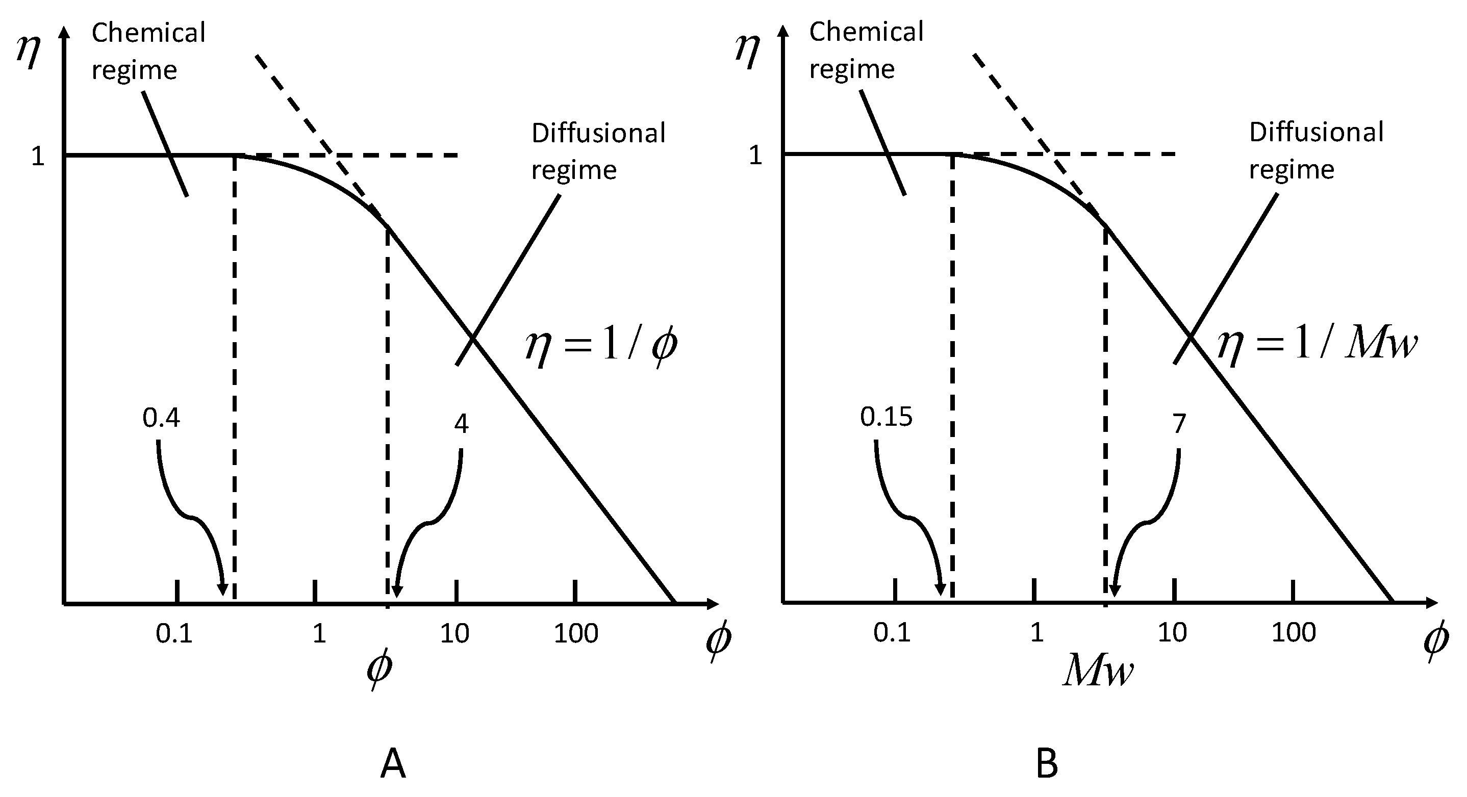
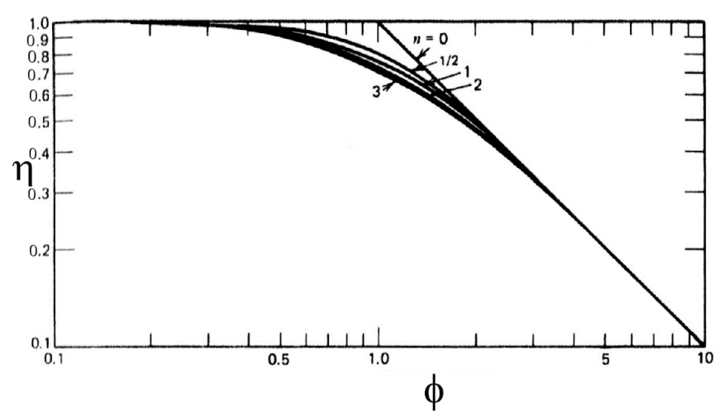
2.2. Definition and Evolution of the Effectiveness Factor

If the internal concentration profile of γ (dimensionless concentration) is known, it is possible to evaluate another dimensionless term η, named “effectiveness factor”, defined as the ratio between the observed reaction rate, more or less affected by the internal diffusion, and the rate occurring in chemical regime, that is, not limited by internal diffusion. We can write
η = effective   reaction   rate reaction   rate   from   kinetic   law
and can write accordingly
η = 0 r p 4 π x 2 v r ( c ) d x 4 3 π r P 3 v r ( c S ) = 3 0 1 ε d r 2 ψ d r ( γ d r ) d ε d r
Therefore, η is a dimensionless factor directly giving the effect of the internal diffusion on the reaction rate. For a reaction rate of a single reaction of n-th order, affected by internal diffusion, we can simply write
v r = η k S S V c S n = η k V c S n
The effectiveness factor η can also be determined by considering that, in steady state conditions, the overall reaction rate in a particle is equal to the rate of external mass transfer from bulk to the surface. Equation (10) can be rewritten as
η = 4 π r P 2 D e f f ( d c d x ) r P 4 3 π r P 3 v r ( c S ) = 3 D e f f ( d c d x ) r P r P k S c S
As mentioned, for reaction order n = 1, the concentration profile can be analytically determined, and this can be done with Equation (13).
d c d x = c S x [ ϕ tanh ϕ 1 ϕ ]
from which the following expression for the effectiveness factor can be derived by assuming a particle with spherical geometry:
η = 3 ϕ [ 1 tanh ϕ 1 ϕ ]
This equation changes with the shape of the catalyst particles, and the Thiele modulus ϕ changes too, as the quantity rP in Equation (7) becomes a characteristic length given by the ratio between volume and external surface area of the catalytic pellet.
In some cases, the kinetic law is unknown, even if the data of the reaction rate are available. The evaluation of the Thiele modulus and of the effectiveness factor in these cases is not possible. For this purpose, it is useful to define another dimensionless modulus, named the “Weisz modulus” [19], through the following relation:
M W = r P 2 v r c S D e f f = ϕ 2 η
The Weisz modulus allows for the evaluation of the effectiveness factor when experimental data of reaction rate are available.
Different plots of η, the “effectiveness factor”, as a function of ϕ or MW can be drawn. Examples of these plots for spherical particles and first-order reactions are reported in Figure 5A,B. In these plots, we can recognize three different zones, the first, at low ϕ and MW values, delimiting the chemical regime; the latter for high ϕ and MW values, identifying the diffusional regime; and an intermediate zone corresponding to the gradual transition from chemical to diffusional regime. When the diffusional regime is operative, the effectiveness factor η can be calculated in an approximated way as η = 1/ϕ = 1/MW. This method of calculation can also be extended to the intermediate zone. This asymptotic approximation gives place to errors in η of less than 5%.
The effect of the catalyst particle shape on η = η(ϕ) is quite small, while a larger influence has the reaction order, as can be appreciated in Figure 6.
The effectiveness factor can also be evaluated experimentally by determining the reaction rate in the presence of catalyst pellets of different diameters and on finely powdered catalyst operating in chemical regime:
η = rate observed for a ginen particle size rate observed in chemical regime on powdered catalyst
We have already seen that inside the catalyst particle, in correspondence to any concentration gradient, a temperature gradient is associated, determinable with Equations (5) or (6). The evolution of the effectiveness factor with the Thiele and Weisz moduli, reported in Figure 3 and Figure 4, corresponds to isothermal conditions. When the reaction is exothermic or endothermic, the temperature inside the particle is, respectively, greater or lower than the external fluid. In these cases, the effectiveness factor can be affected by two other dimensionless factors:
(a)
a heat generation parameter:
β = c S ( Δ H ) D e f f k e f f T S = Δ T max T S = P r a t e r s n u m b e r
(b)
the reaction rate exponential parameter:
α E = E R T S
For exothermic reactions β > 0 while for endothermic reactions β < 0; obviously, the isothermal condition can be identified when β = 0. For exothermic reactions, the effectiveness factor can be much greater than 1, while for endothermic reactions, this value is never reached. Examples of curves η-ϕ for different β values, at any given value of αE, are reported in Figure 7.

2.3. Determination of the Effective Diffusional Coefficient Deff and the Effective Thermal Conductivity keff

Effective diffusional coefficient depends on bulk diffusion coefficient Dbe, the diffusion coefficient of the fluid in the macropores, and on the Knudsen diffusion coefficient Dke, the diffusion coefficient in the micropores. We can write
1 D e f f = 1 D b e + 1 D k e
where
D b e = D 12 θ τ   and   D k e = 1.94 10 4 θ 2 τ S V ρ P T M
with θ being the porosity of the solid; τ being the tortuosity factor, an empirical parameter dependent on the characteristics of the pellets porosity texture with values falling in the range 0.3–10; SV being the specific surface area; and ρp the catalyst particle density. D12, which is normally considered equal to D21, is the molecular diffusion coefficient for two components:
D 12 = 1.858 · 10 3 T 3 ( M 1 + M 2 ) M 1 M 2 P σ 12 2 Ω D
σ12 is the kinetic diameter for the molecules, while ΩD, named “collision integral”, is a function of kBT/ε12; kB is the Boltzmann constant, while ε is a molecular interaction parameter. Both σ12 and ε12 can be determined from the Lennard–Jones intermolecular potential equation (Equation (22)):
ϕ L J ( r ) = 4 ε i j [ ( σ i j ρ d ) 12 ( σ i j ρ d ) 6 ]
σ i j = ( σ i + σ j ) / 2
ε i j = ε i ε j
where ρd is the intermolecular distance, and σi and εi can be evaluated from critical temperature and volume of the molecules, that is, εi/kB = 0.75 Tc and σi = 0.833 Vci1/3.
When we have a mixture of more than two components, the calculation can be made by averaging the properties. Molecular diffusion coefficient Dim is, for example,
D i m = ( 1 y i ) j y j / D i j
Because of the uncertainty of the tortuosity factor τ, many experimental data have been determined for Deff, generally in steady-state conditions by using an apparatus such as the one schematized in Figure 8. A single pellet is put in a device in which different gases are fed above and below the catalyst particle at the same pressure. Each gas slowly flows through the pellet and is determined at the outlet. The rate of gas diffusion through the pellet is related to Deff because
N A = D e f f d c A d r = P R T D e f f d y A d r = D e f f P R T ( y A y A 0 ) Δ r
A dynamic method can also be used by employing a pulse of a diffusing component. The response pulse is related to the value of Deff.
The effective thermal conductivities of catalyst pellet could be surprisingly low for the numerous void spaces hindering the transport of energy. A simple but approximate approach for calculating keff has been given by Woodside and Messner [22]:
k e f f = k S o l ( k f k S o l ) 1 ε B s
where kf and kSol are the thermal conductivities of the bulk fluid and of the solid phase, respectively, while εBs is the void fraction of the solid.
Notwithstanding the difficulties in predicting keff, a reliable value can be estimated because it falls in a rather restricted range 0.1–0.4 Btu/(h ft °F) [1].

2.4. External Gradients

As before mentioned, external diffusion and reaction inside the catalytic particles can be considered as consecutive steps. Therefore, the corresponding rates can be expressed with different relationships. The external mass transfer rate expression derives from the first Fick’s law and results in
v m t = k m a m ( c b c S )
In steady state conditions, this expression must be equated to the one describing the rate of internal diffusion with reaction, that is,
v r = η k c S n = k m a m ( c b c S )
For n = 1, after the elimination of cS, it is possible to write
v r = c b 1 k m a m + 1 η k
where the contribution of the resistance to the reaction rate, by external and internal mass transfer rate, clearly appears at the denominator of Equation (30). External diffusion strongly affects the kinetics, as the transport phenomena weakly depend on the temperature, and for a great contribution of the external diffusion on the reaction rate, the activation energy observed is about one-half of the true value observable in a chemical regime.
As mass transfer is originated by the reaction, it is always accompanied by heat transfer due to the heat absorbed or released by the reactions inside the particle. Therefore, for the rate of heat transfer, we can write
Q = k m a m ( c b c S ) ( Δ H ) = h a m ( T b T S )
Again, we can derive the temperature gradient from the corresponding concentration gradient
Δ T = Δ c ( Δ H ) k m h
that is, temperature and concentration gradients are strictly related, but the behavior of exothermic and endothermic reactions is quite different. It is useful to observe that both concentration and temperature gradients can fall between two limits:
Δcmin ≅ 0 when cbcS and Δcmaxcb when cS ≅ 0
ΔTmin ≅ 0 when TbTS and ΔTmaxcb(−ΔH)km/h
It is possible to estimate mass and heat transfer coefficients from fluid dynamic correlations. As mentioned before, concentration and temperature gradients external to the particles are located in a thin layer (the boundary layer) surrounding the particle. The molar flow rate for each component will be
N i = k c ( c b c S ) = k g ( p b p S )
kc and kg are related to the molecular diffusion coefficient D12, that is,
k c = D 12 δ k g = D 12 δ R T
where δ is the thickness of the boundary layer. Similarly, the heat flow through the boundary layer will be
q = h ( T b T S )   ( heat / time   ×   surface area )
Again, h is related to the thermal conductivity of the fluid, and kf is a molecular property given by
k f = 1.989 × 10 4 T / M σ 2 Ω ( cal cm   s   K )
and to the thickness of the boundary layer. This thickness depends on the fluid dynamic conditions adopted; consequently, the average transport coefficients (mass and energy) can be determined from the correlation between dimensionless groups such as Sherwood, Schmidt, and Reynolds numbers. Much experimental data have been correlated, and the following empirical relationship has been obtained for tubular reactors:
J D = S h S c 2 / 3 = α D ε D R e β D
S h = k c ρ G S c = μ D ρ R e = G d p μ
For Re > 10, it results in αD = 0.458 and βD = 0.407. For heat transfer coefficient, a quite similar approach is possible, giving place to
J H = h C p G P r 2 / 3 = α H ε H R e β H
where Pr = μCp/kt = number of Prandtl. A correlation exists between JH and JD, that is, JH ≅ 1.08JD. From these relations, it is possible to evaluate the heat and mass transfer coefficients. By putting in Equation (32) kc and h derived from Equations (38) and (40), we obtain
Δ T = Δ c ( Δ H ) 1 ρ C p ( L e ) 2 / 3 ( J D J H )
L e = Lewis number   = C p μ / k μ / ρ D 1 , being also JD/JH ≅ 1, resulting in
Δ T Δ c ( Δ H ) 1 ρ C p
Therefore, ΔTmax can also be determined as
Δ T max c b ( Δ H ) 1 ρ C p
Equations (42) and (43) show that it is possible to have a significant temperature gradient even if the concentration gradient is very low as a consequence of the high value of ΔH. In conclusion, in steady state conditions, only two coupled equations are needed in order to quantitatively evaluate the effect of the external mass and heat transfer. These equations are
{ k m a m ( c b c S ) = η k c S n h a m ( T b T S ) = η k c S n ( Δ H )
In unsteady state conditions, four differential equations are needed, with these being different chemical and physical transport rates. The contribution of the external diffusion to reaction rate can then be estimated only on the basis of the fluid dynamic conditions in the system.

2.5. Diffusion and Selectivity

The selectivity of solid catalysts can be affected by diffusion in different ways according to the type of complex reactions involved. Consider as examples some very simple systems such as [3]
Processes 08 01599 i001
All the reactions are considered first-order reactions for simplicity.
First Case
By considering for each reaction both external and internal diffusion contribution, in the first case, we express the overall reaction rate as reported in Equation (30). The selectivity can be expressed as the ratio between r1 and r2, that is,
S = r 1 r 2 = [ 1 / ( k m ) R a m + 1 / η 2 k 2 ] c A [ 1 / ( k m ) A a m + 1 / η 1 k 1 ] c R
In the case wherein the diffusion limitation is negligible, the selectivity becomes
S = k 1 c A k 2 c R
By comparing Equations (46) and (47), we find a decrease of the selectivity to the desired product B for the effect of both external and internal mass transfer limitation. By considering predominantly the effect of internal diffusion and introducing the approximation (see Figure 5A) η ≅ 1/ϕ, we have
r 1 = 1 ϕ 1 k 1 c A = 3 r k 1 ( D A ) e f f c A ρ p
r 2 = 1 ϕ 2 k 2 c R = 3 r k 2 ( D R ) e f f c R ρ p
The selectivity becomes
S = r 1 r 2 = k 1 k 2 c A c R
considering (DA)eff ≅ (DR)eff. By comparing Equations (47) and (50), we find that internal diffusion reduces the selectivity to the square root of Equation (47).
Second Case
For competitive reactions, diffusion limitations have an effect on the selectivity only when the occurring reactions have different reaction orders. Otherwise, for reactions having the same reaction order, no effect on the selectivity can be observed.
Third Case
Considering the occurrence of consecutive reactions in a chemical regime, that is, without diffusion limitation, selectivity can be written as
S = B production A consumption = k 1 c A k 2 c B k 1 c A = 1 k 2 c B k 1 c A
When internal diffusion resistance is operative (η < 0.2), we have to calculate concentration profiles for both A and B. Assuming the effective diffusivities to be equal, selectivity results [3]
S = ( k 1 / k 2 ) 1 / 2 1 + ( k 1 / k 2 ) 1 / 2 ( k 2 / k 1 ) 1 / 2 c B c A
As can be seen, selectivity is also consistently lowered in this case for the influence of the internal diffusion.

2.6. Effectiveness Factor for a Complex Reaction Network

According to the general definition of effectiveness factor introduced in Section 2.2 and expressed by Equation (10), we can extend our treatment to a more general situation represented by Nr reactions with rate equations that are generic functions of temperature and composition, regardless of the form of these kinetic expressions. For such a system, an expression of the effectiveness factor related to reaction j can be written as
η j = 0 r p 4 π x 2 v r , j ( c i , T ) d x 4 3 π r P 3 v r , j ( c i S , T S )
Evaluating the integral in Equation (53) requires solving the mass and heat balance inside the particle in order to evaluate the internal profiles of both temperatures and concentration. The balance equations, for steady state conditions, can be written with the same criteria adopted for Equations (3) and (4), but considering multiple reactions and multicomponent systems characterized by Nc chemical species:
D e f f i [ 2 c i P x 2 + 2 x c i P x ] = ρ P j = 1 N r e γ i , j v r , j   i = 1 , 2 , , N c
k e f f [ 2 T P x 2 + 2 x T P x ] = ρ P j = 1 N r ( Δ H j ) v r , j
The simultaneous solution of this system of coupled partial differential equations (PDEs) must be accomplished using the following boundary conditions:
c i P x = 0 T P x = 0   at   x   =   0   c i P = c i S   T P =   T S   at   x   =   r P
The described model is related to the simultaneous occurrence of both diffusion and chemical reactions inside a catalytic particle and consists of a system of coupled partial differential equations in pone dimension with boundary values. The solution can be obtained numerically with different algorithms reported in the literature (finite differences, orthogonal collocation, method of lines, etc.).
The method of lines (MOL) [19] in particular consists in converting the system of partial differential equations—Equations (54) and (55)—in an ordinary differential equations system. The first step of this method consists in considering the transient version of Equations (54) and (55) represented by the following equations:
ε P c i P t = D e f f i [ 2 c i P x 2 + 2 x c i P x ] ρ P j = 1 N r γ i , j v r , j
ε P ρ P C P P T P t = K e f f [ 2 T P x 2 + 2 x T P x ] ρ P j = 1 N r ( Δ H j ) v r , j
The successive step consists in a discretization of the particle radial coordinate in a series of equally spaced radial nodes from r = 0 to r = Rp. Then, the spatial derivatives in Equations (57) and (58) are replaced by their finite difference approximation. The discretization scheme is reported in Scheme 1.
At each node along the radius, ordinary differential equation (ODE) equations can be written in replacement of PDEs (57) and (58). The resulting set of ordinary differential equations (ODEs) can be integrated with respect to time until stationary conditions are reached. The obtained values represent the steady-state solution of Equations (54) and (55). The method of lines is largely preferred through considering, first of all, the large availability of efficient and robust ODE solvers and also for the low numerical instability related to the transformed problem. A further advantage of the MOL method can be appreciated when the system of model ODEs is “stiff”, as in this case it can be treated with specifically developed ODE solvers such as, for example, GEAR and LSODE [23], or commercial solver included in MATLAB [24].
An alternative strategy to solve the particle balances for concentration and temperature internal profiles is the finite difference scheme [1] applied to Equations (54) and (55). The first step of this strategy consists, also in this case, of a nodal discretization along particle radius and then by replacing radial derivatives with a finite difference approximation formula. This method transforms the PDE system in a system of coupled nonlinear algebraic equations of the following form related to the mass balance of a generic component:
D e f f [ 2 ( i 1 ) Δ x c A i + 1 c A i 1 2 Δ x + c A i + 1 + c A i 1 2 c A i ( Δ x ) 2 ] ( R n i ) = 0
In this equation, the term Rni represents the reaction rate evaluated at the location of nodal point i. In this way, the original second order PDE has been transformed into a system of nonlinear algebraic system with cAi as unknowns. It is worth noting that this approach is of general validity, as Rni can represent any kinetic expression and can straightforwardly be extended to multiple chemical reactions by substituting the generation term with a sum of all reaction rates involving a specific component.
In the case of nonisothermal particles, heat balance must be taken into account, and the resulting finite difference nodal equation system is represented, in analogy to mass balance, by the following equation:
k t [ 2 ( i 1 ) Δ x T i + 1 T i 1 2 Δ x + T i + 1 + T i 1 2 T i ( Δ x ) 2 ] + ( Δ H ) ( R n i ) = 0
From a numerical point of view, the two numerical approaches (method of lines and method of finite differences) are quite equivocal and are both able to treat virtually any type of kinetic in a solid catalytic particle.

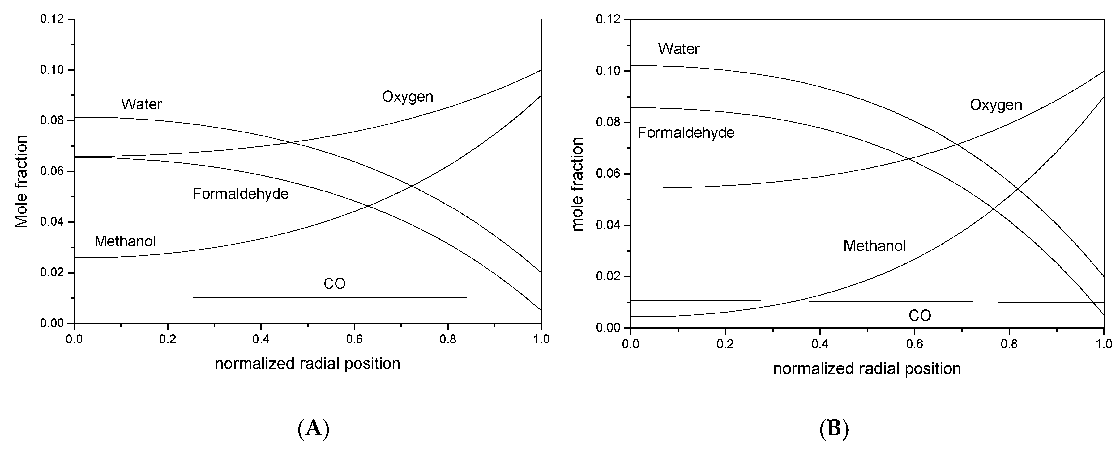
2.7. An Example of Calculation of Effectiveness Factor Complex Reactions

We considered the conversion of methanol to formaldehyde catalyzed by iron–molybdenum oxide catalyst. Two consecutive reactions occur in the process [25]:
C H 3 O H + 1 2 O 2 C H 2 O + H 2 O C H 2 O + 1 2 O 2 C O + H 2 O
The conditions for the reactions, together with catalyst characteristics and other physical parameters [25] used in the calculations, are reported in Table 1.
These reactions follow a redox mechanism, and the most reliable kinetics is the one suggested by Mars and Krevelen [26]:
v = k 1 k 2 P m P O 2 n k 1 P m + k 2 P O 2 n
Different values of n have been suggested in the literature, generally considering n = 1/2 [27] or n = 1 [28]. The inhibition effect of water, formed in both the reactions, can also be introduced in the form of a Langmuir–Hinshelwood term [29], such as
v r = k 1 k 2 P m P O 2 n k 1 P m + k 2 P O 2 n ( 1 1 + b w P w )
Riggs [30] has proposed, on the contrary, pseudo Langmuir–Hinshelwood kinetic laws of the following type:
v r 1 = k 1 P m 1 + a 1 P m + a 2 P w v r 2 = k 2 P f 1 + b 1 P m + b 2 P w
where Pm, Pw, and Pf are, respectively, the partial pressures of methanol, water, and formaldehyde; k1, k2, a1, a2, b1, and b2 are parameters whose values and dependence on temperature is reported Table 2.
The application of the model represented by Equations (57) and (58) to this example was performed with the following assumptions:
-
Catalytic particle is spherical with uniform reactivity, density, and thermal conductivity.
-
The heat of reactions does not change with the temperature.
-
The external diffusion resistance is negligible, and therefore the surface concentration is equal to the one of the bulk.
-
The effective diffusivity has been assumed equal for all the involved chemical species.
The numerical solution of this example was achieved by discretizing the particle radius with 20 internal nodes (Nn = 20). As the reactive mixture is constituted by six different components, we had globally (Nc + 1) Nn = 140 ODEs to be integrated to the stationary state. A further check demonstrated that by increasing the number of internal discretization points brings a negligible variation in the effectiveness factors. As result of this calculation, we obtained the concentration profile of each component inside the catalytic particle, as shown in Figure 9A. By examining this plot, it is clear that the concentration profiles of the reagents methanol and oxygen decreased from the external surface to the center of the pellet, while the opposite occurred for products.
By employing Equation (53), it is possible from these profiles to evaluate the effectiveness factors for each reaction obtaining the following results: η1 = 0.778, η2 = 8.672.
The high effectiveness factor obtained for the second reaction was due to the low concentration of formaldehyde in the bulk gas, in comparison with the formaldehyde concentration accumulated inside the particle, which was significantly higher.
A further result of this example is related to the temperature profile reported in Figure 10. With the reactions being very exothermic, the temperature increased, as expected, from the external surface toward the center, and the overall ΔT was about 3.5 °C. In Figure 10, reported for comparison, are also the same calculations made by adopting the Mars–Krevelen model with the parameters taken from Dente et. al. [28] and Riggs [30].

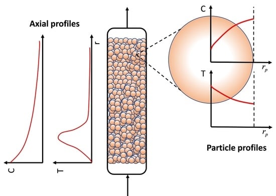
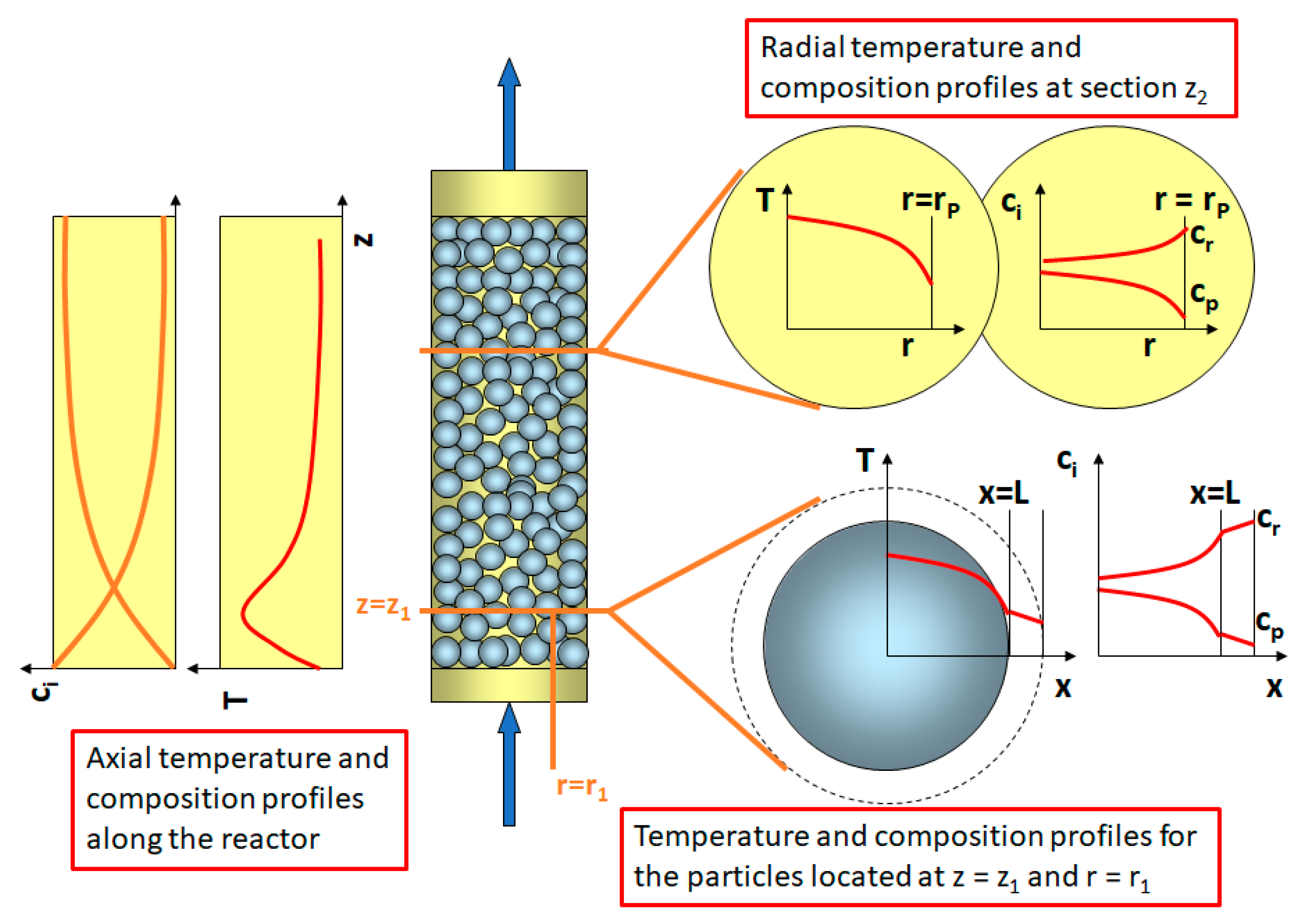
3. Mass and Heat Transfer in Packed Bed Reactors: Long Range Gradients

3.1. Conservation Equations for Fixed-Bed Reactors: Mass and Energy Balances

The generic mass conservation equation for a system of Nc components involved in a reaction network of Nr chemical reactions, related to the I’th component, can be written as in the following equation [16]:
c i t = ( c i u + J i ) + j = 1 N r γ i , j v r , j
where u is the fluid velocity component along various dimensions, ci is the concentration of a generic component, γi,j is the stoichiometric coefficient of chemical species i in reaction j, and vr,j is the j-th rate of reaction based on fluid volume. The quantity Ji represents the molar flux of the i-th component originated by the concentration gradients, temperature gradients, and pressure gradients. The molar flux is in relation with the effective diffusion coefficient Di by Fick’s law, represented by the following equation:
J i = D i c i
Equation (65) is valid in both steady and unsteady state conditions and also contains the accumulation term resulting from the unbalanced difference between input, output, and chemical reactions terms. The overall balance is referred to a suitable control volume.
In the case of a fixed-bed reactor, the control volume assumes the shape of an annulus in a cylindrical coordinate system. By applying the conservation concepts expressed by Equation (65), assuming that only the velocity in the direction of flow (uz = v) is dominant with respect to other directions and as represented in Figure 11, the general Equations (65) and (66) can be combined to give
ε B c i t = z ( u c i ) + z [ D a i c i z ] + 1 r r [ D r i c i r ] + ( 1 ε B ) j = 1 N r e γ i , j v r , j G
where Dai and Dri are the effective dispersion coefficients (diffusivities), in axial and radial directions, for the i-th component. These quantities are referred to the total cross-sectional area perpendicular to the diffusion direction; u is the linear velocity in the catalyst bed and εB is the void fraction of the catalyst bed. The overall reaction rate v r , j G is then multiplied by the factor (1−εB) as the reaction rate is based on the catalyst particle volume.
A simplification can be introduced in Equation (3) by assuming a constant linear velocity in z-direction (reactor axis) and also constant diffusivities along both z and r. Under these assumptions, Equation (67) can be reformulated as follows:
ε B c i t + u c i z D a i 2 c i z 2 D r i [ 2 c i r 2 + 1 r c i r ] = + ( 1 ε B ) j = 1 N r e γ i , j v r , j G
A similar approach can be adopted for the energy balance by replacing in Equation (68) the following quantities: the term ρCpT instead of concentration of chemical species Ci, the effective thermal conductivities K instead of diffusivities D, and reaction enthalpy term (−ΔHj) RGj instead of reaction rate RGj:
ε B T t + u T z K a 2 T z 2 K r [ 2 T r 2 + 1 r T r ] = ( 1 ε B ) ρ C p j = 1 N r e ( Δ H j ) v r , j G
where ρ and CP are the density and specific heat (average values) referred to the gas mixture, respectively.
Considering a fixed-bed reactor, bulk phase concentration and temperature can be regarded, in general, as functions of both r and z coordinates:
c i B = f ( z , r ) T b = g ( z , r )
In the assumptions above, the general mass and energy balance equations for the fixed-bed reactor in which Nr chemical reactions and Nc components are involved are
ε B c i B t + u c i B z D a i 2 c i B z 2 D r i [ 2 c i B r 2 + 1 r c i B r ] = ( 1 ε B ) j = 1 N R γ i , j v r , j G   i = 1 , 2 , N c  
ε B T B t + u T B z K a 2 T B z 2 K r [ 2 T B r 2 + 1 r T B r ] = ( 1 ε B ) ρ C p j = 1 N R ( Δ H j ) v r , j G
Equations (71) and (72) represent a system of PDEs (partial differential equations) for which a solution can be obtained by imposing some suitable boundary conditions related to both variables (temperature and concentration) and their derivatives with respect to z and r. Usual boundary conditions can be written as follows:
T B r = c i B r = 0 at the centerline of the reactor ( r = 0 ) for all z
c i B r = 0   ;   h w ( T B T C ) = ρ C p K r T B r at the wall of reactor ( r = R ) for all z
The first boundary condition (Equation (73)) can be written by considering the symmetry around the axis of the tubular reactor, while the second condition (Equation (74)) expresses the constraint that no mass transfer occurs across the reactor wall. The second part of Equation (74) expresses the zero-accumulation of energy and is related to the heat transfer boundary condition according to which the heat transferred to the cooling fluid, at a temperature Tc, is equal to the heat conducted at the wall.
The axial boundary conditions, written at the reactor inlet, consists of the following equations:
( u c i B ) i n = ( u c i B D a i c i B z ) z = 0 at z = 0 ( u T B ) i n = ( u T B K a T B z ) z = 0
While at the outlet
c i B z = T B z = 0   at   z = Z  
The boundary conditions (Equations (75) and (76)) are based on the flux continuity (both mass and heat) across a boundary, represented by the catalytic bed inlet and outlet.

3.2. External Transport Resistance and Particle Gradients

The link between macroscopical (“long-range”), concentration, and temperature gradients, described by the conservation equations for the entire reactor, and the microscopic situation locally developed around catalytic particles and inside it, is represented by a relation between the overall rate of reaction and the intrinsic kinetic. At a macroscopical level, the observed reaction rate, RGi, represents the rate of mass transfer across an interface between fluid and solid phase, which is ultimately related to the flux at the catalyst particle surface:
j = 1 N r γ i , j v r , j G = k g L ( c i B c i S ) = D e i L c i P x | x = L = j = 1 N r e γ i , j η j v r , j   j = 1 , 2 , , N r
with the following mean of the symbols:
-
kg—gas-solid mass transfer coefficient (film);
-
L—characteristic length of particle (radius for spherical pellets);
-
ciS—surface concentration of component i;
-
ciP—particle internal concentration of component i;
-
Dei—effective diffusivity of component i into the particle;
-
x—particle radial coordinate;
-
ηj—effectiveness factor for reaction j;
-
vr,j—intrinsic rate of reaction j.
In a similar way, we can write a relation for the thermal flux:
j = 1 N r ( Δ H j ) v r , j G = h L ( T S T b ) = K e f f L T P x | x = L
where
-
h—film heat transfer coefficient;
-
TS—temperature at the surface of the pellet;
-
TP—temperature inside the pellet;
-
Keff—effective thermal conductivity of the catalytic particle.
By considering Equation (77), the relationship between the rate of reaction at a macroscopic level and the intrinsic reaction rate is expressed for each chemical reaction by the effectiveness factor η or, in an equivalent way, by means of the concentration gradients measured at the particle surface. This consideration evidences the necessity to solve mass and energy balance equations related to catalytic particles to calculate local (microscopic) concentration and temperature profile. This calculation must be replicated, in principle, in each position along the reactor.
Conservation equations for the particles can be written as in the following equations (Equations (79) and (80)):
ε P c i P t = D e i [ 2 c i P x 2 + 2 x c i P x ] ρ P j = 1 N r γ i , j r c j   i = 1 , 2 , , N c
ε P ρ P C P P T P t = K e [ 2 T P x 2 + 2 x T P x ] ρ P j = 1 N r ( Δ H j ) r c j
with the following meanings of the symbols:
-
εP—catalytic particle void fraction;
-
ρP—catalytic particle density;
-
CPP—catalytic particle specific heat.
The simultaneous solution of PDE system represented by Equations (79) and (80) can be obtained by imposing some boundary conditions that are valid at the center and at the external surface of the catalyst particle respectively. These boundary conditions can be derived from symmetry consideration and from continuity related to both concentration and temperature:
c i P x = 0 T P x = 0 at r = 0 ( center ) c i P = c i S   T P   =   T S at r = L ( surface )
As it was defined, the problem consists in a set of non-linear partial differential equations (PDEs) that must be solved at two levels: the first is a local level, related to a single catalytic particle, and the second is a long-range scale for the entire reactor. The solution of the problem in the full form, expressed by the Equations (72) to (79), is a complex task, even by adopting sophisticated numerical solution algorithms, while an analytical exact solution is impossible for the mostly practical cases. In the following part of this review, an overview of the possible simplifications is presented and some simplified equations are reported in association with problems much easier to solve.

3.3. Conservation Equations in Dimensionless Form and Possible Simplification

A convenient way to introduce the mentioned simplifications is in rewriting mass and energy balances for the reactor in a dimensionless form. This strategy has both the scope to emphasize some parameters of the reactor and the ability to implement a more robust procedure for the numerical solution.
We can pose
n d = Z d P   m d = R d P   A d = Z R θ d = Z u c ¯ i = c i B c i B ( i n ) T ¯ = T B T B ( i n ) r ¯ = r R r z ¯ = z Z t ¯ = t θ d
with
-
dP—particle diameter;
-
R—fixed-bed reactor radius;
-
Z—fixed-bed reactor length;
-
cB(in)i—reactor inlet concentration;
-
TB(in)—reactor inlet temperature.
Within these assumptions, the reactor conservation equations become
ε B c i ¯ t + c i ¯ z ¯ 1 n d P m a 2 c i ¯ z ¯ 2 1 m d P m r [ 2 c i ¯ r ¯ 2 + 1 r ¯ c ¯ i r ¯ ] = ( 1 ε B ) θ d c i B ( i n ) j = 1 N r e γ i , j v r , j G   i = 1 , 2 , , N c
ε B T ¯ t ¯ + T ¯ z ¯ 1 n d P h a 2 T ¯ z ¯ 2 A d m d P h r [ 2 T ¯ r ¯ 2 + 1 r ¯ T ¯ r ¯ ] = ( 1 ε B ) θ d ρ C p T B ( i n ) j = 1 N r e ( Δ H j ) v r , j G
In the Equations (83) and (84), we can recognize some fundamentals dimensionless groups that are related to mass dispersion, which is related to axial and radial directions, represented by Peclet’s numbers expressed by the following equations:
P m a = d P u D a   ( axial )   P m r = d P u D r   ( radial )  
and analogously for heat dispersion we have
P h a = d P u k a   ( axial )   P h r = d P u k r   ( radial )  
The quantitative criteria that can be adopted to determine if the dispersion phenomena affect the overall reactor performances are Peclet’s numbers and reactor-to-particle size ratios (n, m, and A). Moreover, these criteria can give indications to decide whether or not some simplifications are allowed. The operative conditions adopted and chemical reaction characteristics can suggest further simplifications according to which mass and energy conservation equations can be solved in a simplified form. The first and more common simplification is represented by the steady state, allowing the elimination of time variable and all its derivatives, in the left-hand sides of Equations (71), (72), (79), and (80). From an energetic point of view, the reaction enthalpy also plays a very important role. When the reaction heat is negligible or very low, the reactor can be run isothermally, and then, with the temperature being a constant, the heat balance equation can be eliminated. If the reactor is thermally insulated from the environment, it is operated in adiabatic conditions, as many reactors are in practice. In this case, radial gradients could be negligible, and therefore only a one-dimensional model is sufficient for the description of the reactor behavior. An intermediate situation, comprising these two limit cases described, is represented by a reactor working in conditions that cannot be considered isothermal nor adiabatic. This is the case of very exothermal reactions for which an external cooling system is required in order to guarantee the safety of the reactor and to preserve the catalyst durability. In this case, a numerical solution of conservation equations in full form appears to be the only feasible strategy. However, the conservation equations can still be applied in a simplified form, even if the problem remains complex to solve and is more difficult with respect to the two limit cases (isotherm and adiabatic) cited previously. Normally, for an extremely exothermic chemical reaction, the packed beds with small diameter are used for promoting the heat removal, and in this case the radial temperature profile can be neglected. The problem is again mono-dimensional in this case. In general, according to Carberry [31], the gradients along the reactor radius, for practical purposes, can be neglected when the radial aspect ratio m = R/dp is less than 3 or 4. Further guidelines can be gained by examining the values of Peclet’s numbers and the reactor aspect ratios; as an example, the axial aspect ratio n=Z/dP is usually very large, and considering that Pma is about 2 for gases flowing through a catalytic bed for Reynold’s number (based on particle diameter) greater than 10, then the term nPma is also large, revealing that axial mass dispersion can be almost completely neglected. Table 3 [32] summarizes the general guidelines to introduce principal simplifications in the mass balance for a packed-bed reactor operating under stationary conditions; the two limit cases are also reported with concern to the isothermal and adiabatic reactor together with the intermediate situation in which the reactor cannot be considered isothermal nor adiabatic.

3.4. Examples of Applications

In the following sections, we examine some examples concerning fixed-bed reactors operating in the various possible thermal regimes.

3.4.1. Isothermal Conditions

Isothermal conditions are seldom obtained in industrial packed bed reactors and are only for systems with a very low heat of reaction, whereas they are most commonly encountered in slurry reactors because liquid phase has a high thermal conductivity. Therefore, in these cases, we can have only internal, and sometimes external, diffusion limitation to the reaction.

3.4.2. Adiabatic Conditions

If the reactor is operated so that heat transfer to the surrounding is negligible, the system could be considered in adiabatic conditions. For simplicity, we can consider a system of a single reaction, AP, in steady state adiabatic conditions, and then the material energy balances for a tubular reactor with no axial and radial dispersion could be derived from Equations (69) and (70), resulting in the following expressions:
d F A d z = ρ B A R ¯ 1 d T d z = ρ B G C P ( Δ H 1 ) R ¯ 1
where
-
G—mass velocity;
-
cross section of the reactor tube;
-
FA, F0A component molar flow rate;
-
R j ¯ —reaction rate for reaction j based on catalyst mass.
In the above equations, it is convenient to introduce the fractional conversion, XA, obtaining the following equations:
d X A d z = ρ B A F A 0 R ¯ 1 d T d z = ρ B G C P ( Δ H 1 ) R ¯ 1
Dividing Equations (87) and (88) term by term, we obtain an expression relating the conversion and the temperature:
d X A d T = A G C P F A 0 ( Δ H 1 )   or   in   integrated   form :   X A = α A + β A T  
with αA and βA as constants. The main result expressed by the previous equation is that a linear relationship exists between the temperature and the conversion for an adiabatic reactor.
Adiabatic reactors are frequently employed in industrial practice, especially in the case of equilibrium reactions for which the desired conversion is achieved through assembling the reactor in a series of adiabatic catalytic beds provided with intermediate heat removal or supplying system in accordance with the reaction being exothermic or endothermic. Figure 12 and Figure 13 report a schematic reactor configuration for an exothermic and an endothermic reaction, respectively, together with temperature-conversion diagrams that show conversion equilibrium curves and straight lines resulting from balance Equation (89) and cooling or heating. With such an arrangement, it is possible to achieve good control over the final conversion of reversible reactions by controlling the temperature at the outlet of each catalytic bed. In the diagrams reported in Figure 12 and Figure 13, dashed lines represent cooling or heating operations.

4. Non-Isothermic and Non-Adiabatic Conditions

4.1. Conversion of o-Xylene to Phthalic Anhydride

Let us consider, first of all, a reaction that is performed in a packed-bed tubular reactor, operated in an modality non-isothermal and non-adiabatic that consists in the synthesis of phthalic anhydride (PA) obtained by oxidation of o-xylene (OX) with oxygen (O). A simplified scheme for this oxidation reaction can be expressed as follows:
Processes 08 01599 i002
The reaction is catalyzed by vanadium pentoxide supported on α-alumina and has a high exothermal character. From Equation (90), it is evident that the reaction can lead to CO2 and CO production, if not properly thermally controlled, giving a low yield in PA. For the reactor simulation, therefore, thermal effect must be taken into account for both the reaction and the heat exchanged with the cooling medium. The kinetic equations and related parameters for the reactions (Equation (90)) are reported in Table 4, together with the characteristics of the reactor and of the catalytic particles used in the simulations [33].
A specific characteristic of this reactor is the catalyst dilution with an inert material in the first part of the reactor (0.75 m) that is realized at the purpose of an improved temperature control.
For the model development, some basic assumptions should be stated, as in the following points:
  • No axial and radial dispersion;
  • No radial temperature and concentration gradients in the reactor body;
  • Plug flow behavior of the reactor;
  • No limitation related to internal diffusion in catalytic particles.
The assumptions related to radial profiles can be supported by the criteria expressed in Table 3 for radial aspect ratio m=R/dp that can be estimated as m = 4.1 and then slightly above the limit. By considering the assumptions and simplifications applied to this system, we can write a material balance equation directly from Equation (69) considered in the stationary state:
d F i d z = F d y i d z = ρ B π D r 2 4 j = 1 N r γ i , j R ¯ j ( 1 + m I ) i = 1 , 2 , , N c  
assuming a constant molar flow rate F, and with the following substitution:
u = Q A   Qc i = F i   A = π D r 2 4 F i = y i F
where:
-
Q—volumetric overall flow rate;
-
A—cross section of the reactor tube;
-
Dr—reactor diameter;
-
Fi—component molar flow rate;
-
yi—mole fraction of component i;
-
mI—mass of inert per unit mass of catalyst (dilution ratio);
-
R j ¯ —reaction rate for reaction j based on catalyst mass.
The heat is constituted by Equation (72) and can be modified in a way similar to that adopted for mass balance and according to the absence of radial profiles and to the heat exchange of external cooling fluid in the reactor jacket. The thermal exchange with the surrounding (thermal fluid into the jacket) cannot be considered only as a boundary condition but as a separate term in the energy balance equation. A behavior similar to that of a double pipe heat exchanger (see Figure 14) can be adopted for the reactor and then, referring to a unit of reactor volume, the heat transferred across the external surface is defined as
q = U ( T C T ) π D r d z A d z = U ( T C T ) π D r A = 4 U ( T C T ) D r
Equation (93) represents an additional term in the energy balance, and must be added to the heat associated with the reaction, resulting in the following overall differential equation for temperature evolution along the reactor axis:
d T d z = ρ B G C P j = 1 N r ( Δ H j ) R ¯ j ( 1 + m I ) + 4 U D G C P ( T C T )
with G = F · M F A , with the following meanings for the symbols:
-
G—mass velocity;
-
MF—average molecular weight of mixture.
The system of differential Equations (91) and (94) can be integrated in axial direction, z, for the calculation of temperature and composition profiles. The temperature profile resulting from this mono-dimensional model (axial coordinate) is reported in Figure 15 [33], with this diagram also reporting, as a comparison, the result of a more complex bi-dimensional model in which profiles in a radial direction are also taken into account.
As was shown before, the bi-dimensional model involves the solution of partial differential equations. In the considered example is the numerical strategy of finite differences method (FDM). The two models (one and two dimensions) give comparable results for what concerns axial temperature profiles. A conclusion is that the one-dimensional model can be considered sufficiently accurate for many practical purposes. The bi-dimensional model, however, foresees a slightly higher conversion to CO and CO2, due to the higher temperature along the reactor.

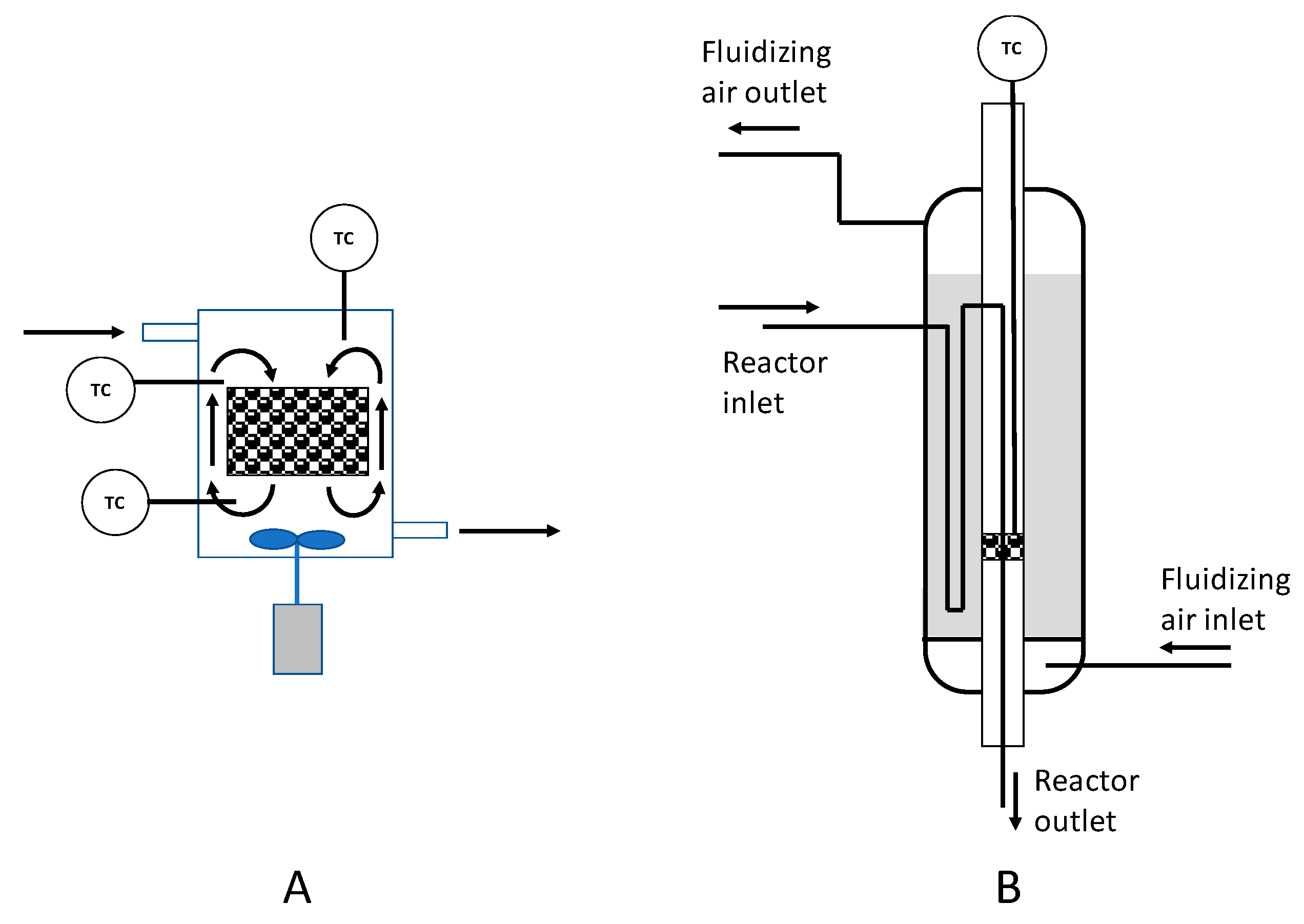
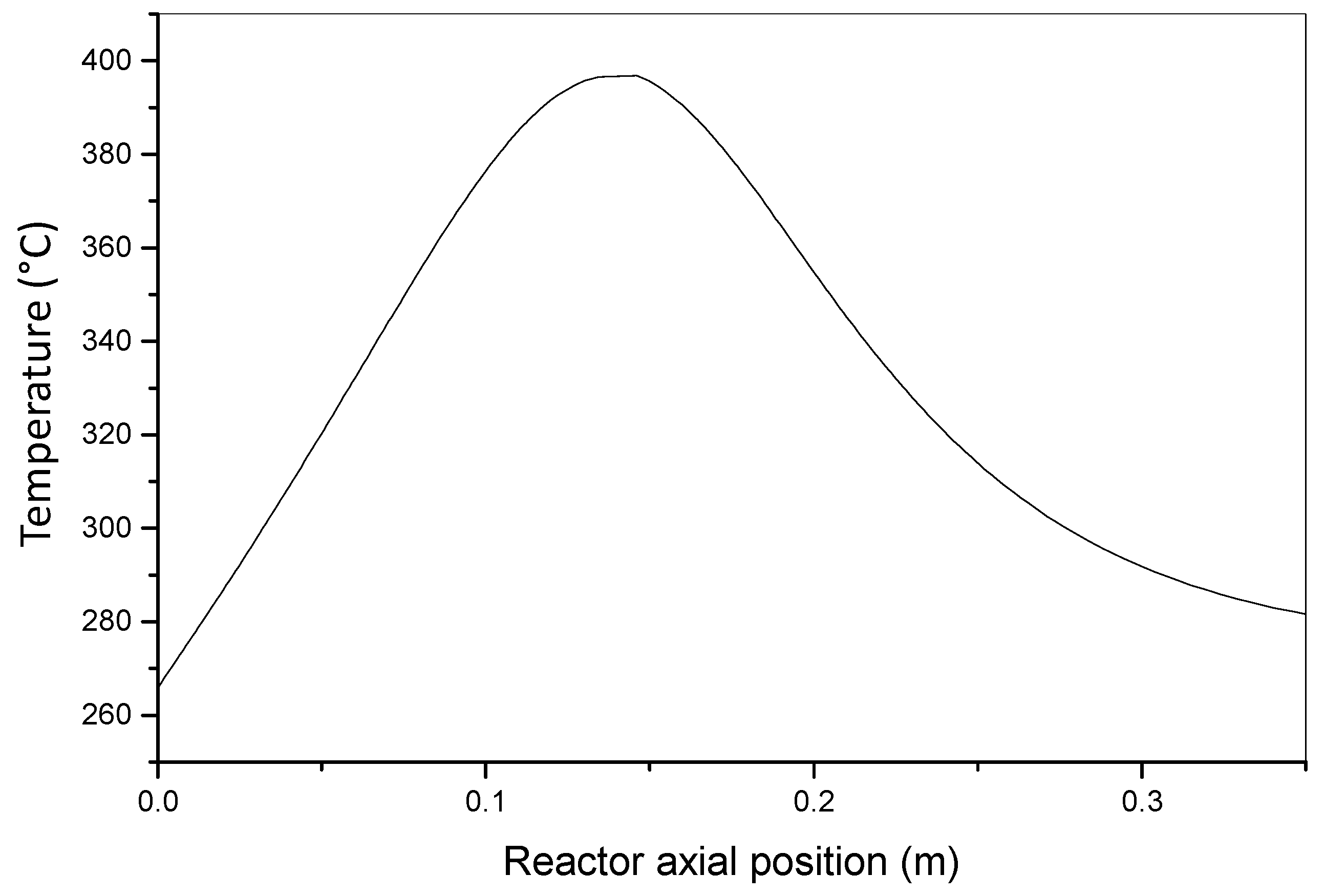
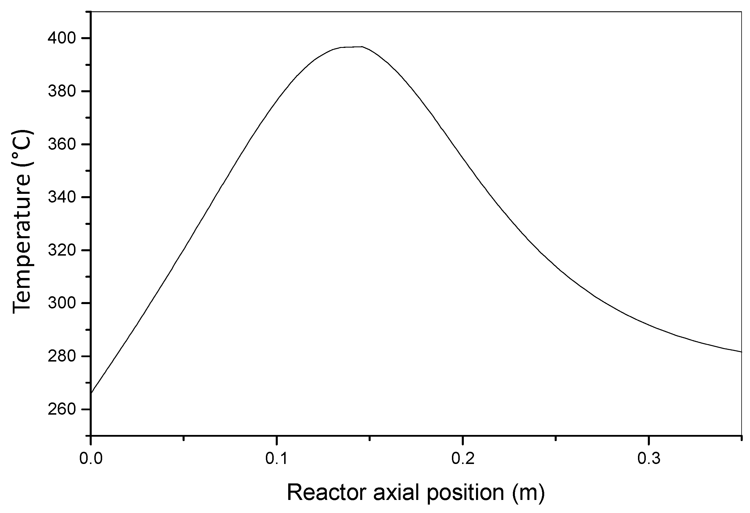
4.2. Conversion of Methanol to Formaldehyde

As a further example of a system that cannot be considered isothermal nor adiabatic, we chose the same reaction previously adopted in Section 2.7 for the evaluation of the effectiveness factor in a non-isothermal pellet, that is, the catalytic conversion of methanol to formaldehyde. Two reactions occurred as seen previously (Equation (61)).
These reactions were performed in a tubular reactor packed with catalyst and equipped with a jacket in which a heat transfer fluid is circulated with the purpose to a better temperature control. Table 5 reports the reactor operating conditions and other characteristics. A simulation was performed by using these conditions and the kinetic data from Riggs [29] (details were reported in [25]), obtaining composition and temperature profiles along the reactor axis. In this case study, a further aspect was introduced into the model, consisting in the calculation of the catalyst effectiveness factor along the reactor, considering diffusional limitations inside the particles.
Some simplifying assumptions were introduced in the present case for the model development in a way similar to that of the example reported in the previous section:
  • Negligible dispersion in axial and radial directions;
  • Absence of concentration and temperature profiles along the reactor radius;
  • Plug flow reactor behavior.
By applying the criteria of Table 3, radial profiles can be considered negligible as the aspect ratio in radial direction was m = R/dP = 3.6, which was well below the limit value of 4. Under these assumptions, the resulting model is mono-dimensional because it only considers axial reactor profiles. At each location along the reactor axis, an effectiveness factor calculation was performed to obtain the value of the reaction rate that is related to that point, determining, in this way, an effectiveness factor axial profile. On the basis of the described assumptions and introducing molar flow rates relative to each chemical component, we can express material balance equations by the following model:
d F i d z = ρ B π D r 2 4 j = 1 N r γ i , j R ¯ j i = 1 , 2 , , N c
u = Q A Q c i = F i A = π D r 2 4
that can be derived upon the following substitution in Equation (71):
The energy balance, represented by Equation (72), can also be simplified, as done for the mass balance, according to the assumed absence of radial profiles and to the presence of reactor jacket with cooling fluid, as reported, for example, in Session 4.1. The heat exchanged per unit of reactor volume between the reactor and the cooling jacket can be defined as follows:
q = U ( T C T ) π D r d z A d z
This term must be added algebraically to the reaction enthalpy term in the heat balance equation, yielding the following expression:
( i = 1 N c F i C P i ) d T d z = π D r 2 4 ρ B j = 1 N r ( Δ H j ) R ¯ j + π D r U ( T C T )
Equations (95) and (98) represent a system of Nc+1 coupled ordinary differential equations that must be integrated along the z axial direction to calculate the desired profiles of composition and temperature. At each integration step along z, a calculation of the effectiveness factor for each chemical reaction must be performed according to the procedure described in Session 2.6. A suitable integration algorithm must be adopted with a variable z step size, inversely proportional to the axial derivative dT/dz, so that a smaller step size is used when a steep temperature increase is detected in correspondence to a steeper profile. Figure 16 reports the axial temperature profile as a result of this simulation. This figure shows that the reaction mixture fed to the reactor undergoes a steep increase in gas temperature due to the strong exothermic character of this reactive system.
As methanol conversion proceeds (see composition profile reported in Figure 17), the main reaction rate also decreases, and the same trend can be appreciated for the temperature. Finally, in Figure 18, the profiles of the effectiveness factors for the two reactions is reported. It is interesting to observe that the main reaction is characterized, in the first part of the reactor, by an effectiveness factor much higher than unity, with this indicating that catalytic particles are not isothermal and a temperature profile is developed inside them.

5. Conclusions

The role of heat and mass transfer in affecting the kinetic studies in gas–solid tubular reactors was discussed in detail by surveying the abundant literature published on the subject. All the occurring phenomena were described and the equations for their interpretation were given.
Considering the enormous progress of electronic computers, many problems that were intractable in the past for their mathematical complexity can today be easily and rigorously solved with numerical approaches. For more clarity, some examples of mathematical solutions were reported.

Author Contributions

E.S. wrote the first part of the work related to the heat and mass transfer in the single pellet. R.T. wrote the second part related to the long-range gradients in packed bed reactors. All authors have read and agreed to the published version of the manuscript.

Funding

Thanks are due to Eurochem Engineering LtD for funding the work.

Conflicts of Interest

The authors declare no conflict of interest.

Glossary

List of Symbols
amSpecific surface area
AReactor cross section
bwWater adsorption equilibrium constant
cGeneric concentration
ciConcentration of component i
ci°Initial i concentration
cbGeneric concentration of a component in the bulk
ciBConcentration of i in the bulk
ciPConcentration of i inside a catalytic particle
cSGeneric concentration at the catalytic surface
ciSConcentration of i at the surface
CpAverage gas specific heat
CpPParticle specific heat
ΔcConcentration gradient
ΔcminMinimum concentration gradient
DReactor diameter
dpParticle diameter
DGeneric molecular diffusivity
DiMolecular diffusivity of component i
Di,jMutual binary diffusion coefficient
D12Mutual binary diffusion coefficient
DimDiffusion coefficient of i in a mixture m
Deff Effective molecular diffusivity
(Di)effEffective molecular diffusivity of component i
DbeBulk diffusion coefficient
DkeKnudsen diffusion coefficient
DeiEffective diffusivity inside particle
DaiAxial diffusivity of component i
DriRadial diffusivity of component i
FiMolar flow rate of component i
FOverall molar flow rate
GMass velocity
hFilm heat transfer coefficient
hwWall heat transfer coefficient
ΔHGeneric reaction enthalpy
ΔHjEnthalpy of reaction j
JiMolar flux of component i
JD, JHTerms for mass and heat transfer analogy
k, kiGeneric kinetic constant
kBBoltzmann’s constant
kTGeneric thermal conductivity of the fluid
kfThermal conductivity of the bulk
keffEffective thermal conductivity
kSolThermal conductivity of the solid
KaAxial thermal conductivity
KrRadial thermal conductivity
KeParticle thermal conductivity
kSKinetic constant
kcFilm mass transfer coefficients (concentration gradient)
kgFilm mass transfer coefficients (pressure gradient)
kmMass transfer coefficient
LCharacteristic length
LeLewis’s number
mRadial aspect ratio
mIInert dilution ratio
M, MiMolecular weight
MFAverage molecular weight of the mixture
MwWeisz modulus
NCNumber of components
NreNumber of reactions
NrMolar flux
Ni, NAMolar flux
NNumber of nodes
nReaction order
PTotal pressure
PmMethanol partial pressure
PfFormaldehyde partial pressure
PwWater partial pressure
PO2Oxygen partial pressure
PmaAxial Peclet’s number for mass
PmrRadial Peclet’s number for mass
PhaAxial Peclet’s number for heat
PhrRadial Peclet’s number for heat
PrPrandtl’s number
QRate of heat transfer
QvOverall volumetric flow rate
qHeat flux
rReactor radial coordinate
rPParticle spherical radius
RGas constant
RrReactor radius
RniReaction rate at node i
RjReaction rate (fluid volume)
R j ¯ Reaction rate (catalyst mass)
rcjIntrinsic reaction rate
ReReynold’s number
SvSpecific surface area
ShSherwood’s number
ScSchmidt’s number
SSelectivity
SgSpecific surface area
TGeneric temperature
TSTemperature at particle surface
TPTemperature inside the particle
TbBulk temperature
TcCooling fluid temperature
ΔTmaxMaximum temperature difference
tTime
uVelocity
uzVelocity in z direction
UOverall heat transfer coefficient
vrReaction rate
vr,iReaction rate, reaction i-th
vr,jGReaction rate (pellet volume)
VciCritical volume of component i
xParticle radial coordinate
XiFractional conversion
yiGas phase mole fraction component i
zAxial reactor coordinate
ZReactor length
Greek Letters
αAConstant in Equation (89)
αBConstant in Equation (89)
αEReaction rate exponential parameter
αJConstant in Equation (38)
αHConstant in Equation (40)
βPrater’s number
βJConstant in Equation (38)
βHConstant in Equation (40)
γdrDimensionless concentration
γijStoichiometric coefficient
δThickness of boundary layer
εdrDimensionless radius
εBBed void fraction
εBsBed void fraction of the solid
εJConstant in Equation (38)
εHConstant in Equation (40)
εijInteraction parameter
εpParticle void fraction
η, ηjEffectiveness factor
µViscosity
θPorosity of the solid
ρAverage gas density
ρpParticle density
ρdIntermolecular distance
σijKinetic diameter
τTortuosity factor
ϕThiele modulus
ϕLJLennard–Jones potential
ydrDimensionless reaction rate
DCollision integral
Nabla operator

References

  1. Santacesaria, E.; Tesser, R. The Chemical Reactor from Laboratory to Industrial Plant; Springer: Berlin, Germany, 2018. [Google Scholar]
  2. Froment, G.F. The kinetics of complex catalytic reactions. Chem. Eng. Sci. 1987, 42, 1073–1087. [Google Scholar] [CrossRef]
  3. Smith, J.M. Chemical Engineering Kinetics; McGraw-Hill: New York, NY, USA, 1981. [Google Scholar]
  4. Fogler, H.S. Elements of Chemical Reaction Engineering; Prentice-Hall International: Upper Saddle River, NJ, USA, 1986. [Google Scholar]
  5. Horak, J.; Pasek, J. Design of Industrial Chemical Reactors from Laboratory Data; Hayden Publishing: London, UK, 1978. [Google Scholar]
  6. Satterfield, C.N.; Sherwood, T.K. The Role of Diffusion in Catalysis; Addison-Wesley Publishing: Boston, MA, USA, 1963. [Google Scholar]
  7. Levenspiel, O. The Chemical Reactor Omnibook; OSU Book Store: Corvallis, OR, USA, 1984. [Google Scholar]
  8. Satterfield, C.N. Heterogeneous Catalysis in Practice; Addison-Wesley Publishing: Boston, MA, USA, 1972. [Google Scholar]
  9. Holland, C.D.; Anthony, R.G. Fundamentals of Chemical Reaction Engineering; Prentice-Hall: London, UK, 1979. [Google Scholar]
  10. Westerterp, K.R.; van Swaaij, W.P.M.; Beenackers, A.A.C.M. Chemical Reactor Design and Operation; John Wiley & Sons: New York, NY, USA, 1984. [Google Scholar]
  11. Davis, M.E.; Davis, R.J. Fundamentals of Chemical Reaction Engineering; Dover Publications, Inc.: New York, NY, USA, 2003. [Google Scholar]
  12. Vogel, G.H. Process Development Wiely—VCH; John Wiley & Sons: Weinheim, Germany, 2005. [Google Scholar]
  13. Winterbottom, J.M.; King, M.B. Reactor Design for Chemical Engineers; Stanley Thornes Ltd.: Cheltenham Glos, UK, 1999. [Google Scholar]
  14. Wheeler, A. Reaction rates and selectivity in catalyst pores. In Advances in Catalysis; Academic Press: Cambridge, MA, USA, 1951; Volume 3. [Google Scholar]
  15. Bird, R.B.; Stewart, W.E.; Lightfoot, E.N. Fenomeni di Trasporto; Casa Editrice Ambrosiana: Milan, Italy, 1970. [Google Scholar]
  16. Missen, R.W.; Mims, C.A.; Saville, B.A. Chemical Reaction Engineering and Kinetics; John Wiley & Sons: New York, NY, USA, 1999. [Google Scholar]
  17. Carberry, J.J. Physico chemical aspects of mass and heat transfer in heterogeneous catalysis. In Catalysis; Springer: Berlin/Heidelberg, Germany, 1987; pp. 131–171. [Google Scholar]
  18. Thiele, E.W. Relation between catalytic activity and size of particle. In Industrial and Engineering Chemistry; ACS Publications: Washington, DC, USA, 1939; Volume 31, pp. 916–920. [Google Scholar]
  19. Weisz, P.B.; Prater, C.D. Interpretation of measurements in experimental catalysis. In Advances in Catalysis; Academic Press: New York, NY, USA, 1954; Volume 6, pp. 143–196. [Google Scholar] [CrossRef]
  20. Santacesaria, E. Catalysis and transport phenomena in heterogeneous gas-solid and gas-liquid-solid systems. In Catalysis Today; Elsevier Science: Amsterdam, The Netherlands, 1997; Volume 34, pp. 411–420. [Google Scholar]
  21. Froment, G.F.; Bishoff, K.B. Chemical Reaction Analysis and Design; John Wiley & Sons: New York, NY, USA, 1990. [Google Scholar]
  22. Woodside, W.W.; Messner, J.H. Thermal conductivity of porous media. J. Appl. Phys. 1961, 32, 1688. [Google Scholar] [CrossRef]
  23. Hindmarsh, A.C. LSODE and LSODI, two initial value ordinary differential equation solvers. ACM Signum 1980, 15, 10–11. [Google Scholar] [CrossRef]
  24. Palm, W.J. Introduction to MATLAB for Engineers; Mc Graw-Hill: New York, NY, USA, 2011. [Google Scholar]
  25. Tesser, R.; Santacesaria, E. Catalytic oxidation of methanol to formaldehyde: An example of kinetics with transport phenomena in a packed -bed reactor. Catal. Today 2003, 77, 325–333. [Google Scholar] [CrossRef]
  26. Mars, J.; Krevelen, D.W. Oxidations carried out by means of vanadium oxide catalysts. Chem. Eng. Sci. 1954, 3, 41. [Google Scholar] [CrossRef]
  27. Santacesaria, E.; Morbidelli, M.; Carrà, S. Kinetics of the catalytic oxidation of methanol to formaldehyde. Chem. Eng. Sci. 1981, 36, 909–918. [Google Scholar] [CrossRef]
  28. Dente, M.; Collina, A.; Pasquon, I. Verifica di un reattore tubolare per l’ossidazione del metanolo a formaldeide. La Chimica Industria 1966, 48, 581–588. [Google Scholar]
  29. Riggs, J.B. Introduction to Numerical Methods for Chemical Engineers; Texas Tech University Press: Lubbock, TX, USA, 1988. [Google Scholar]
  30. Carrà, S.; Forzatti, P. Engineering aspects of selective hydrocarbons oxidation. Catal. Rev. Sci. Eng. 1977, 15, 1–52. [Google Scholar] [CrossRef]
  31. Carberry, J.J. Chemical and Catalitic Reaction Engineering; McGraw-Hill: New York, NY, USA, 1976. [Google Scholar]
  32. Lee, H.H. Heterogeneous Reactors Design; Butterwoth Publisher: Oxford, UK, 1984. [Google Scholar]
  33. Froment, G.F. Fixed bed catalytic reactors—Current design status. Ind. Eng. Chem. 1967, 59, 18–27. [Google Scholar] [CrossRef]
Figure 1. Overview of temperature and concentration macroscopic and microscopic gradients in packed bed reactor (taken and adapted from [1]). Reprinted with the permission of Springer, Copyright 2018.
Processes 08 01599 g001
Figure 2. Examples of “gradientless” laboratory reactors. (A) Continuous stirred tank reactor (CSTR); (B) fixed-bed reactor.
Processes 08 01599 g002
Figure 3. Profiles of concentration and temperature in a spherical catalytic particle.
Processes 08 01599 g003
Figure 4. Reference scheme for mass and heat balance related to a catalyst particle.
Processes 08 01599 g004
Figure 5. (A) Relationship between effectiveness factor and Thiele modulus; (B) relationship between effectiveness factor and Weisz modulus. Re-elaborated from Santacesaria [20] with the permission of Elsevier-Catalysis Today 1997.
Processes 08 01599 g005
Figure 6. Effectiveness factor versus Thiele modulus for different order of reaction. Re-elaborated from Froment and Bischoff [21].
Processes 08 01599 g006
Figure 7. Effectiveness factors against the Thiele modulus in the case of both exothermic and endothermic reactions with an internal temperature gradient. Re-elaborated from Santacesaria [20] with the permission of Elsevier-Catalysis Today 1997.
Processes 08 01599 g007
Figure 8. Scheme of the experimental device for the determination of effective diffusivity of a catalyst pellet.
Processes 08 01599 g008
Scheme 1. Scheme of discretization.
Processes 08 01599 sch001
Figure 9. Mole fraction profiles inside a catalytic particle. (A) Kinetics of Riggs [30]; (B) kinetics of Dente et al. [28].
Processes 08 01599 g009
Figure 10. Internal temperature profile for a catalytic particle obtained with different kinetic models.
Processes 08 01599 g010
Figure 11. Scheme of the coordinate system and control volume for the fixed-bed conservation equations.
Processes 08 01599 g011
Figure 12. Scheme of a multistage adiabatic reactor (exothermic reaction). (left) reactor setup; (right) temperature profile.
Processes 08 01599 g012
Figure 13. Scheme of a multistage adiabatic reactor (endothermic reaction). (left) reactor setup; (right) temperature profile.
Processes 08 01599 g013
Figure 14. Double-pipe countercurrent reactor.
Processes 08 01599 g014
Figure 15. Comparison of the results of the one- and bi-dimensional models for reactor simulation (elaborated from data reported by Froment [33], see also [1]).
Processes 08 01599 g015
Figure 16. Axial temperature profile.
Processes 08 01599 g016
Figure 17. Axial profiles for component mole fractions.
Processes 08 01599 g017
Figure 18. Axial profiles for the effectiveness factor for the two reactions.
Processes 08 01599 g018
Table 1. Physico-chemical data for the calculation.
Ke = 2.72 × 10⁻⁴KJ/(s m K)effective thermal conductivity
De = 1.07 × 10⁻⁵ exp(-672/T)m2/seffective diffusivity
ρP = 1180Kg/m3particle density
Cp = 2.5KJ/(mole K)particle specific heat
P = 1.68atmtotal pressure
TS = 539Ksurface temperature
dP = 3.5 × 10⁻³mparticle diameter
Bulk gas compositionmol%
CH3OH9.0
O210.0
CH2O0.5
H2O2.0
CO1.0
N277.5
Table 2. Kinetic parameters for the model.
k1 = 5.37 × 10² exp(-7055/T)
k2 = 6.42 × 10⁻⁵ exp(-1293/T)
a1 = 5.68 × 10² exp(-1126/T)
a2 = 8.37 × 10⁻⁵ exp(7124/T)
b1 = 6.45 × 10⁻⁹ exp(12,195/T)
b2 = 2.84 × 10⁻³ exp(4803/T)
ΔH1 = 37,480 cal/mole
ΔH2 = 56,520 cal/mole
Table 3. Guidelines for simplifications in the left-hand side of conservation equations, with reference to stationary conditions.
Reactor ConditionsAspect Ratio CriteriaLeft-Hand Side of Equations (71) and (72)
Isothermal u c B i z
Adiabatic ( Z d P ) ( d P D a ) > 300 R e > 10 u c B i z ρ C P u T B z
( Z d P ) ( d P D a ) < 300 R e > 10 u c B i z { ρ C P u T B z   or ,   if   necessary ρ C P u T B z K a 2 T B z 2
Non-isothermal and non-adiabatic R r d P > 4 u c B i z D r ( 2 c B i r 2 + 1 r c B i r ) ρ C P u T B z K r ( 2 T B r 2 + 1 r T B r )
R r d P 4   R e > 30 u c B i z ρ C P u T B z
Table 4. Kinetic data for the conversion of o-xylene to phthalic anhydride.
r1 = k1 POX PO (Kmol/Kg-cat h)ln k1= −27,000/RT + 19.837
r2 = k2 PPA PO (Kmol/Kg-cat h)ln k2= −31,000/RT + 20.860
r3 = k3 POX PO (Kmol/Kg-cat h)ln k3= −28,600/RT + 18.970
ΔH1 = −307 Kcal/mol
ΔH2 = −783 Kcal/mol
ΔH3= −1090 Kcal/mol
U = 82.7 Kcal/ m2 h °Coverall heat transfer coefficient
D = 0.025 mreactor diameter
Z = 3 mreactor length
dP = 0.003 mparticle diameter
CP = 0.25 Kcal/Kg °Caverage specific heat
ρB =1300 Kg/m3bulk density of the bed
Feed composition:yOX = 0.0093
yO = 0.208
Feed molar flow rateF = 0.779 moles/h
Inert dilution of the catalystmI =0.5 for the first quarter
Inlet temperatureT0 = 370 °C
Table 5. Reactor characteristic and operating conditions.
Inlet temperature539 K
Total pressure1.68 atm
Bulk density of the bed0.88 Kg/m3
Overall heat transfer coefficient U0.171 KJ/(m2 s K)
Heating medium temperature544 K
Reactor diameter2.54 x 10−2 m
Particles diameter3.5 x 10−3 m
Reactor length0.35 m
Gas inlet composition mol %
CH3OH9
O210
CH2O0.5
H2O2
CO1
N277.5
Publisher’s Note: MDPI stays neutral with regard to jurisdictional claims in published maps and institutional affiliations.

