Abstract
The internal recirculation plays an important role in different areas of the biological treatment of wastewater treatment plants because it has a great influence on the concentration of pollutants, especially nutrients. A usual manipulation of the internal recirculation flow rate is based on the target of controlling the nitrate concentration in the last anoxic tank. This work proposes an alternative for the manipulation of the internal recirculation flow rate instead of nitrate control, with the objective of avoiding limit violations of nitrogen and ammonia concentrations and reducing operational costs. A fuzzy controller is proposed to achieve it based on the effects of the internal recirculation flow rate in different areas of the biological treatment. The proposed manipulation of the internal recirculation flow rate is compared to the application of the usual nitrate control in an already established and published operation strategy by using the internationally known benchmark simulation model no. 2 as a working scenario. The results show improvements with reductions of 59.40% in ammonia limit violations, 2.35% in total nitrogen limit violations, and 38% in pumping energy costs.
1. Introduction
The objective of Wastewater Treatment Plants (WWTPs) is to reduce pollution before water reaches the receiving environment. Specifically, the pollutant concentrations that must be under the established limits are: Total Suspended Solids (TSS), organic matter measured by Biochemical Oxygen Demand in five days () and Chemical Oxygen Demand (COD), Total Nitrogen (), phosphorous, and ammonium and ammonia nitrogen (). Among these pollutants, nutrients (phosphorous and ) and are the most difficult to keep under the established limits. Due to this reason, it is usual the application of control strategies in WWTPs with the objective of reducing the concentrations of these pollutants.
Nutrients can cause eutrophication and , in addition to containing nitrogen, is toxic to the aquatic life. Given the importance of keeping pollutant concentrations under the established limits at the lowest possible operational costs, several research works have been published in recent years focusing on the application of control strategies in WWTPs.
Although the mentioned problem of excess nutrients in the water is of great importance, the law may not limit their concentration if the receiving environmental is not considered sensitive. In these cases, the WWTPs do not apply nutrient control. If nitrogen control is necessary for its reduction, the internal recirculation flow rate () in the biological treatment is one of the possible variables that can be manipulated, although keeping it fixed is also a usual option, as in [1,2,3]. Other works, as [4,5], apply optimization techniques to manipulate both, dissolved oxygen () and . However, the most usual control strategy applied to manipulate , instead of keeping it fixed, is the control of nitrate () in the last anoxic tank, as in [6,7,8].
Many of the published articles dealing with the application of control strategies in WWTPs use simulation models to test them. Specifically, the Benchmark Simulation Model no. 1 (BSM1) is an internationally known simulation model, developed by the International Association on Water Pollution Research and Control ([9,10]), which is frequently used. The proposed work uses the Benchmark Simulation Model no. 2 (BSM2) ([11]) as working scenario, which is an extension of BSM1.
The present work proposes an alternative for the manipulation of with a broader approach to the effects of in the biological treatment. A fuzzy controller is applied for the proposed manipulation due to the importance of a great knowledge of the dynamics of the variables of the plant. The effects of the variations in nitrogen and ammonia concentrations and operational costs are analysed and compared to those of the control.
The paper is organised as follows. First, BSM2 is presented. Next, the proposed fuzzy control design is explained. Afterward, the simulation results are shown, as well as the discussion about them. Finally, the most important conclusions are drawn.
2. Methodology
The proposed control technique in this work is tested by using the international known BSM2 ([12]) as working scenario, which was updated by [13]. The proposed fuzzy controller has been assessed on the basis of an already published operation strategy ([8]), just replacing the manipulation and comparing the results with those of the original strategy. Thus, it will be possible to see the effects of changing the way the internal recirculation is operating.
Both BSM2 and the operation strategy applied in [8] are explained below.
2.1. Benchmark Simulation Model No. 2
BSM2 includes a primary treatment, a secondary treatment and a sludge treatment (Figure 1). The primary treatment consists of a primary clarifier, where some sludge is decanted by gravity and conducted to be treated. The secondary treatment is composed of five activated sludge reactors, where the biological treatment is carried out, and a secondary clarifier. The first two reactors are anoxic and the next three aerobic. Some decanted sludge in the secondary clarifier is treated and the rest is recirculated to feed the biological treatment. In the sludge treatment there is a thickener to increase the solid content of sludge by removing a portion of the liquid fraction, an anaerobic digester to break down organic matter into biogas and digestate, and a dewatering to remove excess of water. This water is recycled to the primary clarifier through a storage tank to regulate the amount of water.
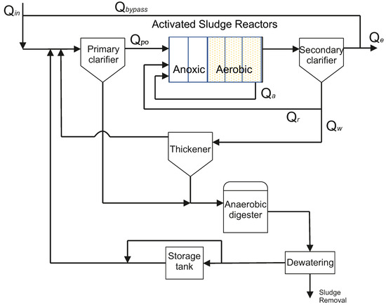
Figure 1.
Benchmark Simulation Model no. 2 (BSM2) plant with notation used for flow rates.
The present work is focused on the secondary treatment and specifically on the biological treatment. The objective of this treatment in WWTPs is to reduce organic matter and nutrients. Phosphorus can be removed biologically or by chemical precipitation, but it is not considered in this model. As mentioned before, the biological treatment of BSM2 is composed of five activated sludge reactors. The first two reactors are anoxic (no oxygen is added), but they contain oxygen in the form of . Here, heterotrophic bacteria degrade organic matter and consume oxygen. As no oxygen is added, the oxygen of is consumed, reducing to nitrogen gas, which is called denitrification process. The next three reactors are aerobic. In these reactors, heterotrophic bacteria also degrade organic matter, but in this case they consume the oxygen added by the blowers. This oxygen is also consumed by autotrophic bacteria, oxidizing to , which is called nitrification process. As there is no at the entrance of the biological treatment, there is an internal recirculation from the last aerobic reactor to the first anoxic reactor. The present work is focused on the flow rate regulation of this internal recirculation.
BSM2 includes 609 days of influent data, including periods of dry, rainy and storm weather and temperature () variations. The last year is evaluated. The average dry weather flow rate is 20,648.36 m/d and the average COD is 592.53 mg/L. The volume of each anoxic tank is 1500 m and that of each aerobic tank 3000 m. The hydraulic retention time of the biological treatment is 14 h.
The pumping energy is calculated as:
where T is the total time, is the external recycle flow rate, is the wastage flow rate from the secondary clarifier, is the underflow rate from the primary clarifier, is the underflow rate from the thickener and is the underflow rate from the dewatering.
The limits established for in the effluent () and in the effluent () are 18 mg/L and 4 mg/L, respectively.
The Activated Sludge Model No. 1 (ASM1) [14] describes the processes of the biological reactors. They define the conversion rates of the different variables of the biological treatment. The design of the proposed fuzzy controller is based on the conversion rates of () and (), which are shown below:
where , , , are four of the eight biological processes defined in ASM1. Specifically, is the aerobic growth of heterotrophs, is the anoxic growth of heterotrophs, is the aerobic growth of autotrophs and is the ammonification of soluble organic nitrogen. They are defined below:
where is the readily biodegradable substrate and is:
where X is the active autotrophic biomass and is:
where S is the soluble biodegradable organic nitrogen and k is:
The general equations for mass balancing are:
- For reactor 1:where Z is any concentration of the process, Z is Z in the first reactor, is Z in the internal recirculation, is Z in the external recirculation, is Z from the primary clarifier, V is the volume, is V in the first reactor, is the overflow of the primary clarifier and is the flow rate in the first tank and it is equal to the sum of Q, Q and Q.
- For reactor 2 to 5:where k is the number of reactor and is equal to
2.2. Operation Strategy Used for Testing
The control strategy applied in [8] is shown in Figure 2a. The of the aerated reactors is controlled by two Model Predictive Controllers (MPC) with feedforward compensation of the flow rate from the primary clarifier. One MPC controls the in the fourth reactor () set-point by manipulating the oxygen transfer coefficient () of the third reactor () and fourth reactor (). The other MPC controls in the fifth reactor () set-point by manipulating of the fifth reactor (). The variation of set-points is a better option than keeping them fixed in terms of effluent quality and operational costs, as shown in ([15]. In this control strategy, a fuzzy controller is applied to manipulate and set-points based on . Finally, another MPC with feedforward compensation manipulates to control in the second reactor () at the set-point of 1 mg/L (_Man_MPC).
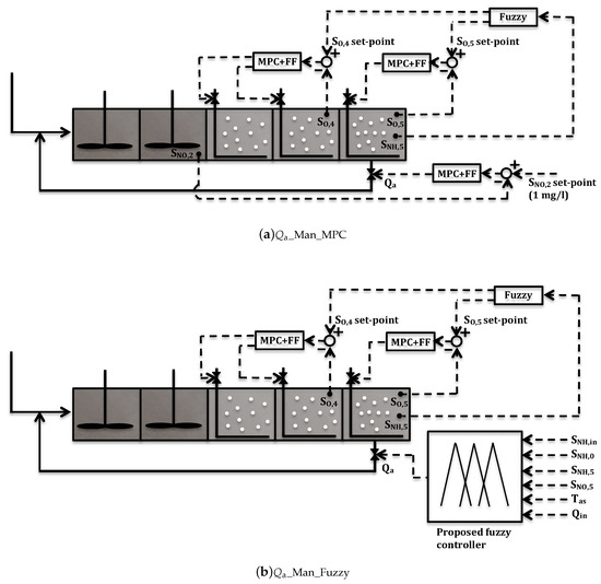
Figure 2.
Operation strategy established in [8], manipulating with control (a) and with the proposed fuzzy controller (b).
3. Fuzzy Controller Design
A fuzzy controller is proposed in this work for manipulation.
Fuzzy logic can be applied as a control technique, relating measured variables (inputs) and manipulated variables (outputs), based on human expertise about the plant to be controlled. Using fuzzy logic, the controller’s input values are converted into words by means of membership functions. These words are used in the established rules that relate the variables of the inputs and outputs of the controller. Subsequently, the words of the outputs are converted into values also by membership functions, which are the resulting values of the manipulated variables.
The principle of fuzzy logic, the design of the proposed fuzzy controller and its application are described below.
3.1. Fuzzy Logic
The fuzzy control is based on the practical knowledge acquired with the operation of the systems. This knowledge is determined by words and expressions and not, as in traditional logic, by numbers and equations. In fact, this does not mean at all that knowledge of the process dynamics is not needed. Good knowledge of the dynamic behaviour of the controlled plant is to be available to the designer. The architecture of a fuzzy controller consists of a fuzzifier, a fuzzy rule base, an inference engine and a defuzzifier ([16,17]).
As the variables are measured in numbers, a fuzzifier is used to convert the inputs into suitable linguistic values, granting them a relative membership degree and not strict. Conversely, a defuzzifier is used to transform the outputs from linguistic values into measured variables. The configuration of a fuzzifier and a defuzzifier implies the selection of the type of membership function, the number of membership functions and the definition of the range of input and output values. The fuzzy rule base is a set of - rules that store the empirical knowledge of the experts about the operation of the process. The fuzzy logic computes the grade of membership of each condition of a rule and aggregates the partial results of each condition using fuzzy set operator. The inference engine combines the results of the different rules to determine the actions to be carried out, and the defuzzifier converts the control actions of the inference engine into numerical variables, determining the final control action that is applied to the plant. There are two different methods to operate these modules: Mamdani ([18]) and Sugeno ([19]). Mamdani system aggregates the area determined by each rule and the output is determined by the centre of gravity of that area. In a Sugeno system the results of the - rules are already numbers determined by numerical functions of the input variables and therefore no deffuzifier is necessary. The output is determined weighting the results given by each rule with the values given by the conditions.
Readers can find further information about fuzzy control in standard references such as [20]. The FIS (FIS: Fuzzy Inference System) Editor from Matlab is used for the implementation of the proposed fuzzy controller.
3.2. Proposed Fuzzy Controller for Manipulation
A fuzzy controller is proposed in this work because the manipulation is based on an exhaustive knowledge of its effects on the different areas of the biological treatment.
The most important relationships between the inputs and output are explained below:
- in the fifth reactor () is always lower than in the influent () due to the nitrification process. On the other side, there is no in the influent, but there is in the fifth reactor (). Therefore, an increase of dilutes at the entrance of the first reactor () and at the entrance of the first reactor () is increased (13) and (14). However, is subsequently reduced in the denitrification process. Consequently, manipulation is related to , and is increased when is higher to dilute , and is decreased when is lower because dilution is not necessary and lower results in operational cost savings and improvements in the nitrification and denitrification processes (12). However, this reduction is always restricted by to have a minimum dilution.
- manipulation influences the Hydraulic Retention Time (HRT), increasing it when is lower. On the other side, during the biological process, substrate is biodegraded by heterotrophic bacteria, and therefore the reduction increases substrate in the biological process. Hence, increases of HRT and substrate improve the denitrification process, reducing (3), (6) and (12). However, HRT increases also improve the nitrification process, which can cause a increase a little later, but it also depends on . Therefore, is decreased when increases to improve the denitrification process, but not excessively so as not to generate too much in the nitrification process. The best option to avoid limit violations is to reduce just at the peak.
- Any rule that increases is always restricted by , since if it increases to near the established limit is reduced to improve the nitrification process and thus oxidize more .The resulting fuzzy controller consist of 30 rules based on the effects on the biological treatment. It has 6 inputs and 1 output. The inputs are , , , , T and influent flow rate () and the output is . Mamdani ([18]) is the method of inference. T has two membership functions: “low” and “high” (Figure 3e) and the rest of inputs have three membership functions: “low”, “medium” and “high” (Figure 3a–d,f). The output has six membership functions: “very_low”, “low”, “medium_low”, “medium”, “high” and “very_high” (Figure 3g).
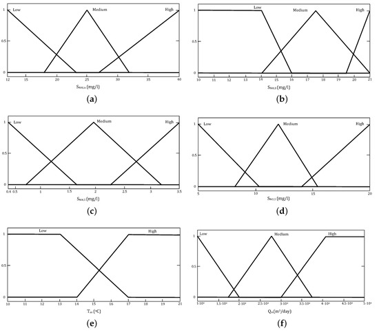
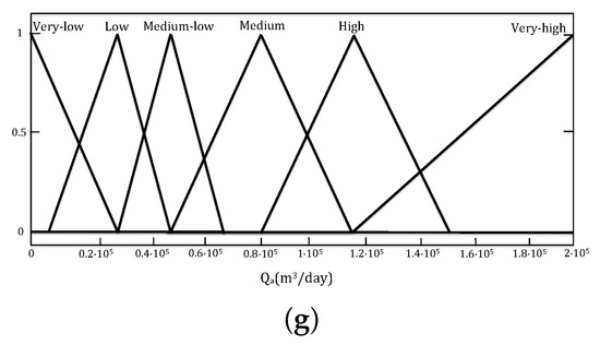 Figure 3. Membership functions of inputs and the output of the proposed fuzzy controller. (a) Membership functions of . (b) Membership functions of . (c) Membership functions of . (d) Membership functions of . (e) Membership functions of . (f) Membership functions of . (g) Membership functions of .
3.3. Application of the Proposed Fuzzy Controller
Figure 2b shows the proposed application of the fuzzy controller for manipulation in the operation strategy of [8] (_Man_Fuzzy). The control in the aerated reactors is kept and only the MPC that controls by manipulating is replaced by the proposed fuzzy controller. In this way, the proposed fuzzy controller for manipulation is tested in an already established and published operation strategy and compared with a usual manipulation based on control. The objective is not only to compare the achieved results, but also to analyse and compare the different effects of variations on pollutants concentrations and costs.
4. Simulation Results and Discussion
In this section, simulation results of the operation strategy applied in [8] with _Man_MPC (Figure 2a) and _Man_Fuzzy (Figure 2b) are compared and discussed, analysing the evolution over time of the most important variables.
Table 1 shows the simulation results of the percentage of time of and limit violations and the pumping energy consumption with _Man_MPC _Man_Fuzzy. Among these results, the reductions of 59.40% in limit violations and 38% in pumping energy by _Man_Fuzzy are remarkable. These improvements do not result in a deterioration of the percentage of time of limit violations, since it is similar with both manipulations and even with a 2.35% improvement with _Man_Fuzzy.

Table 1.
Numerical results with _Man_MPC and _Man_Fuzzy.
As there is no at the entrance of the biological treatment, but there is at the output, the manipulation based on control increases when is lower to increase to the set-point of 1 mg/L.The main disadvantage of the control is that this fact increases pumping energy consumption too much, specially at high , when the nitrification and denitrification processes improve and less dilution is necessary. This can be observed in Figure 4, which shows the results of a week simulation in summer. The difference in values between _Man_MPC and _Man_Fuzzy is very large when and are lower enough than the established limits. In addition, in this specific control technic, MPC achieves a satisfactory tracking, but some abrupt increases, due to its high gain, result in increases that reach values over the established limits in some cases, such as on days 589 and 590.
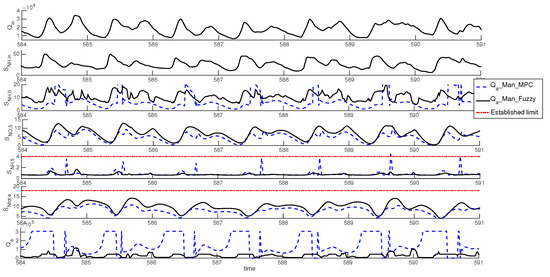
Figure 4.
Time evolution of , , , , , and during one week in summer with _Man_MPC and _Man_Fuzzy.
Figure 5 shows the day 559, in which a high rain event takes place. When it happens, the increase results in a HRT reduction, worsening the nitrification and denitrification processes, and consequently and increase. As a result of this increase, _Man_MPC reduces to try to keep at the set-point of 1 mg/L. Then, there is an important difference between _Man_Fuzzy and _Man_MPC between the times 559.3 and 559.4 since when there is a increase, _Man_Fuzzy increases , but _Man_MPC keeps a low value. This fact results in an important difference in the dilution. When the peak reaches the aerated reactors, detected by the input, _Man_Fuzzy reduces to similar levels of _Man_MPC to improve the nitrification process. As can be observed between the times 559.4 and 559.5, the limit violation is avoided with _Man_Fuzzy but not with _Man_MPC, which is mainly due to the previous dilution. This fact also produces a slight reduction of the peak and therefore of the peak, although the limit violation is not avoided. A greater peak reduction could be achieved if is reduced later, when is higher, but this manipulation would not avoid the limit violation.
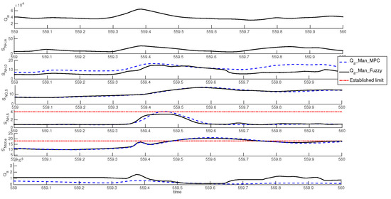
Figure 5.
Time evolution of , , , , , and of day 559 with _Man_MPC and _Man_Fuzzy.
A similar case happens on day 599, as shown in Figure 6. _Man_MPC decreases too much when there is rain event, while _Man_Fuzzy increases when increases, resulting in a significant difference in dilution, specially between the times 599.3 and 599.4. In this case, the limit violation is avoided with _Man_Fuzzy.
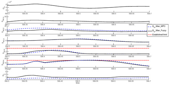
Figure 6.
Time evolution of , , , , , and of day 599 with _Man_MPC and _Man_Fuzzy.
Figure 7 shows a week simulation in winter, when is lower. There is no significant difference in the values between _Man_MPC and _Man_Fuzzy, only in specific short time periods. Therefore, the pumping energy savings of _Man_Fuzzy in comparison with _Man_MPC are mainly achieved with higher . It can be observed that with dry weather and low the variations are similar with both applications. However, the increase with _Man_MPC coincides with a increase, but is due to a decrease caused for a previous decrease, while _Man_Fuzzy increases due specifically to a increase. In the case of an influent with low values during a longer period, applying _Man_MPC could result in a larger and unnecessary increase without coinciding with a increase, as in the similar case of the summer period (Figure 4). On the other hand, the reduction is due to the increase with both manipulations, even though _Man_MPC does not take into account the increase, while _Man_Fuzzy does. This fact explains the similar percentage of time of limit violations with both manipulations and the improvement of limit violations by applying _Man_Fuzzy.
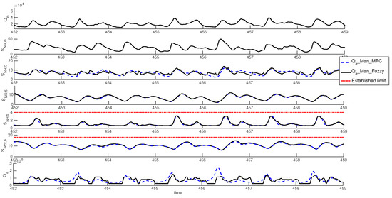
Figure 7.
Time evolution of , , , , , and during one week in winter with _Man_MPC and _Man_Fuzzy.
5. Conclusions
An alternative for manipulation in the biological wastewater treatment by a fuzzy controller has been proposed instead of the usual control. Both manipulations has been tested and compared applying them in an already published operation strategy, obtaining the following conclusions:
- _Man_Fuzzy takes into account values for manipulation, but _Man_MPC is based only on values. This fact added to the abrupt variations with _Man_MPC results in a 59.40% reduction of limit violations with _Man_Fuzzy in comparison with _Man_MPC
- With lower values, the _Man_MPC application increases . This fact takes place specially at higher , when the dilution is less necessary, while _Man_Fuzzy application keeps lower values without risk of violations. As a result, _Man_Fuzzy gets a 38% reduction in pumping energy compared to _Man_MPC.
- Both _Man_MPC and _Man_Fuzzy reduce when increases. Due to this fact, the percentages of time of limit violations are similar with both applications. The 2.35% reduction with _Man_Fuzzy is mainly due to rain events because _Man_MPC keeps very low to reduce , without taking into account the dilution, as _Man_Fuzzy does.
Author Contributions
Conceptualization, I.S., R.V., C.P., and M.B; methodology, I.S.; software, I.S.; validation, I.S., R.V., C.P., and M.B; formal analysis, I.S. and R.V; investigation, I.S.; resources, R.V.; data curation, I.S.; writing–original draft preparation, I.S; writing–review and editing, I.S. and R.V; visualization, I.S., R.V., C.P., and M.B; supervision, R.V., C.P., and M.B.; project administration, R.V.; funding acquisition, R.V. All authors have read and agreed to the published version of the manuscript.
Funding
This research was funded by the Spanish CICYT program under grant DPI-2016-77271-R.
Acknowledgments
Marian Barbu acknowledge the suport of the project “EXPERT”, Contract no. 14PFE/17.10.2018.
Conflicts of Interest
The authors declare no conflict of interest.
Abbreviations
The following abbreviations are used in this manuscript:
| ASM1 | Activated Sludge Model no. 1 |
| 5-day Biological Oxygen Demand (mg/L) | |
| BSM1 | Benchmark Simulation Model no 1 |
| BSM2 | Benchmark Simulation Model no2 |
| Chemical Oxygen Demand (mg/L) | |
| HRT | Hydraulic Retention Time (s) |
| Oxygen transfer coefficient (d) | |
| Oxygen transfer coefficient in tank i (d) | |
| Q | Flow rate (m/d) |
| Internal recycle flow rate (m/d) | |
| Influent flow rate (m/d) | |
| External recycle flow rate (m/d) | |
| Wastage flow rate from the secondary clarifier (m/d) | |
| Underflow rate from the thickener (m/d) | |
| Underflow rate from the dewatering (m/d) | |
| conversion rate of ammonium and ammonia nitrogen concentration in the biological process | |
| conversion rate of nitrate concentration in the biological process | |
| Total nitrogen concentration (mg/L) | |
| Total nitrogen concentration in the effluent (mg/L) | |
| Ammonium and ammonia nitrogen concentration (mg/L) | |
| Ammonium and ammonia nitrogen concentration at the input of the first reactor (mg/L) | |
| Ammonium and ammonia nitrogen concentration at the output of the fifth reactor (mg/L) | |
| Ammonium and ammonia nitrogen concentration in the influent (mg/L) | |
| Ammonium and ammonia nitrogen concentration in the effluent (mg/L) | |
| Nitrate concentration (mg/L) | |
| Nitrate concentration at the input of the first reactor (mg/L) | |
| Nitrate concentration at the output of the second reactor (mg/L) | |
| Nitrate concentration at the output of the fifth reactor (mg/L) | |
| Dissolved oxygen concentration (mg/L) | |
| Dissolved oxygen concentration in tank i (mg/L) | |
| Temperature (C) | |
| Total Suspended Solids (mg/L) | |
| WWTP | Wastewater Treatment Plants |
| Z | any concentration of the process |
| is Z at the output of the reactor i |
References
- Solon, K.; Flores-Alsina, X.; Mbamba, C.K.; Ikumi, D.; Volcke, E.; Vaneeckhaute, C.; Ekama, G.; Vanrolleghem, P.; Batstone, D.J.; Gernaey, K.V.; et al. Plant-wide modelling of phosphorus transformations in wastewater treatment systems: Impacts of control and operational strategies. Water Res. 2017, 113, 97–110. [Google Scholar] [CrossRef] [PubMed]
- de Canete, J.F.; del Saz-Orozco, P.; Gómez-de Gabriel, J.; Baratti, R.; Ruano, A.; Rivas-Blanco, I. Control and soft sensing strategies for a wastewater treatment plant using a neuro-genetic approach. Comput. Chem. Eng. 2021, 144, 107146. [Google Scholar] [CrossRef]
- Santín, I.; Barbu, M.; Pedret, C.; Vilanova, R. Control strategies for nitrous oxide emissions reduction on wastewater treatment plants operation. Water Res. 2017, 125, 466–477. [Google Scholar] [CrossRef] [PubMed]
- Zhang, A.; Yin, X.; Liu, S.; Zeng, J.; Liu, J. Distributed economic model predictive control of wastewater treatment plants. Chem. Eng. Res. Des. 2019, 141, 144–155. [Google Scholar] [CrossRef]
- Revollar, S.; Vega, P.; Vilanova, R.; Francisco, M. Optimal control of wastewater treatment plants using economic-oriented model predictive dynamic strategies. Appl. Sci. 2017, 7, 813. [Google Scholar] [CrossRef]
- Sadeghassadi, M.; Macnab, C.J.; Gopaluni, B.; Westwick, D. Application of neural networks for optimal-setpoint design and MPC control in biological wastewater treatment. Comput. Chem. Eng. 2018, 115, 150–160. [Google Scholar] [CrossRef]
- Qiao, J.F.; Hou, Y.; Zhang, L.; Han, H.G. Adaptive fuzzy neural network control of wastewater treatment process with multiobjective operation. Neurocomputing 2018, 275, 383–393. [Google Scholar] [CrossRef]
- Santín, I.; Pedret, C.; Vilanova, R.; Meneses, M. Advanced decision control system for effluent violations removal in wastewater treatment plants. Control Eng. Pract. 2016, 279, 207–219. [Google Scholar] [CrossRef]
- Alex, J.; Beteau, J.; Copp, J.; Hellinga, C.; Jeppsson, U.; Marsili-Libelli, S.; Pons, M.; Spanjers, H.; Vanhooren, H. Benchmark for evaluating control strategies in wastewater treatment plants. In Proceedings of the Control Conference (ECC), Karlsruhe, Germany, 31 August–3 September 1999; pp. 3746–3751. [Google Scholar]
- Copp, J.B. The COST Simulation Benchmark: Description and Simulator Manual: A Product of COST Action 624 and COST Action 682; Office for Official Publications of the European Union: Luxembourg, 2002. [Google Scholar]
- Gernaey, K.; Jeppsson, U.; Vanrolleghem, P.; Copp, J. Benchmarking of Control Strategies for Wastewater Treatment Plants; Scientific and Technical Report No.23; IWA Publishing: London, UK, 2014. [Google Scholar]
- Jeppsson, U.; Pons, M.N.; Nopens, I.; Alex, J.; Copp, J.; Gernaey, K.; Rosen, C.; Steyer, J.P.; Vanrolleghem, P. Benchmark Simulation Model No 2: General protocol and exploratory case studies. Water Sci. Technol. 2007, 56, 67–78. [Google Scholar] [CrossRef] [PubMed]
- Nopens, I.; Benedetti, L.; Jeppsson, U.; Pons, M.N.; Alex, J.; Copp, J.B.; Gernaey, K.V.; Rosen, C.; Steyer, J.P.; Vanrolleghem, P.A. Benchmark Simulation Model No 2: Finalisation of plant layout and default control strategy. Water Sci. Technol. 2010, 62, 1967–1974. [Google Scholar] [CrossRef] [PubMed]
- Henze, M.; Grady, C.; Gujer, W.; Marais, G.; Matsuo, T. Activated Sludge Model 1; Scientific and Technical Report No.1; IAWQ: London, UK, 1987. [Google Scholar]
- Santín, I.; Pedret, C.; Vilanova, R. Applying variable dissolved oxygen set point in a two level hierarchical control structure to a wastewater treatment process. J. Process Control 2015, 28, 40–55. [Google Scholar] [CrossRef]
- Bai, Y.; Zhuang, H.; Wang, D. Advanced Fuzzy Logic Technologies in Industrial Applications (Advances in Industrial Control); Springer: London, UK, 2006. [Google Scholar]
- Chen, G.; Pham, T.T. Introduction to Fuzzy Sets, Fuzzy Logic, and Fuzzy Control Systems; CRC Press: Boca Raton, FL, USA, 2000. [Google Scholar]
- Mamdani, E. Application of Fuzzy Algorithms for Control of Simple Dynamic Plant. Proc. Inst. Electr. Eng. 1976, 121, 1585–1588. [Google Scholar] [CrossRef]
- Takagi, T.; Sugeno, M. Fuzzy Identification of System and its applications to Modeling and Control. IEEE Trans. Syst. Man, Cybern. 1985, 15, 116–132. [Google Scholar] [CrossRef]
- Klir, G.; Yuan, B. Fuzzy Sets and Fuzzy Logic; Prentice Hall: Upper Saddle River, NJ, USA, 1995; Volume 4. [Google Scholar]
Publisher’s Note: MDPI stays neutral with regard to jurisdictional claims in published maps and institutional affiliations. |
© 2020 by the authors. Licensee MDPI, Basel, Switzerland. This article is an open access article distributed under the terms and conditions of the Creative Commons Attribution (CC BY) license (http://creativecommons.org/licenses/by/4.0/).