CFD Simulation of Forced Recirculating Fired Heated Reboilers

Abstract

An advanced algorithm has been developed in order to analyze the performance of re-boiling process of crude oil flowing inside reboilers tubes. The proposed model is composed from Heptane fire heater and a tube array. The heat flux produced from burner is transferred to the crude oil flowing inside the tube. The computational model is composed of two phases—Simulation of fire by using Fire Dynamics Simulator software (FDS) version 5.0 and then a nucleate boiling computation of the crude oil. FDS code is formulated based on CFD (Computational Fluid Dynamics) of fire heater. The thermo-physical properties (such as: thermal conductivity, heat capacity, surface tension, viscosity) of the crude oil were estimated by using empirical correlations. The thermal heat transfer to evaporating two-phase crude oil mixture occur by bubble generation at the wall (nucleate boiling) has been calculated by using Chen correlation. It has been assumed that the overall convective heat transfer coefficient is composed from the nucleate boiling convective coefficient and the forced turbulent convective coefficient. The former is calculated by Forster Zuber empirical equation. The latter is computed from the Dittus-Boelter relationship. In order to validate the nucleate boiling heat transfer coefficient, a comparison has been performed to nucleate boiling convective coefficient obtained by Mostinski equation. The relative error between the nucleate boiling convective heat-transfer coefficients is 10.5%. The FDS numerical solution has been carried out by using Large Eddy Simulation (LES) method. This work has been further extended to include also the structural integrity aspects of the reboiler metal pipe by using COMSOL Multiphysics software. It was found out, that the calculated stress is less than the ultimate tensile strength of the AISI 310 Steel alloy.

1. Introduction

Several works have been written about crude oil boiling. Sciance [1] has conducted experiments on nucleate and film saturated pool boiling for several hydrocarbons, such as: methane, ethane at twelve reduced pressures (the ratio between the pressure and the critical pressure). These experiments have been performed between 0.02 (atmospheric pressure) and 0.9 (close to critical pressure). He has been obtained complete burnout flux (critical heat flux) vs. reduced pressure curves for each substance. The Critical Heat Flux (CHF) equation derived by Noyes [2] describes these experimental data with reasonable accuracy over the entire pressure range. Zhu [3] has applied Wall-Resolved Large Eddy Simulation (WRLES) in order to study non-reacting and reacting flows in both smooth and ribbed tubes, to show the impact of the ribs on turbulence and chemistry. The CFD (Computational Fluid Dynamics) simulations were performed with the AVBP code. This code is a parallel CFD code that solves the 3D compressible momentum equations for turbulent flows, with coupling of reduced chemistry scheme of ethane and butane cracking for reacting cases.

This work includes analysis of Fire heater and Crude boiling process. The computational process algorithm is composed of four components. Fire Dynamics Simulator (FDS) outputs a file which contains the Heptane flame simulation data, STNAJAN software which evaluates the thermo-physical properties of the burned gaseous mixture (thermal conductivity, kinematic viscosity etc.), COMSOL Multi-physics transient axi-symmetrical model which performs Heat transfer and structural analyses, and the main program which calculates the nucleate boiling convective coefficient and the external flow convective coefficient of the gaseous mixture produced from Heptane burning. It also includes the radiation heat flux emitted by the soot particles. The COMSOL Multiphysics software have been loaded with the radiative and convective heat fluxes emitted by gaseous and soot mixture.

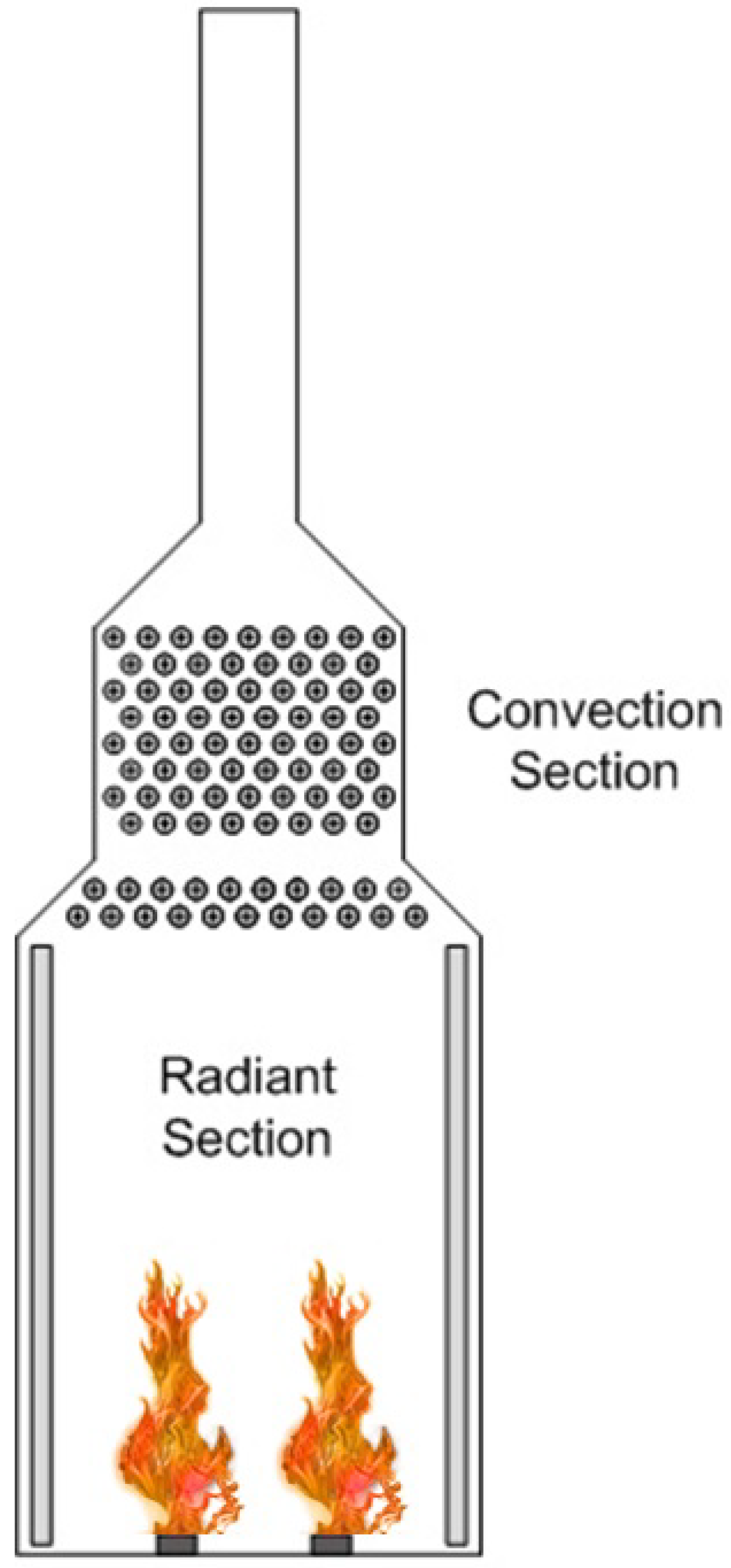
1.1. Fired Heated Furnaces

In order to utilize the heat released by combustion, it must be set free in an enclosed space made of brick or other resistant material, known furnace. Furnaces may in general be divided into two types [4]. In the first type, the combustion is transferred by direct contact to the hot gaseous mixture produced by the combustion. In the second type, the heat transmitted to the crude oil by utilizing a heat exchanger. The combustion exhausts gases products, are completely separated from the crude oil tubes. The former type of furnace has the great advantage of cheaper construction and lower cost of maintenance and operation. It is adapted to maintain a higher temperature. The disadvantages are that the tubes may be contaminated with soot particles, smoke, or other products. The steel may also be exposed to oxidizing species such as steam, carbon monoxide, or carbon dioxide. If fuel is contaminated with Sulphur, these tubes may be exposed to Sulphur acid. On the other hand, the second type—heat exchanger has the obvious advantage of filtration of soot or smoke, more uniform control of the temperature and the chemical conditions of the existing combustion products. The disadvantages embedded in second type are heat losses and pressure losses inside the tube pipe. The maintenance is more expensive. The steel tube may be damaged by each of following mechanisms [5]: Cavitation damage, corrosion fatigue, high temperature corrosion, pitting corrosion, stress corrosion cracking, thermal creep, and fouling (water boiling surfaces usually acquire deposits, often referred to as “crud”).

In the framework of this study, an analysis has been performed of the first type device. It should be noted that the algorithm described here is robust and can be adapted to simulate the second type furnace (The convective heat transfer coefficient obtained in Section 2.6 can be adapted to handle with steam or other high temperature heat carriers such as DOWTHERM A [6,7,8,9]). It is assumed that the thermal energy released by the combustion of fuel is transmitted to crude oil flowing inside the tubes. The furnace shown in Figure 1 is composed of three major components: the radiant section, the convection section, and the stack [10]. It is fueled by Heptane liquid fuel. The crude oil liquid, flowing inside the tubes, absorbs the heat mostly by radiative and convective heat transfer from the flue gases [11].

The height of the furnace is 8 m above the ground [11]. Initially, the flame velocity is normally high enough to produce large turbulent eddy motion. Friction occurs between the boundary of the flame and its surroundings, causing the surrounding air to be locally accelerated to the flame velocity. The accelerated air is then mixed with the flame and expanding it. This process is called entrainment [11]. The mixing is accomplished by turbulent eddy motion [12]. At the end of this process, the velocity of the flame and surroundings become homogenous. The analysis of such flames is based on mixing process only. In industrial furnaces, rapid fuel combustion occurs. The combustion of flame fuel in industrial furnaces as well as engines of various types is rapid process [12]. The heat released from fuel burning and carried by exhaust gaseous mixture and soot particles is transferred to reboiler tubes walls in by three main modes: forced and natural convection, thermal radiation, and conduction [13,14].

1.2. Reboiler

Reboilers are applied to provide the vapor flux to feed the bottom tray of the distillation column. The liquid exiting from the bottom of the column is partially vaporized in heated fired furnace. It is assumed that the heating medium is flue gaseous mixture produced by Heptane burning. There are three principal types of reboilers utilized in the distillation columns [15]:

(1)

Forced Recirculation Reboiler

(2)

Thermosiphon Natural Circulation Reboiler

(3)

Kettle type

(4)

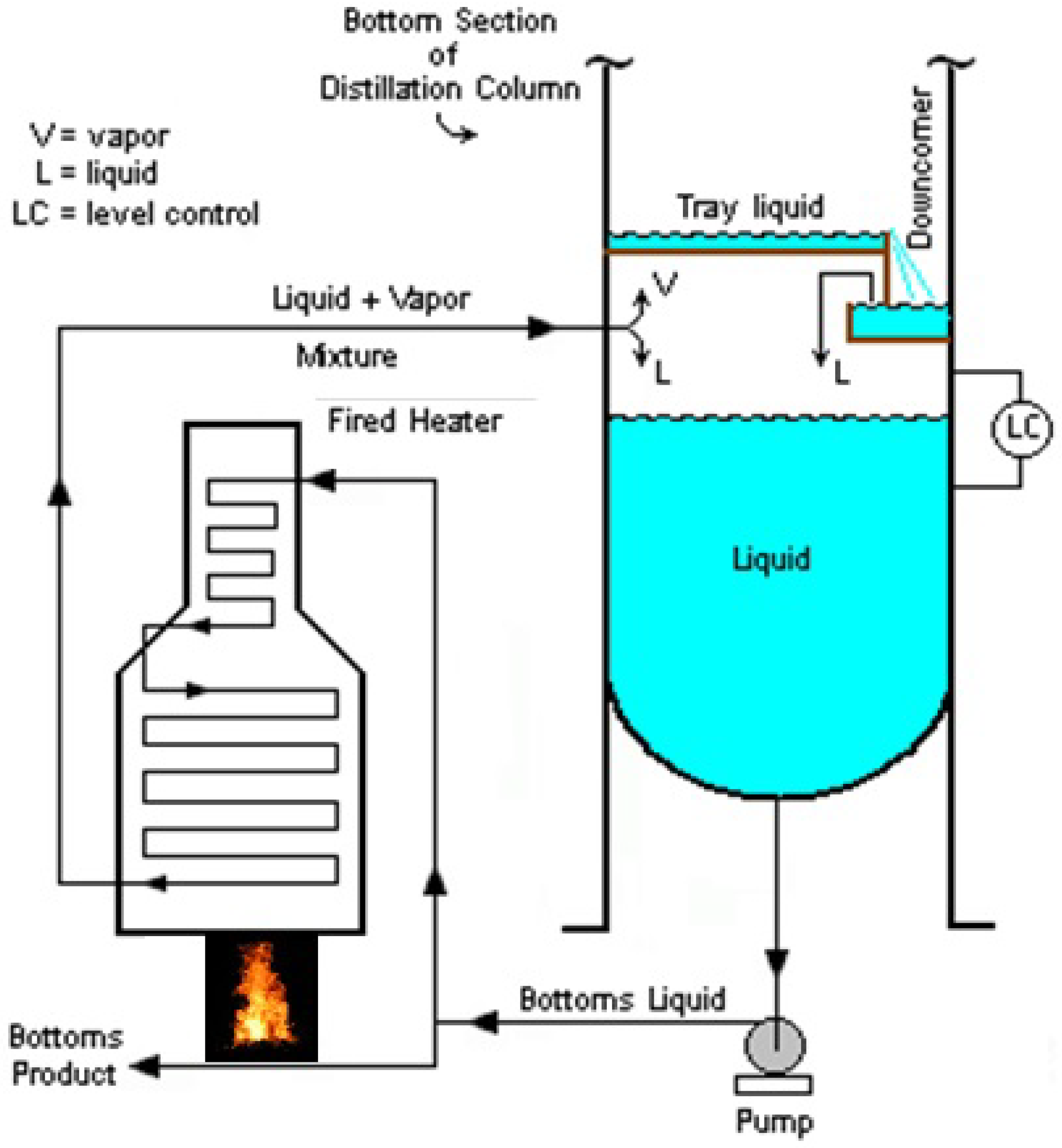
Forced Recirculating Fired Heated Reboiler (see Figure 2)

Distillation bottom crude oil liquids are often mixtures having substantial different boiling ranges. Thermo-physical properties of the liquid and vapor exhibit large variations throughout the reboiler. Thermodynamic calculations are required to determine the phase compositions and other properties within the reboiler. The next sections give theoretical fundamentals of the vapor-liquid equilibrium, the boiling regimes, mechanism of the nucleate boiling, and the thermo-physical properties evaluation of the crude oil.

1.3. Two-Phase Flow Heat Transfer Inside the Reboiler

The Definition of Flow Regimes

The main characterizing feature of two-phase flows is the fact that an interface exists between the two phases and, in gas and liquid flows, this interface takes a wide variety of forms. In general the surface tension effects tend to create curved interfaces leading to spherical shapes (e.g., droplets or bubbles). As the discontinuities in the continuous phase are increased, the departure from a spherical shape is also increased. Thus, small droplets tend to be spherical whereas bigger ones are often deformed in the gas flow, and likewise the bubble. For vertical flows, the regimes to be defined here are illustrated in Figure 3.

The various regimes are defined as follows [16]:

(1)

Bubble flow—the bubbles dispersed in a continuum of liquid

(2)

Slug or plug flow—as the concentration of bubbles increases, the bubble coalescence occurs and, progressively, the bubble diameter approaches that of the tube. Once this occurs, the bubble is bullet-shaped.

(3)

Churn Flow—as the gas flow is increased and the velocity of the slug-flow bubbles increased, the break-down of these bubbles occurs, leading to unstable regime. For narrow-bore tubes the oscillations may not occur and a smoother transition between the slug and annular flow may be observed.

(4)

Annular flow—in this regime, the liquid flows on the wall of the tubes as a film and the gas phase flows in the center. Some of the liquid phase is entrained as small droplets in the gas core.

(5)

Wispy annular flow—for high mass velocity flows, the droplet concentration in the gas core of annular flow increases and, ultimately droplet coalescence occurs, leading to streaks or “wisps” of liquid occurring in the gas core.

2. Materials and Methods

2.1. Calculation of Nucleate Boiling Convective Coefficient

When heat is gradually transferred to the crude oil, several processes are taking place. As the temperature of the crude oil exceeds the boiling point, it begins to evaporate.

At first, individual bubbles form at the heating surface (saturation state). When they reach a particular diameter, they are breaking away and as a result, there is intensive agitation of the boundary layer and the whole mass of boiling liquid. As the heat flux increases the number of crude oil bubbles formed at the heating surface increases. This leads to a further increase in turbulence, and a rapid rise in the heat transfer coefficient. The boiling regime occurring during bubble generation in the vicinity of the tube wall surface is called “nucleate boiling”.

In this boiling regime, high values of convective heat transfer are obtained with relatively small temperature gradient. Nucleate boiling is intensified as the wall temperature increases but is suppressed as the fluid velocity increases. As the forced convection component increases, the nucleate boiling component decreases (by suppression). The most widely used empirical equation which combines these two processes has been derived by Chen [17]. It takes the form:

$$h_B=h_{FC}+h_{NB}=h_{FC}+S_{NB}{h}_{FZ}$$

(1)

Here $h_B$ denotes the two-phase convective boiling heat transfer coefficient (W/m² K), $h_{FC}$ denotes the forced convective boiling heat transfer coefficient (W/m² K), and $h_{NB}$ is the nucleate boing convective. $h_{FZ}$ denotes the nucleate boiling convective heat transfer coefficient (W/m² K). It is calculated by using the Forster-Zuber empirical equation (see Equation (7)). This correlation gives good results when used in Equation (1). $S_{NB}$ is the suppression factor which account for the reduction in the coefficient due to the suppression of nucleation sites. It is related to the total Reynolds number as shown in Figure 4 [18].

The suppression factor S_NB is a function of a two-phase Reynolds number, Re_TP:

$$S_{NB}=\frac{1}{1+2.53\cdot {10}^{-6}{\mathrm{Re}}_{TP}^{1.17}}$$

(2)

The two-phase Reynolds number is calculated according to the following equation:

$${\mathrm{Re}}_{TP}={\mathrm{Re}}_L{F}_c^{1.25}$$

(3)

Here ${\mathrm{Re}}_L$ denotes the liquid phase Reynolds number. It is defined by:

$${\mathrm{Re}}_L=\frac{\dot{m}\left(1-x_G\right)D}{{\mu }_L}$$

(4)

$F_c$ denotes the Reynolds number factor. This factor accounts for the enhanced flow and turbulence due to the presence of vapor. This term can be approximated by [18]:

$$\begin{array}{l}{F}_c=1\mathrm{for}1/X_{tt}<0.1\\ F_c=2.35{\left(0.213+\frac{1}{X_{tt}}\right)}^{0.736}\mathrm{for}1/X_{tt}>0.1\end{array}$$

(5)

$F_c$ is graphically presented in Figure 5 [18].

$X_{tt}$ denotes the Martinelli parameter. This term is calculated by the following equation [18]:

$$\frac{1}{X_{tt}}={\left(\frac{x}{1-x}\right)}^{0.9}{\left(\frac{{\rho }_L}{{\rho }_G}\right)}^{0.5}{\left(\frac{{\mu }_G}{{\mu }_L}\right)}^{0.1}$$

(6)

The correlation of Forster and Zuber (1955) for the nucleate boiling coefficient has the form [19]:

$$h_{FZ}=0.00122\frac{\Delta T_{sat}^{0.24}\Delta p_{sat}^{0.75}{c}_{pL}^{0.45}{\rho }_L^{0.45}{k}_L^{0.79}}{{\sigma }^{0.5}\Delta h_{fg}^{0.24}{\mu }_L^{0.29}{\rho }_G^{0.24}}$$

(7)

where $\Delta T_{sat}$ is the wall superheat (K). It is the wall temperature minus saturation temperature. $\Delta p_{sat}$ is the difference in saturation pressure (N/m²) corresponding to the temperature difference $\Delta T_{sat}$. $k_L$ is the thermal conductivity of the liquid (W/m K). $c_{pL}$ is the heat capacity of the liquid phase (J/kg K). ${\rho }_L$ is the density of the liquid phase (kg/m³). ${\rho }_G$ is the density of the vapor phase (kg/m³). ${\mu }_L$ is the viscosity of the liquid phase (kg/m sec). $\sigma$ is the surface tension (N/m). $\Delta h_{fg}$ is the enthalpy of vaporization (J/kg). The forced convective coefficient is derived from the Dittus-Boelter relationship [18]:

$$h_{FC}=0.023{\left[\frac{G\left(1-x\right)D_e}{{\mu }_L}\right]}^{0.8}{\left({\mathrm{Pr}}_L\right)}^{0.4}\frac{k_L}{D_e}F\left(X_{tt}\right)$$

(8)

The nucleate boiling convective coefficient h_NB is related to the convective coefficient calculated for the mixture properties (h_NBM) as follows [15]:

$$h_{NB}=h_{NBM}{F}^{\prime }$$

(9)

where

$$F^{\prime }=\frac{1}{1+A_s\left|y-x\right|}$$

(10)

y denotes the vapor mole fraction of the lighter component equilibrium with the liquid mole fraction of the component x (see Figure 6). The mole fractions x and y can be obtained by Raoult’s rule. This rule states that the partial pressure of a component over a solution is the product of the vapor pressure of that component and the mole fraction of this component [20]. The parameter A_s is calculated by the following equation:

$$A_s=A_0\left(0.88+0.12p\right)$$

(11)

Here p denotes the system pressure in bars. Ao denotes a constant which depends on the binary system. Stephan and Körner give a table for some combinations. They recommend a value of this term should be 1.5 if no other information is available. This method for binary mixtures has been extended to multicomponent mixtures by Stephan and Preusser [21].

The crude oil refinery is composed of several unit operations components, such as: reboilers, heat exchanger, and pumps. Analysis and design of the performance of these components require knowledge of the thermodynamic and physical properties of the crude oil fluids [22]. As described in the previous section designing a reboiler requires knowledge of thermodynamic and thermo-physical properties crude oil. It will be shown later that these are: boiling temperature, pressure, heat capacity, thermal conductivity, diffusivity, and density. Heat exchanger design depends on enthalpies, thermal conductivities, and viscosity of the flowing streams (the crude oil and the steam).

2.2. Estimation of the Thermo-Physical Properties of the Crude Oil

Due to the complexity of the composition crude oils, it is not possible to measure or calculate accurately all of these properties [22]. Furthermore, calculation methods developed for pure hydrocarbons are not always applicable. Over the years, the petroleum refining engineers have developed empirical correlations in order to estimate the properties of crude oil fraction by measuring properties such as specific gravity (SG) and normal boiling point (NBP). Another important term connected with SG is called API gravity. This term is a measure of the relative density of a crude oil liquid and the density of water (i.e., how heavy or light a crude oil liquid is compared to water) [23]. These correlations require minimum input data, and are usually presented in graphical form. These quantities are described in the following section.

In order to calculate the nucleate boiling heat flux, it is essential to estimate the thermo-physical properties of the Crude oil. These properties are described in this section. The thermal conductivity of the crude oil as a function of the temperature is shown in Figure 7 [24].

The density of liquid crude oil is shown in Figure 8.

The viscosity of liquid crude oil is shown in Figure 9.

The latent heat of the crude oil is shown In Figure 10 [25].

The surface tension of the crude oil at three different temperatures: 15.56 °C, 37.78 °C, and 54.44 °C as a function of API (see Figure 11) [26].

It can be seen from this Figure that the surface tension decreases with the API and the temperature. The viscosity of vapor crude oil is shown in Figure 12.

Riazi and Al-Sahhaf [27] evaluated different crude oil properties such as the boiling point, density, refractive index, critical temperature, pressure, and density as a function of the molecular weight by using the following general equation:

$$\theta ={\theta }_{\infty }-\exp \left(a-b{M}^c\right)$$

(12)

Here $\theta$ can be any one of the properties mentioned above. M is the molecular weight and ${\theta }_{\infty }$ is the limiting value for any property as $M\to \infty$. This empirical equation can be applied in order to calculate the following properties. $T_b$ is the mean average boiling point in K, SG is the specific gravity and $p_c$ is the critical pressure in bar. The constants a, b, and c for each property are given in

Table 1. Constants for the Riazi–Al-Sahhaf equation [22,27].

$\mathsf{\Theta }$	${\mathit{\theta }}_{\mathit{\infty }}$	a	b	c
$T_b$	1080	6.97996	0.01964	0.67
SG	1.07	3.56073	2.93886	0.1
$-p_c$	0	6.34492	0.72390	0.3

[22,27].

2.3. Fire Dynamic Simulation (FDS) Modeling of the Fired Heater

The FDS has been developed at the National Institutes of Standards and Technology (NIST) [28,29]. It solves simultaneously the classical conservation equations, which includes the momentum, energy, mass species equations and thermodynamics-based state equation of a perfect gas. The chemical combustion reaction data are taken from a library of different fuel sources. By solving these equations, it calculates the velocity, pressure by solving the momentum equation), temperature (by solving the Energy equation), density (by solving the Equation of state), and chemical composition (by solving the Diffusion equation) within each numerical grid cell as a function of time. It is capable to calculate the heat flux. FDS is composed of three major components:

Hydrodynamic Model—it is formulated based on of fire-driven fluid flow (i.e., natural convection). The numerical solution is carried out using Large Eddy Simulation (LES). This technique is applied for relatively low speeds (or low Reynolds number).

Combustion Model—two types of combustion models are employed in FDS software. The first (regarded as the default) employs the mixture fraction, a quantity representing the fuel and the products of combustion. The second model makes use of the specified Arrhenius reaction parameters for individual gas species. The mass fractions of all of the major reactants and products can be calculated from the mixture fraction by using means of “state relations”, empirical correlations obtained by a combination of simplified analysis and measurements [30].

Radiation Transport—radiative heat transfer is obtained by solving of the radiation transport equation (RTE) for a non-scattering gray gas. In a several number of cases, a wide band model can be applied in place of the gray gas model. A Finite Volume Method (FVM) technique is applied in FDS software in order to solve this equation [29].

The postprocessor of this software is named “smoke-view”. As we shall see in Section 3, it is capable to perform post-processing images of the temperature, velocity, and soot fields. This code has been employed in this algorithm in order to simulate the Heptane combustion performance.

2.4. Governing Transport Equations of FDS Software

The following subsections describe the conservation momentum, mass (continuity), diffusion, and energy transport equations for the Newtonian fluid.

2.4.1. Mass and Species Transport Equations

Mass conservation is expressed as a function of the density, $\rho$ [28]:

$$\frac{\partial \rho }{\partial t}+\nabla \cdot \rho u={\dot{m}}_b^{‴}$$

(13)

where $\rho$ represents the density of the fluid [kg/m³], and u is the velocity field [m/s]. This equation is expressed as a function of each gaseous species, $Y_{\alpha }$:

$$\frac{\partial }{\partial t}\left(\rho Y_{\alpha }\right)+\nabla \cdot \rho Y_{\alpha }u=\nabla \cdot \rho D_{\alpha }\nabla Y_{\alpha }+{\dot{m}}_{\alpha }^{‴}+{\dot{m}}_{b,\alpha }^{‴}$$

(14)

where $D_{\alpha }$ represents the diffusion coefficient of $\alpha$ component of the mixture [m²/s].

2.4.2. Momentum Transport Equation

The momentum equation is described in the following equation [28]:

$$\frac{\partial }{\partial t}\left(\rho u\right)+\nabla \cdot \rho uu+\nabla p=\rho g+f_b+\nabla \cdot {\tau }_{ij}$$

(15)

Here f_b is the force term (gravity force) [Pa/m]. ${\tau }_{ij}$ is the stress tensor, [Pa]. This term is defined as [28]:

$${\tau }_{ij}=\mu \left(2S_{ij}-\frac{2}{3}{\delta }_{ij}\left(\nabla \cdot u\right)\right);{\delta }_{ij}=\{\begin{array}{l}1i=j\\ 0i\ne j\end{array};S_{ij}=\frac{1}{2}\left(\frac{\partial u_i}{\partial x_j}+\frac{\partial u_j}{\partial x_i}\right)i,j=1,2,3$$

(16)

The term S_ij represents the symmetric rate of strain tensor. μ denotes the dynamic viscosity of the fluid. In this work the Heptane fire heater simulation has been carried out by applying LES method, in which the large-scale eddies are calculated directly, and the subgrid-scale dissipative processes are modeled. FDS uses LES in most fire simulation applications. The following subsection contains a description of how the transport dissipative terms are modeled in FDS software.

2.4.3. Large Eddy Simulation (LES) Turbulence Method

Large Eddy Simulation (LES) is applied in FDS software in order to model the dissipative terms (such as: viscosity, thermal conductivity, and material diffusivity) which occur at length scales smaller than those that are explicitly resolved on the numerical computational grid cell. They are replaced by surrogate expressions that “model” their impact on the approximate form of the governing equations (It means that these properties cannot be applied directly in most practical simulations). The dissipation rate, $\epsilon$, [Pa/s] is the rate at which kinetic energy is converted to thermal energy by the viscosity of the gaseous mixture [28]:

$$\begin{array}{l}\epsilon ={\tau }_{ij}\cdot \nabla u=\mu \left(2S_{ij}{S}_{ij}-\frac{2}{3}{\left(\nabla \cdot u\right)}^2\right)=\mu [2{\left(\frac{\partial u}{\partial x}\right)}^2+2{\left(\frac{\partial v}{\partial y}\right)}^2+2{\left(\frac{\partial w}{\partial z}\right)}^2+\\ {\left(\frac{\partial v}{\partial x}+\frac{\partial u}{\partial y}\right)}^2+{\left(\frac{\partial w}{\partial y}+\frac{\partial v}{\partial z}\right)}^2+{\left(\frac{\partial u}{\partial z}+\frac{\partial w}{\partial x}\right)}^2-\frac{2}{3}{\left(\frac{\partial u}{\partial x}+\frac{\partial v}{\partial y}+\frac{\partial w}{\partial z}\right)}^2]\end{array}$$

(17)

The viscosity μ is computed according to the following equation

$${\mu }_{LES}=\rho {\left(C_s\Delta \right)}^2{\left(2{\overline{S}}_{ij}:{\overline{S}}_{ij}-\frac{2}{3}{\left(\nabla \cdot \overline{u}\right)}^2\right)}^{\frac{1}{2}}$$

(18)

Here Δ is a length on the order of the size of a grid cell and C_s represents the empirical constant. The bar above the quantities appearing in Equation (18) represents resolved values. They are calculated from the numerical solution sampled on a coarse grid cell (relative to Direct Numerical Simulation—DNS). The other diffusive parameters such as: material diffusivity and thermal conductivity are functions of the turbulent viscosity. They are calculated by using the following equations [28]:

$$k_{LES}=\frac{{\mu }_{LES}{c}_p}{P{r}_t};\hspace{1em}{\left(\rho \mathrm{D}\right)}_{t,LES}=\frac{{\mu }_{LES}}{S{c}_t}$$

(19)

It is assumed that the two terms, turbulent Schmidt number $S{c}_t$ (defined as the ratio of momentum diffusivity to mass diffusivity) and turbulent Prandtl number $P{r}_t$ (defined as the ratio of momentum diffusivity to thermal diffusivity), are constant for a given scenario. The model for the viscosity, ${\mu }_{LES}$, serves two roles: first, it has the appropriate mathematical form to describe the dissipation of kinetic energy from the flow. Second, it provides a stabilizing effect in the numerical algorithm, damping out numerical instabilities as they arise in the flow field, especially where vorticity is generated.

2.4.4. Energy Transport Equation

The energy transport equation is described as a function of the sensible enthalpy, $h_s$ [J/kg] [28]:

$$\frac{\partial }{\partial t}\left(\rho h_s\right)+\nabla \cdot \left(\rho h_{s}u\right)=\frac{Dp}{Dt}+{\dot{q}}^{‴}-{{\dot{q}}^{‴}}_b-\nabla \cdot {\dot{q}}^{″}+\epsilon$$

(20)

This term depends on the temperature (according to the ideal law assumption) [28]:

$$h_s={\displaystyle \sum _{\alpha }{Y}_{\alpha }{h}_{s,\alpha }}$$

(21)

The sensible heat of each component in the gaseous mixture is calculated by applying Equation (22) [28]:

$$h_{s,\alpha }\left(T\right)={\displaystyle \underset{T_0}{\overset{T}{\int }}{c}_{p,\alpha }\left(T^{\prime }\right)d{T}^{\prime }}$$

(22)

Here ${\dot{q}}^{‴}$ is the volumetric heat release rate produced by the Heptane combustion [W/m³], ${\dot{q}}_b^{‴}$ is the energy transferred to the evaporating Heptane liquid [W/m³] and ${\dot{q}}^{″}$ is the conductive and radiative heat fluxes [W/m²] [28]:

$${\dot{q}}^{″}=k\nabla T-{\displaystyle \sum _{\alpha }{h}_{s,\alpha }\rho D_{\alpha }\nabla Y_{\alpha }+q_r^{″}}$$

(23)

2.4.5. Equation of State

The pressure is computed by applying the ideal gas equation of state [28]:

$$p=\frac{\rho \overline{R}T}{\overline{W}}$$

(24)

where T is the temperature in [K], $\overline{W}$ is the molecular mass of the gaseous mixture in [J/mole], $\overline{R}$ is the gas constant, and p is the pressure in [Pa].

2.4.6. Fire Dynamics Simulation (FDS) Modeling of the Heptane Burner

The geometric model of the Heptane burner is shown in Figure 13.

The height of the burner model is 2.4 m. It should be noted that most tube failures in fired heaters are caused by high tube metal temperatures (TMTs). Flame impingement on the tube external surface caused by long flames results in higher tube metal temperatures and coking that affect the performance of the heater and decrease the strength of the tubes (such as thermal creep) [31]. The length and the width of the burner are 1.2 m. The mesh size of the burner is: 27,468 cells. At the bottom of the burner, liquid Heptane is injected and ignited. The green points indicate the positions of the thermocouples and the soot particle sensors. The heat of combustion of Heptane is 44,600 (kJ/kg) [32]. The thermal conductivity of the liquid Heptane is 0.14 (W/(m·K)) [33]. Its specific heat is 2.24 (kJ/(kg·K)) [34], and its density is 679.5 (kg/m³) [35]. The soot yield of Heptane is: 0.037 [36].

Initial condition—it is assumed that the initial temperature, the component concentration in the air and pressure are:

$$T_0={20}^{o}C;c_{O_2,0}=0.21;c_{N_2,0}=0.79;c_{i,0}=0;p=101,325\mathrm{Pa}$$

Boundary Condition—it is assumed that all four boundaries are opened to the atmosphere.

$$T={20}^{o}C;c_{O_2}=0.21;c_{N_2}=0.79;c_{i,0}=0;p=101,325\mathrm{Pa}$$

2.5. Turbulent Flow through Reboiler tube bundle

Schematics of the reboiler tube bundle system are shown at Figure 14. The hot gas mixture enters from above. The crude oil flows through the pipe and enters from the side. The tubes are assumed to be made of Stainless Steel.

The arrows in Figure 14 indicate the flows directions of the crude oil and hot combustion products. The corresponding 2D domain appears in Figure 15.

The arrows presented in Figure 16 indicate the flow direction the Heptane combustion products.

2.6. Convective Heat Transfer across Banks of Tubes

This section deals with heat transfer to bundle of tubes inside the reboiler. For flue gaseous mixture flowing across tube bundles composed of 10 or more rows, Grimison [37] has obtained a correlation of the form:

$$N{u}_D=1.13C_1{\mathrm{Re}}_{D,\max }^m{\mathrm{Pr}}^{1/3}$$

(25)

where $N{u}_D$ is the Nusselt number. It is defined in the following equation:

$$N{u}_D\equiv \frac{hD}{k}$$

(26)

where h is the convection coefficient in [W/(m²·K)], D is the tube diameter in [m], and k is the thermal conductivity of the gaseous mixture in [W/(m·K)]. Pr is the Prandtl number. It is the ratio between the kinematic viscosity, ν [m²/sec] to the thermal diffusivity, α [m²/sec]. It is assumed that longitudinal spacing between tube centers (S_L) is equal to the transverse spacing between tube centers (S_T). The spacing between the tube centers is equal to twice of the tube diameter. Thus:

$$S_T=S_L=2D$$

(27)

According to Incropera et al. [38], the values of the constants C₁ and m are:

$$C_1=0.482,m=0.556$$

(28)

${\mathrm{Re}}_{D,\max }$ denotes the Reynolds number of the external flow. This term is defined in Equation (29):

$${\mathrm{Re}}_{D,\max }\equiv \frac{V_{\max }D}{\nu }$$

(29)

D denotes the tube diameter in [m] and $\nu$ denotes the kinematic viscosity of the flue gaseous mixture. $V_{\max }$ [m/sec] is the maximal velocity. It is calculated from Equation (30):

$$V_{\max }=\frac{S_T}{S_T-D}V$$

(30)

The value of the flue gas velocity, V, is obtained from FDS calculation of flame. The required transport properties of the flue gaseous mixture were calculated by using STANJAN software [39]. The required mole fraction of the products species of the oxidation reaction were calculated from the following reaction:

$$C_7{H}_{16}+11O_2\Rightarrow 7C{O}_2+8H_{2}O$$

(31)

The flame temperature of the Heptane flame was obtained by using the FDS software. The transport thermo-physical properties are listed in

Table 2. Transport thermo-physical properties of flue gaseous mixture [38].

Symbol	Value
$\rho (density)$	0.335 [kg/m3]
$\alpha (thermaldiffusivity)$	1.90 × 10−4 (m2/s)
$\nu (kinematicviscosity)$	1.28 × 10−4 (m2/s)
$k(thermalconductivity)$	0.102 [w/(m·K)]

.

2.7. Calcaulation of the Radiative Heat Flux Emitted by the Mixture Flue Gaseous and the Soot Particles

The of radiative heat transfer within the fire heater enclosure are composed of two components: the high temperature burned gaseous mixture and the soot particles within the Heptane flame [13]. The burned gaseous mixture is composed mainly of the carbon dioxide and water vapor. They are not grey but emit and absorb radiation only in the discrete bands in the spectrum and therefore, have mean absorption coefficients which vary with gas temperature and the radiation source. The emissivity of the gaseous mixture can be obtained by adding the absorption coefficient for the gas and soot in each spectral line. The overall emissivity of the gas-soot mixture is given in the following equation [40]:

$${\epsilon }_{\mathrm{m}}={\displaystyle \sum _n{a}_{g,n}}\left(T\right)\left(1-e^{-K_{n}L}\right)$$

(32)

where:

$$K_n=k_{s,n}{C}_{soot}+k_{g,n}\left(p_{C{O}_2}+p_{H_{2}O}\right)$$

(33)

The weighting factors and absorption coefficients for a three-term equation have been evaluated for the case of a mixture of the products of oil combustion. $C_{soot}$ is the soot concentration. It is obtained by applying FDS software (see Figure 23). The weighting factors, $a_{g,n}$ varies linearly with temperature, such that:

$$a_{g,n}\left(T\right)=b_{1,n}+b_{2,n}T$$

(34)

The values of the coefficients $b_{1,n},b_{2,n},k_{s,n},k_{g,n}$ obtained for the mixture emissivity are given in

Table 3. Spectral constants in the mixture of gas and soot emissivity equation [39].

n	${\mathit{b}}_{1,\mathit{n}}$	${\mathit{b}}_{2,\mathit{n}}\left[1/\mathbf{K}\right]$	${\mathit{k}}_{\mathit{g},\mathit{n}}{[\mathbf{m}\times \mathbf{atm}]}^{-1}$	${\mathit{k}}_{\mathit{s},\mathit{n}}\left[{\mathbf{m}}^2/\mathbf{kg}\right]$
1	0.130	0.000265	0	3460
2	0.595	−0.000150	0.835	960
3	0.275	−0.00115	26.25	960

. With these values, Equations (32–34) define the gas and flame emissivity in an oil fired furnace where the radiation path length is in the range of 0.2 m to 6 m, and the temperature is in the range of 1100 to 1800 K.

2.8. Thermal Structural Analysis—Reboiler Steel Tube

It is assumed that the reboiler tubes are made from Stainless Steel AISI 310. Figure 16 shows the geometry of the steel tube.The dimensions of the tube are given in

Table 4. Dimensions of the tube.

	Value [m]
D (outer diameter)	0.121
w (tube thickness)	0.006

.

AISI 310 stainless steel is a heat resistant alloy. It has moderately high temperature strength and oxidation resistance. The COMSOL software has been loaded with the thermomechanical properties of Stainless steel of AISI 3010 (thermal conductivity, heat capacity, density, Young modulus, coefficient of thermal expansion, and Poisson’s ratio). The thermo-physical and thermomechanical properties of the AISI 310 stainless steel alloy are listed in

Table 5. Thermo-physical and thermomechanical properties of steel AISI 310.

Material Property	Value
E(Young Modulus)	196 × 109 [Pa]
nu (Poisson ratio)	0.305
$\rho$(Density)	7850 [kg/m3]
$\alpha$(Coefficient of Thermal Expansion)	15.7 × 10-6 [1/°C]
Cp (Heat capacity)	480 [J/(kg·°C)]
k (Thermal conductivity)	11.7 [W/(m·°C)]

.

2.9. Structure of the Compoutation Process

The computational process algorithm discussed in the previous section is summarized in Figure 16.

The algorithm is composed of four modules. FDS output file which contains the Heptane flame simulation data, Stanjan software which evaluates the thermo-physical properties of the burned mixture (thermal conductivity, kinematic viscosity etc.), COMSOL Multi-physics transient axi-symmetrical model which performs Heat transfer and structural analyses [41], and the main program which calculate the nucleate boiling convective coefficient and the convective coefficient of the external flow (the gaseous mixture produced from Heptane burning). It provides the required heat loads for COMSOL Multiphysics computation. The schematics of the COMSOL computational process algorithm is shown in Figure 17.

3. Results.

This section is composed of three parts. The first part (Section 3.1) presents the thermal results of Fire Dynamics Simulation (FDS) software. The second part (Section 3.2) presents the calculation and validation results for the nucleate boiling convective coefficient of the crude oil. The last part (Section 3.3) composed of the COMSOL thermal structural analyses results for the reboiler tubes.

3.1. Fire Dynamics Simulator Software Results for Heptane Burner

FDS software has provided detailed information results regarding the Heptane burner performance. The results include the local and transient gas velocity, gaseous mixture temperature, soot concentrations, radiative heat flux, and convective heat flux. The temperature field at t = 80.5 s is shown in Figure 18 (It will be shown later that in this time interval, the radiative heat flux is maximal).

It can be seen from this figure that the maximal temperature at time = 80.5 s reaches to 915 °C. The peak temperature results obtained by FDS software (915 °C) has been compared to the literature. It is claimed that typical post-flashover room fire will have more commonly a peak temperature of 900 to 1000 °C (1652 to 1832 °F) [31]. At the flame center the temperature is higher. The velocity field of flue gases at t = 80.5 s is presented in Figure 19 (It will be shown later that in this time interval, the radiative heat flux is almost maximal).

From Figure 19 it can be seen that gaseous mixture flows upwards. The flow movement is controlled by buoyancy. The soot mass fraction field is shown in Figure 20.

Figure 20 shows that at the flame core the soot concentration is higher. The soot flows upward because of the buoyancy forces. Figure 21 shows the radiative and total heat flux emitted by the heptane burner.

From Figure 21 it can be seen that that the maximal radiation heat flux approaches to 120,000 (W/m²). This model which is described in this work is robust. The Heat Release Rate (HRR) can be increased by replacing the fuel considered here with higher heating value. Five thermocouples and soot concentration sensors have been installed inside the burner model. They were installed at heights: 0.5 m, 1 m, 1.5 m, 2 m, and 2.5 m above the burner surface at the burner axis. Based on the collected data gathered from these thermocouples and soot sensor readings, two 3D plots have been constructed. The three dimensional plot of the temperature field as a function of the height and the time is shown in Figure 22.

The three dimensional plot of the soot concentration field as a function of the height and the time is shown in Figure 23.

The soot concentration and the temperature profiles as a function of the time are similar to the radiation heat flux profile (see Figure 21). In Section 2.7, the soot concentration field is applied in order to calculate the radiative heat transfer emitted by the soot particles.

3.2. Calculation and Validation Results for the Nucleate Boiling Convective Coefficient

After substitution of the thermodynamic values described in Section 2.2 in Equations (1) and (7), the nucleate boiling coefficient obtained is: $h_{NB}=1122\mathrm{W}/\left({\mathrm{m}}^2\times \mathrm{K}\right)$. In order to validate this value, a comparison has been performed to other nucleate boiling convective coefficient obtained by Mostinski equation [42]:

$$h_{NB}=0.104{\left(p_c\right)}^{0.69}{\left(q\right)}^{0.7}\left[1.8{\left(\frac{p}{p_c}\right)}^{0.17}+4{\left(\frac{p}{p_c}\right)}^{1.2}+10{\left(\frac{p}{p_c}\right)}^{10}\right]$$

(35)

The reduced pressure correlation is simple to use and gives values that are as reliable as those given by more complex equations. Here: p_c denotes the liquid critical pressure in [bar]. The value of the critical pressure has been taken from the Table 1. q is the flux in [W/m²]. It is calculated by Equation (36):

$$q=h_{NB}\left(T_w-T_s\right)$$

(36)

The nucleate boiling convective coefficient obtained from Equation (35) is: $h_{NB}=1,015\mathrm{W}/\left({\mathrm{m}}^2\times \mathrm{K}\right)$. The relative error between the nucleate boiling convective heat-transfer coefficients is: 10.5%.

3.3. Thermal Structural Analyses Results for the Reboiler Tube

A thermal structural analyses study has been performed in order to analyze the influence of the radiative and convective heat flux on the reboiler tube structural integrity. The calculated external convective coefficient of gaseous mixture, obtained by the algorithm described in Section 2.6 is 78.3 W/(m²·K). The overall emissivity obtained by Equation (32) is 0.42 for distance of 6 m. The COMSOL software has been loaded with the thermal loads (convective and radiative heat fluxes). The numerical results for the temperature Von-Mises stress are presented in this section. Figure 24 shows the 3D temperature field inside the steel tube.

From Figure 24 it can be seen that temperature gradient inside the steel is small. This is because the thermal conductivity of the steel is high. The 3D Von-Mises stress distribution of reboiler tube is shown in Figure 25.

According to Figure 25, the maximal stress reaches to 1.1 GPa at the tube top corner. The stress at the middle section of the tube is 391 MPa. The tensile ultimate strength of several stainless steels alloys as a function of the temperature is shown in Figure 26 [43].

This figure shows that the UTS decrease with the temperature. As can be seen from this figure, the calculated stress obtained in this work is less than the ultimate tensile strength of the AISI 310 Steel alloy. The structural integrity of the tube is maintained.

4. Discussion

An advanced simulation algorithm has been developed in order to analyze the performance of re-boiling process of crude oil flowing inside reboilers tubes. The computational process algorithm is composed of four components: FDS output file which contains the Heptane flame simulation data, Stanjan software which evaluates the thermo-physical properties of the burned mixture (thermal conductivity, kinematic viscosity etc.), COMSOL Multi-physics transient axi-symmetrical model which performs Heat transfer and structural analyses, and the main program which calculates the nucleate boiling convective coefficient and the convective coefficient of the external flow (the gaseous mixture produced from Heptane burning). It provides the required heat loads COMSOL Multiphysics. It also integrates the various components of the algorithm. The proposed model is composed of Heptane fire heater and the tube array. The heat flux produced from burner is transferred to the crude oil flowing inside the pipe. The computational model is composed of two phases—Simulation of fire by using Fire Dynamics Simulator software (FDS) version 5.0 and then a nucleate boiling computation of the crude oil. FDS code is formulated based on CFD of Heptane fire. The FDS has Large Eddy Simulation (LES) method. It calculates simultaneously the temperature, density, pressure, velocity, soot concentration, chemical composition within each numerical grid cell as a function of the time. It is capable to calculate the convective and radiative heat fluxes.

The thermo-physical properties (such as: thermal conductivity, heat capacity, surface tension, viscosity) of the crude oil were estimated by using empirical correlations. The thermal heat transfer to evaporating two-phase crude oil mixture occur by bubble generation at the wall (nucleate boiling) has been calculated by using Chen empirical correlation. It has been assumed that overall convective heat transfer coefficient is composed from the nucleate boiling convective coefficient and the forced turbulent convective coefficient. The former is calculated by Forster Zuber empirical equation. The latter is computed from the Dittus-Boelter relationship. The results obtained for the nucleate boiling convective coefficient has been compared to nucleate boiling convective coefficient obtained by Mostinski equation. It has been found out that the relative error between the nucleate boiling convective heat-transfer coefficients is: 10.5%. This work has been further extended to include also the structural integrity aspects of the reboiler metal pipe by using COMSOL Multiphysics software. It was found out, that the calculated stress is less than the ultimate tensile strength of the AISI 310 Steel alloy. The simulation described in this work revealed that the Heat Release Rate produced by Heptane burner can provide the necessary radiative and convective heat fluxes required for the evaporation of the crude oil (the calculated maximal temperature of the steel reached to 523 °C. This temperature is greater than the boiling temperature of the lube oil, motor oil, and grease). It has been found that the calculated stress obtained in this work is less than the ultimate tensile strength of the AISI 310 Steel alloy. The structural integrity of the tube is maintained.

5. Conclusions

A new tool for simulating crude oil boiling flowing inside reboiler tube has been proposed in this paper. This heat supplied to the crude oil is produced by using other heat source heptane furnace burner.

References

1. Sciance, C.T. Pool Boiling Heat Transfer to Liquefied Hydrocarbon Gases. Ph.D. Thesis, College of Chemical Engineering, University of Oklahoma, Norman, OA, USA, 1966. [Google Scholar]
2. Noyes, R.C. An Experimental Study of Sodium Pool Boiling Heat Transfer. J. Heat Transf. 1963, 85, 125. [Google Scholar] [CrossRef]
3. Zhu, M. Large Eddy Simulation of Thermal Cracking in Petroleum Industry. Ph.D. Thesis, Institute National Polytechnique de Toulouse, Toulouse, France, 2015. [Google Scholar]
4. Walker, W.H.; Lewis, W.K.; McAdams, W.H.; Gilliland, E.R. Principles of Chemical Engineering; McGraw-Hill Book Company, Inc.: New York, NY, USA, 1937. [Google Scholar]
5. Pludek, V.R. Design and Corrosion Control; The Macmillan Press Ltd.: London, UK, 1977. [Google Scholar]
6. Dowtherm, A. Heat Transfer Fluid, Product Technical Tool. Available online: http://www.dow.com/heattrans (accessed on 4 February 2017).
7. Chechetkin, A.V. High Temperature Heat Carriers; Sinclair, F.A., Ed.; The Macmillan Press Ltd.: New-York, NY, USA, 1963. [Google Scholar]
8. Sharar, D.; Jankowski, N.; Bar Cohen, A. Two Phase Fluid Selection for High Temperature Automotive Platforms; ARL-TR-6171; U.S Army Research Laboratory (ARL): Adelphi, MD, USA, 2012.
9. Davidy, A. Proposal of an Alternative UAV Engine Organic Coolants; MDPI: Basel, Switzerland, 2018. [Google Scholar] [CrossRef]
10. Garg, A. Get the Most from Your Fired Heaters, Chemical Engineering; McGraw Hill Book Company Incorporated then Chemical Week Publishing: New York, NY, USA, 2004. [Google Scholar]
11. Mullinger, P.; Jenkins, B. Industrial and Process Furnaces Principles, Design and Operation, 2nd ed.; Butterworth-Heinemann: Oxford, UK, 2014. [Google Scholar]
12. Lewis, B.; Von Elbe, G. Combustion Flames and Explosion of Gases, 2nd ed.; Academic Press Inc.: New York, NY, USA; London, UK, 1961. [Google Scholar]
13. Heywood, J.B. Internal Combustion Engine Fundamentals; McGraw-Hill Book Company: New York, NY, USA, 1988. [Google Scholar]
14. Davidy, A. CFD Simulation of Ethanol Steam Reforming System for Hydrogen Production. ChemEngineering 2018, 2, 34. [Google Scholar] [CrossRef] [Green Version]
15. Whalley, P.B.; Hewitt, G.F. Multiphysics Science and Technology; Chapter 4: Reboilers in Hewitt, G.F. Delhaye, G.M. Zuber, N.; Springer-Verlag: Berlin/Heidelberg, Germany, 1986. [Google Scholar]
16. Hewitt, G.F. Chapter 2: Flow Patterns in Butterworth, D. & Hewitt, G.F. In Two Phase Flow and Heat Transfer; Oxford University Press: Oxford, UK, 1977. [Google Scholar]
17. Chen, J.C. A Correlation for Boiling Heat Transfer to Saturated Fluids in Convective Flow. ASME paper 63-HT-34; 1963. Available online: https://www.osti.gov/biblio/4636495-correlation-boiling-heat-transfer-saturated-fluids-convective-flow (accessed on 18 August 2019).
18. Todreas, N.E.; Kazimi, M.S. Nuclear Systems I Thermal Hydraulic Fundamentals; Taylor & Francis: Boca Raton, FL, USA, 1993. [Google Scholar]
19. Forster, K.; Zuber, N. Dynamics of Vapor Bubbles and Boiling Heat Transfer. AIChE J. 1955, 1, 531–535. [Google Scholar] [CrossRef]
20. McCabe, W.L.; Smith, J.C.; Harriott, P. Unit Operations of Chemical Engineering, 2nd ed.; McGraw-hill Book Company: New York, NY, USA, 1967. [Google Scholar]
21. Stephan, K.; Preusser, P. Heat Transfer in Natural Convection Boiling of Polynary Mixtures. In Proceedings of the 6th International Heat Transfer Conference, Toronto, ON, Canada, 7–11 August 1978. [Google Scholar]
22. Fahim, M.A.; Al-Sahhaf, T.A.; Elkiani, A.S. Fundamentals of Petroleum Refining, 1st ed.; Elsevier: Oxford, UK, 2010. [Google Scholar]
23. Ancheyta, J. Modelling and Simulation of Catalytic Reactors for Petroleum Refining; John Wiley & Sons, Inc.: Hoboken, NJ, USA, 2011. [Google Scholar]
24. Das, D.K.; Nerella, S.; Kulkarni, D. Thermal Properties of Petroleum and Gas-to-liquid Products. Pet. Sci. Technol. 2007, 25, 415–425. [Google Scholar] [CrossRef]
25. United States Department of Commerce. Thermal properties of Petroleum Products; United States Government Printing Office: Washington, WA, USA, 1929.
26. Abdul-Majeed, G.H.; Abu Al-Soof, N.B. Estimation of gas–oil surface Tension. J. Pet. Sci. Eng. 2000, 27, 197–200. [Google Scholar] [CrossRef]
27. Riazi, M.R.; Al-Sahhaf, T.A. Physical properties of heavy petroleum fractions and crude oils. Fluid Phase Equilib. 1996, 117, 217–224. [Google Scholar] [CrossRef]
28. McGrattan, K. Fire Dynamics Simulator (Version 5)—Technical Reference Guide Volume 1: Mathematical Model; NIST Special Publication 1018; National Institute of Standards and Technology, U.S. Department of Commerce: Gaithersburg, MD, USA, 2010.
29. McGrattan, K.; Forney, G.P. Fire Dynamics Simulator (Version 5)—User’s Guide; NIST Special Publication 1019; National Institute of Standards and Technology, U.S. Department of Commerce: Gaithersburg, MD, USA, 2010.
30. McGrattan, K. Numerical Simulation of the Caldecott Tunnel Fire, April 1982; NISTIR 7231; National Institute of Standards and Technology, U.S. Department of Commerce: Gaithersburg, MD, USA, 2005.
31. Furnace Improvements. Fired Heaters for General Refinery Service API 560 Standard—1986–2016. 2017. Available online: https://static1.squarespace.com/static/5659c9cde4b05079e4b0c3d9/t/5bbc865a0852296a3725ed62/1539081888920/API560-Comparison-All-in-One-05.12.17-Rev+C.pdf (accessed on 18 August 2019).
32. Iqbal, N.; Salley, M.H. Fire Dynamics Tools (FDTs) Quantitative Fire Hazard Analysis Methods for the U.S. Nuclear Regulatory Commission Fire Protection Inspection Program, NUREG-1805; Prepared for Division of Systems Safety and Analysis Office of Nuclear Reactor Regulation: Washington, DC, USA, 2003.
33. Thermal Conductivity of Heptane. Available online: https://www.engineeringtoolbox.com/thermal-conductivity-liquids-d_1260.html (accessed on 18 August 2019).
34. Specific Heat of Heptane. Available online: https://www.engineeringtoolbox.com/specific-heat-fluids-d_151.html (accessed on 18 August 2019).
35. Desity of Heptane. Available online: https://www.engineeringtoolbox.com/liquids-densities-d_743.html (accessed on 18 August 2019).
36. Staffansson, L. Selecting Design Fires; Lund University: Lund, Sweden, 2010. [Google Scholar]
37. Grimison, E.D. Correlation and Utilization of New Data on Flow Resistance and Heat Transfer for Cross Flow of Gases Over Tube Banks. Trans. ASME 1937, 59, 583–594. [Google Scholar]
38. Incropera, F.P.; Dewitt, D.P.; Bergman, T.L.; Lavine, A.S. Fundamentals of Heat and Mass Transfer, 6th ed.; John Wiley and Sons: New York, NY, USA, 2007. [Google Scholar]
39. Transport Property Evaluation Website, Colorado State University Bioanalytical Microfluidics Program Chemical and Biological Engineering. Available online: http://navier.engr.colostate.edu/code/code-2/index.html (accessed on 30 September 2019).
40. Beer, J.M. Methods for Calculating Radiative Heat Transfer from Flames in Combustors and Furnaces, Chapter 2 in Heat Transfer in Flames; Afgan, N.H., Beer, J.M., Eds.; Scripta Book Company: Washington, WA, USA, 1974. [Google Scholar]
41. COMSOL Multiphysics—Modeling Guide, Version 4.3b. Comsol AB, Tegnérgatan 23 SE-111 40 Stockholm Sweden. 2013. Available online: https://cdn.comsol.com/doc/4.3b/COMSOL_ReleaseNotes.pdf (accessed on 18 August 2019).
42. Mostinski, I.L. Calculation of boiling heat transfer coefficients, based on the law of corresponding states. Teploenergetika 4, 66; English abstract in Brit. Chem. Eng. 1963, 8, 580. [Google Scholar]
43. American Iron and Steel Institute. High. Temperature Characteristics of Stainless Steels, A Designer’s Handbook Series, No. 9004; AISI: Washington, WA, USA, 2011. [Google Scholar]
Figure 1. Typical fired heated furnace.
Processes 08 00145 g001
Figure 2. Schematics of forced recirculating fired heater reboiler.
Processes 08 00145 g002
Figure 3. Flow pattern in vertical upward flow.
Processes 08 00145 g003
Figure 4. The suppression factor as function of total Reynolds number.
Processes 08 00145 g004
Figure 5. Reynolds number factor ( F c ).
Processes 08 00145 g005
Figure 6. Equilibrium diagram for binary mixture.
Processes 08 00145 g006
Figure 7. The thermal conductivity of liquid crude oil.
Processes 08 00145 g007
Figure 8. The density of liquid crude oil.
Processes 08 00145 g008
Figure 9. The viscosity of liquid crude oil.
Processes 08 00145 g009
Figure 10. The latent heat of crude oil.
Processes 08 00145 g010
Figure 11. The surface tension of the crude oil as a function of API at three temperatures.
Processes 08 00145 g011
Figure 12. The viscosity of liquid crude oil.
Processes 08 00145 g012
Figure 13. The geometry of the Heptane burner.
Processes 08 00145 g013
Figure 14. A staggered tube bundle from reboiler heat exchanger.
Processes 08 00145 g014
Figure 15. The modeled two dimensional region cross section of the tube and the channel.
Processes 08 00145 g015
Figure 16. Three dimensional plot of the stainless steel tube.
Processes 08 00145 g016
Figure 17. Schematics of the computational process algorithm.
Processes 08 00145 g017
Figure 18. Temperature field (°C) inside the burner at t = 80.5 s.
Processes 08 00145 g018
Figure 19. Velocity field (m/s) of the flue gases at t = 80.5 s.
Processes 08 00145 g019
Figure 20. Soot mass fraction field at t = 80.5 s.
Processes 08 00145 g020
Figure 21. Radiation heat flux produced by the Heptane burner.
Processes 08 00145 g021
Figure 22. Three dimensional plot of the temperature field as a function of time and height.
Processes 08 00145 g022
Figure 23. Three dimensional plot of the soot concentration field as a function of time and height.
Processes 08 00145 g023
Figure 24. 3D plot of the reboiler tube temperature field.
Processes 08 00145 g024
Figure 25. 3D plot of the reboiler tube Von-Mises stress field.
Processes 08 00145 g025
Figure 26. Plot of ultimate tensile strengths (UTS) of several stainless steels compared to the stress obtained by COMSOL software (horizontal line) shown as a function of temperature (The thermo-mechanical data were taken from Reference [43]).
Processes 08 00145 g026