Early Stage of Corrosion Formation on Pipeline Steel X70 Under Oxyfuel Atmosphere at Low Temperature


Federal Institute for Material Research and Testing, Unter den Eichen 87, 12205 Berlin, Germany
*
Author to whom correspondence should be addressed.
Processes 2020, 8(4), 421; https://doi.org/10.3390/pr8040421
Submission received: 4 March 2020
/
Revised: 26 March 2020
/
Accepted: 27 March 2020
/
Published: 2 April 2020
(This article belongs to the Special Issue Carbon Capture, Utilization and Storage Technology)
Abstract
:The early stage of corrosion formation on X70 pipeline steel under oxyfuel atmosphere was investigated by applying a simulated gas mixture (CO2 containing 6700 ppmv O2, 100 ppmv NO2, 70 ppmv SO2 and 50 ppmv H2O) for 15 h at 278 K and ambient pressure. Short-term tests (6 h) revealed that the corrosion starts as local spots related to grinding marks progressing by time and moisture until a closed layer was formed. Acid droplets (pH 1.5), generated in the gas atmosphere, containing a mixture of H2SO4 and HNO3, were identified as corrosion starters. After 15 h of exposure, corrosion products were mainly X-ray amorphous and only partially crystalline. In-situ energy-dispersive X-ray diffraction (EDXRD) results showed that the crystalline fractions consist primarily of water-bearing iron sulfates. Applying Raman spectroscopy, water-bearing iron nitrates were detected as subordinated phases. Supplementary long-term tests exhibited a significant increase in the crystalline fraction and formation of additional water-bearing iron sulfates. All phases of the corrosion layer were intergrown in a nanocrystalline network. In addition, numerous globular structures have been detected above the corrosion layer, which were identified as hydrated iron sulphate and hematite. As a type of corrosion, shallow pit formation was identified, and the corrosion rate was about 0.1 mma−1. In addition to in-situ EDXRD, SEM/EDS, TEM, Raman spectroscopy and interferometry were used to chemically and microstructurally analyze the corrosion products.
Keywords:
CCUS; CO2 pipeline transport; Oxyfuel; corrosion; carbon steel; impurities; in-situ ED-XRD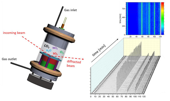
1. Introduction
Carbon Capture Utilization and Storage (CCUS) is a promising technology for the reduction of CO2 emissions from fossil-fuel-operated power plants, steel and cement mills or refineries. Carbon dioxide is captured directly at the source and is transmitted by a pipeline system either to a geological formation to be injected or to further technical processing. The most effective transmission of CO2 can be achieved in a pressurized liquid or supercritical state [1,2]. Along the process chain, pipeline steels are in contact with the stream mixture containing CO2 as the main phase and minor constituents depending on the CO2-emitting source. The type and concentration of the corrosive components depend on the combustion conditions and the following gas-processing technology [3,4]. Characteristic impurities from oxidation processes are SO2, SO3, NO2 and O2 (Oxyfuel, post-combustion) and H2S, COS and CH4 for reductive atmosphere (pre-combustion process). In general, corrosion in pipelines is insignificant if no free water in the system is present. However, in the presence of water, impurities can form acids Equations (1)–(6), which can cause harmful corrosion problems by condensation effects on steel surfaces [5,6,7,8,9,10,11,12,13,14].
Recent studies have shown that even high-alloyed steels might be susceptible to general and localized corrosion caused by these acidic condensates [6,7]. Crucial points for a sustainable and future proof CCUS procedure are reliability and cost efficiency of the pipeline transport network—in particular, regarding corrosion risks when impurities and moisture are present within the CO2 stream.
Thus, it is important to understand the corrosion rates and mechanisms of low-cost low-alloy steels in realistic transport conditions (low temperatures and low concentrations of impurities). To date, exposure tests have been performed on commercial pipeline steel grade X70 at 323 K in water-saturated supercritical CO2 and up to 2000 ppmv of O2 and/or SO2, revealing not only the chemistry of the corrosion products but also the synergistic effects between impurities on the corrosion mechanism [15,16,17]. The large number of detected phases after short reaction times reflects a multiple formation history for the generated corrosion products, mainly iron carbonate, ferrous sulfates or sulfites and hydrated ferric hydroxides.
The early stage of corrosion processes under oxidizing atmospheres at low temperatures (278–288 K), comparable with conditions in subterranean gas pipelines, is currently not well-understood. At low temperatures, the structure of corrosion products is expectedly amorphous or nanocrystalline, causing difficulties in phase analyses even with laboratory grazing incidence X-ray diffraction (GIXRD). In-situ synchrotron energy-dispersive X-ray diffraction (EDXRD) has been shown to be a powerful tool to follow the early stages of sulfidation or oxidation processes in real-time testing metal alloys [18,19,20,21,22,23,24,25]. So far, a variety of studies were carried out for corrosion processes at high temperatures (≥723 K) using high-alloyed materials in sulfurizing or oxidizing environments [18,19,20]. Ko et al. [21,22] performed in-situ synchrotron X-ray diffraction experiments to reveal the effects of microstructure and boundary layer conditions on the formation of CO2-induced corrosions’ products, mainly siderite FeCO3 and chukanovite Fe2(OH)2CO3. These experiments, however, were performed at 353K, without impurities such as NO2 and SO2, which just did not represent underground transport pipeline conditions.
Important aspects of this work were the identification of the generated phases in the early stage of corrosion and quantifying corrosion rates at a low temperature (278 K). The atmosphere used was composed of CO2 (≥99%) and the principal reactive impurities of an Oxyfuel process, namely O2, NO2, SO2 and H2O. Gas quantities were taken by calculations derived from the CLUSTER joint project (“Impacts of impurities in captured CO2 streams from different emitters of a local cluster on transport, injection and storage”) [26]. The corrosion experiments were performed at an ambient pressure and a temperature of 278 K, representing the pipeline transport conditions.
2. Materials and Methods
The selection of materials was based on results of the previous CCS research project COORAL [5]. Under comparable experimental conditions for alloyed steels (e.g., X12Cr13) and high-alloyed steels (e.g., X1NiCrMoCu32-28-7), almost no corrosion could be detected. Meanwhile, cost-efficient carbon steels demonstrate significant higher corrosion susceptibility. For this work, a high-strength carbon steel was selected, namely X70, also known as L485MB and 1.8977 in the European system. X70 is a commercially established material for natural gas pipeline constructions, whereas costly high-alloyed steels are only considered if corrosion resistance must be ensured over a longer period (e.g., in brine) [27]. The chemical composition of the investigated X70 specimens, which were sectioned from a real industrial pipeline, was determined using spark emission spectroscopy. The amounts of alloying elements are listed in Table 1. Geometry and microstructure of the X70 test specimen is presented in Figure 1. Before testing, the specimens were ground using 80, 120 and 320-grit silicon carbide abrasive paper and cleaned using ethanol and degreased by acetone to have the same starting surface conditions for all experiments.
2.1. Screening Test
Before performing the in-situ corrosion experiment at the Berlin Electron Storage Ring (Society) for Synchrotron Radiation (BESSY II, Berlin, Germany), screening tests were carried out to find out the most suitable water concentration. A detailed description of the setup and the operation method was described in prior publications [5,28]. These tests (6 h) were performed to identify the water content needed to form a thin corrosion layer covering the specimen’s surface. For this purpose, specimens were tested under conditions similar to the intended EDXRD experiment, applying an Oxyfuel atmosphere but varying moisture (50–250–1000 ppmv). To generate the desired gas atmosphere, the initial CO2 stream was split into two sub-flows. One part flew through a recipient with deionized water to achieve the desired humidity; the other part was mixed with the impurities in a swirl body. Subsequently, both flows rejoined and fed the reactor chamber. In the reactor, the specimens were exposed to a continuous stream of the CO2-impurities mixture. The experimental temperature of 278 K was adjusted by putting the reactor together with specimens into a climate chamber.
2.2. In-Situ Corrosion Experiment
The composition of the gas atmosphere in these experiments is based on the calculations of Kather et al. [29]. The concentration of corrosive impurities such as SO2, NO2 and O2 are kept as realistic as possible for future industrial applications. Due to the thermodynamic instability of the oxidizing gas mixtures in high-pressure tanks, the number of components in the applied gas atmosphere was reduced. The principal acting gases for the formation of acidic corrosion were provided in separate gas tanks containing CO2 + SO2 and CO2 + NO2 + O2. A recipient with deionized H2O was used for moistening the gas atmosphere. The experiments were run with the following final gas composition (CO2-balanced): 6700 ppmv O2, 100 ppmv NO2 and 70 ppmv SO2, thus simulating an Oxyfuel atmosphere. The moisture in screening tests was adjusted from 50 ppmv up to 1000 ppmv H2O, while, for the in-situ EDXRD experiment, a water content of 500 ppmv was employed. The applied gas atmosphere exhibited a continuous flow rate of 1 L min−1, corresponding to a flow velocity of approximately 5 cm s−1. Simulating the commonly encountered temperatures during transport, the experiments were performed at 278 K, related to the average ambient temperature in a depth of 3–5 m for subterranean pipelines in Central or Northern Europe [30]. The EDXRD experiments were performed at BESSYII at ambient pressure due to safety-relevant reasons. Furthermore, the implementation of a continuous, noncirculating flow under high pressure is hardly possible in laboratory experiments due to the huge demand of pressured fluid.
The experiment at the synchrotron beamline at BESSY II was realized in an in-house developed device (Figure 2) combining in-situ EDXRD with a corrosion experiment [18]. The experiment was performed at ambient pressure, employing a continuous flow for 15 h. The specimen was continuously cooled during the experiment to 278 K using a Peltier element. Its heat was conveyed by an aluminum block attached to a water-cooled cylinder to avoid overheating of the Peltier element (Figure 3). To control the temperature during the experiment, a thermocouple was placed inside the specimen, while another was placed next to it. Finally, the specimen was locked onto the Peltier by an aperture plate. To maintain a reference area and to avoid galvanic corrosion of the specimen in contact with the plate, a gold layer (approx. 10 nm) was deposited by a physical vapor deposition technique on the edges of the specimen before experimentation. To minimize the contamination by atmospheric oxygen, the reactor was purged with argon for 10 min before starting the EDXRD experiment. During the experiment, a continuous gas stream of the moist CO2/impurities mixture entered the reactor at the top, hit the specimen on its center and left the chamber at the bottom. After finishing the experiment, the reactor was again purged for 10 min with argon, and then, the specimen was transferred to a desiccator.
The time-resolved measurement at the energy-dispersive X-ray beamline (EDDI) at BESSY II was performed within an energy range of 10–90 keV, setting the data acquisition time to 10min/pattern. The incoming synchrotron beam passed the glassy wall of the reactor under a grazing angle of 2θ = 6. The outcoming signal was captured by a N2(l)-cooled Low-Energy Germanium (LEGe) detector (CANBERRA Ind.) with an intrinsic detector resolution of 160 eV at 10 keV and 420 eV at 100 keV. General information about the properties of the instrumentation and the major setup at the EDDI beamline are listed in [31]. To identify reaction products from the emission line positions, ICSD data [32] and the energy-dispersive Bragg Equations (7) and (8) were applied.
Ephoton = h·ν = h·c/λ
nλ = 2d·sinθ
2.3. Ex-Situ Characterization Experiments
Before and after the in-situ experiment, X-ray diffraction patterns of the blank metal surface (before the corrosion experiment) and corrosion products on the corroded specimen were collected using the Seifert PTS 3000 and applying the grazing incidence mode (GIXRD) at ω = 1, Δt = 15 s/step and Δ2θ = 0.01 using a Co tube. Further chemical, microstructural and morphological characterizations of the surface, changes caused by the corrosion process were performed by scanning electron microscope (VEGA3 TESCAN, Tescan, Czech Republic) and Zeiss-LEO Gemini 1530 (Zeiss, Oberkochen, Germany) field emission scanning electron microscope (SEM) with secondary electrons (SE) and backscattered electrons (BSE). These SEMs are equipped with energy-dispersive X-ray spectroscopy (EDS) detectors to analyze the chemical element distribution and to estimate the abundance of elements.
To assist XRD in a phase analysis of corrosion products, especially iron nitrate, a confocal Raman spectrometer (Horiba ISA Dilor LabRAM, Horiba, Japan) was used. References were taken from the RRUFF database. Focused ion beam (FIB) technique was applied to achieve a section of the interface between the steel and corrosion product, which enabled a further detailed analysis of corrosion products with scanning transmission electron microscopy (STEM; JEOL JEM2200FS, Jeol, Germany).
To calculate the general corrosion rate according to ASTM G1-03, after surface analysis, the corrosion products were removed, and the weight change was measured. Since the general corrosion rate is not reliable when pitting or localized corrosion happens, the cleaned specimen surface was characterized morphologically by interferometry (FRT MicroProf®, Fries Research & Technology Ltd. Co, Bergisch Gladbach, Germany) to map the pit depth of localized shallow pits.
3. Results
3.1. Screening Experiments
Applying 50 ppmv H2O to the gas atmosphere, after 6 h, no significant corrosion effects on the specimen surface were observed. By raising the water content up to 250 ppmv, small, isolated corrosion spots were formed, mostly associated with grinding marks. Increasing the water content up to 1000 ppmv resulted in an almost closed corrosion layer developed by connecting local corrosion spots (Figure 4). Cross sections of this corrosion layer revealed an average thickness of 80 to 100 nm. The rounded shape of the corrosion spots was interpreted as condensed acid droplets derived from the moist atmosphere by experimenting below the acid dew points of H2SO4 and HNO3, respectively [6,33]. The spots accumulated preferentially along grinding marks, as can be seen clearly in Figure 5. This could be explained by the higher probability for the presence of steps or kinks, which are thermodynamically favorable for the adsorption of droplets due to their lower surface energy [34]. Based on this observation, in the in-situ corrosion experiment, a water content of 500 ppmv was applied to obtain a closed, thin corrosion layer after 15 h under same experimental conditions.
3.2. In-Situ corrosion Experiment
In-situ corrosion experiments were performed at the “BESSY II” synchrotron beamline applying Oxyfuel atmosphere (278 K, 1bar) for 15 h. Due to chemical reactions of X70 with the moist oxidizing gas atmosphere, a thin corrosion layer with golden-brownish color was generated on the surface (Figure 6). From this figure, it can be seen that the beam was entering from the left side, touching the specimen’s surface in the center and then leaving off at the right side, generating a distinctly altered zone due to its high energy. Obviously, the measuring beam itself might alter the structure of the growing corrosion products, where the amount of alternation is unknown at this point. The morphological differences between these zones are analyzed and discussed in the following section.
Figure 7 shows time-resolved diffraction patterns recorded during an in-situ corrosion experiment. The intensities of the reflected emission lines are color-coded, ranging from red (high intensity) to blue (low intensity). Considering the complete spectrum (Figure 7a), all recognizable emission lines can be assigned to elements scattered by radiation on the measuring equipment (escape peaks stemming from the Ge detector around 10 keV) or provoked by the bulk material of the specimen (α-ferrite: 58.3; 82.3 and 100.8 keV) [18,31]. The sharpness and high intensity of these lines point at a high crystallinity, and their large number is attributed to numerous electron transfers between different orbitals [34]. Due to these strong signals, the X-ray diffraction signals of corrosion products probably are covered or hidden by the elevated background. By magnification of the energy range 15–45 keV and customizing the intensity spectrum, further emission lines with low signal strengths were identified (Figure 7b–d). Due to the number, signal weakness and width of these patterns, it can be concluded that only a small fraction of the corrosion products is crystalline and the majority is X-ray-amorphous. A total of five signals can be identified, which are located at 20.10 keV, 26.35 keV, 31.81 keV, 36.35 keV and 40.18 keV. Three different starting points (around 150 min, 240 min and 360 min) indicating the presence of various phases or, rather, the formation of preferred crystallographic orientations.
Based on the energy-dispersive Bragg-equation, Equations (7) and (8) and the use of ICSD data [32] the reflected EDXRD signals can be allocated to specific phases (Table 2). Table 2 lists the corrosion phases detected by in-situ EDXRD, including the energy of the emission line and their onset time. Based on the position of the emission lines, the generated phases could be allocated to different water-bearing iron sulfates, namely Lausenite, Rozenite and Meta-hohmannite. The first reflection signal started around 150 min (located at 36.35 keV) and can be assigned to the (30
) reflex of Lausenite (Fe2(SO4)3·5H2O; COD 900-3639). The signal strength is very weak and not increased with time, as it is not a significant phase. After 240 min, another low-intensity peak slowly starts to increase with time. The signal position is located at 26.35 keV, which can be related to the (111) reflex of Rozenite (FeSO4·4 H2O; COD 900-7474). Around 360min, more pronounced emission lines begin to grow at 20.10 keV, 31.81 keV and 40.18 keV. Due to their energy positions, they can be referred to as Metahohmannite (Fe2(SO4)2O·4H2O; COD 900-3333). The intensity of these emission lines decreases slightly with time, suggesting consumption by other phases, most likely amorphous due to a lack of further emission lines. Due to the few and low-intensity reflection signals, an unambiguous assignment of the reflexes to phases is only possible to a limited extent. Further characteristic peaks of the corrosion products are presumably covered by the high background or peaks induced by the equipment.
After the in-situ corrosion experiment, the slightly wet specimen surface was tested by a pH indicator (Macherey-Nagel GmbH & Co. KG), suggesting a value around pH 1.5. This result agrees with comparable experiments by Ruhl et al., in which pH values less than 2 were observed [10]. As mentioned above, a driving force for the formation of corrosion products is the presence of acidic droplets.
Analyses of acid residues from comparable experiments showed that the major fraction is H2SO4 (>90%) and only a small part is HNO3 [6,10]. The reason for this might be that NO2 mainly acts as an oxidizing agent, converting SO2 into SO3 so that only a small part is available for the formation of HNO3. Since the experiments were carried out below the dew point of H2SO4, presumably small acid droplets were formed in the atmosphere [33,34]. Further evidence of the acid formation and the catalytic role of NO2 have been further proved, even under higher pressure by recent works from Morland et al. [35,36,37]. These acids condensed at the specimen’s surface, being the coldest point in the system due to the Peltier element underneath. Iron atoms close to the surface were reacted, dissolved and mobilized by acid solutions. Chemical reactions and the crystallization of iron sulphate phases can be described and simplified in Equations (9) and (10).
The phases formed in the in-situ corrosion experiment are water-bearing iron sulfates, slightly differing in terms of the incorporated amount of water. This may be caused by different diffusion coefficients or a limited transport due to the low moisture content in the gas atmosphere.
The initially generated phases, namely Lausenite and Rozenite, are characterized by a monocline crystal system in which iron octahedra are linked to sulfate tetrahedra. Both phases exhibit large lattice parameters: Lausenite (P21/m; a = 10.68Å, b = 11.05Å and c = 5.57Å) and Rozenite (P21/b; a = 5.98Å, b = 13.65Å and c = 7.98Å) [38,39]. The latter formed Metahohmannite crystallizes in the tricline space group. The structure is similar to the previously generated phases, by linking four Fe3+ octahedra and four sulfate tetrahedra. The lattice parameters are large as well, showing a = 7.35Å, b = 9.77Å and c = 7.15Å [40]. Due to the large unit cells and the presence of structural channels [39,40], these phases can incorporate large molecules, such as H2O (rcovalent = 1.67Å) [41], SO2 (rcovalent = 2.15Å) [42], O2 (rcovalent = 1.40Å) [41], O2− (rionic = 1.26Å) [43], OH−(rionic = 1.37 Å) [44] or SO42− (rionic = 2.58Å) [45].
For the microstructural-chemical characterization, SEM/EDS and TEM were carried out. It became obvious that the corroded specimen was covered by a thin layer of products with an average thickness of 0.2 µm and locally grown globular structures up to 10 µm in diameter (Figure 8). Characteristic features of the globular structures are numerous cavities (≤0.5 µm) or cracks (≤1.0 µm), mostly situated at the interface with the layer (Figure 8). Reasons for cracking could be dehydration or processes of degassing induced by the vacuum in electron microscopy. Considering the interface steel/corrosion layer, no pitting corrosion was observed, which was also reported for comparable experiments [6,10,28]. Figure 9 presents the EDS elemental analysis of the area that interacted with the beam, again proving the existence of S and O as main elements of the water-bearing iron sulphate corrosion products.
To further analyze corrosion products with scanning transmission electron microscopy (STEM), the focused ion beam (FIB) technique was applied to achieve a section image of the interface between the steel and corrosion product. The corrosion layer between the ferritic-pearlitic steel below and a protective platinum deposition above is shown in Figure 10. Backscattered electron (BSE) images showed no contrast between the thin layer and the globular structures, indicating a similar chemical composition. Higher magnification of the globular structures by STEM mode demonstrates small spotted areas with brighter or darker color contrasts than the surrounding material (Figure 10), indicating differences in the chemical compositions.
A variability of the chemical composition for Fe (25–32 at %), S (18–24 at %) and O (32–49 at %) can be observed by EDX for the corrosion products (Figure 9). Line scan indicated that oxygen and sulfur tend to be chemically coupled, caused by the formation of sulfate (SO42−). The large range for oxygen can be explained by the different amounts of H2O in the water-bearing phases. Changes in the element ratio Fe:S:O could be observed on a small scale, which points to a very fine-grained intergrown of different phases (Figure 11). Concerning the spotted areas in the BSE images, darker spots are enriched in sulfur and oxygen, while brighter spots are more ferrous. Further alloying elements of X70, such as Cr, Mn, C and Si, were below the measurement sensitivity (≤1 wt %). To verify the crystallinity at the interface steel/corrosion layer, investigations in STEM mode were performed (Figure 12). For the bare metal surface (X70), a sharp nanobeam diffraction pattern (spot size 0.5 nm) could be observed; meanwhile, the pattern of the corrosion layer showed annular structures made of small, blurred reflexes, which are known for amorphous or nanocrystalline materials.
Since characterization by XRD, SEM and TEM demonstrated that the corrosion products were chemically variable and mainly R-ray amorphous, investigations by Raman spectroscopy were carried out for further phase identification. The Raman spectra were recorded in the range of 200–1750 cm−1 and 2800–3700 cm−1 using a Nd:YAG laser at 532 nm. The confocal hole was 400 µm, and the spectral slit width was 100 µm, resulting in a spectral resolution of 4.5 cm−1. To avoid phase changes in the corrosion layer during measurements, the specimen was irradiated with a low energy density of 3mWcm−2. The investigations show three different spectra: one was assigned to the corrosion layer and two allocated to globular structures on top (Figure 13). The Raman spectrum of the corrosion layer cannot be assigned clearly to one phase. Some of the identifiable bands very strongly overlapped with others, indicating a mixed spectrum of different phases. A general distinction can be made between iron nitrates and iron sulfates, both very likely water-bearing phases, which can be assumed from the OH-stretching modes at high wave numbers [46]. Precise phase identification was hardly possible, since both sulfates and nitrates are chemical-structurally similar [47,48,49,50], with results for Raman bands in almost the same number and energy position. The Raman bands differ slightly in terms of the incorporated contents of the crystallization water, which leads to band shifts. The smaller the wave numbers, the lower is the water content of the phase [49,50]. The broad Raman bands and the high background indicate very fine-grained/nanocrystalline phases that are intergrown.
Concerning the globular structures on top of the corrosion layer, it was possible to distinguish dark (minority) and white-yellowish (majority) formations using optical microscopy. These are also reflected in the Raman spectra (Figure 13) and were clearly assigned to Hematite (α-Fe2O3) and Rozenite (FeSO4·4H2O) [49,51]. The water-bearing character of Rozenite is confirmed by the broad Raman bands in the range of 3000 to 3600 cm−1 assigned to OH-stretching vibrations [46].
To reveal the formation tendency of corrosion products in the same condition (100 ppmv NO2 + 70 ppmv SO2 + 6700 ppmv O2, 1 bar and 278 K), a long-term test was carried out up to 168h with an increased water content (8000 ppmv). In comparison to the corroded specimen from the in-situ short-term corrosion experiment, the ex-situ grazing incidence X-ray (GIXRD) result (Figure 14) of the long-term corroded specimen shows additional phases, namely Mikasaite (Fe2(SO4)3; COD 900-8259), Hohmannite (Fe2[O(SO4)2]·8H2O; COD 901-1796) and Ferricopiapite (Fe5(SO4)6(OH)2·20H2O; COD 900-0307). Furthermore, with increasing time, the crystalline fraction and the grain size of the corrosion products ascend significantly, presented by the higher number and smaller full-width half-maximum (FWHM) of the detected peaks. Experiments by Ruhl et al. [10] under comparable gas atmosphere and p-T conditions also showed various water-bearing iron sulfates as corrosion products. However, the chemical compositions of those phases are different from those found in this study. This is probably due to the higher contents of SO2 and NO2 in their experiments, which resulted in acids with different concentrations followed by alternative phase formation.
To determine the corrosion rate during the in-situ corrosion experiment, the mass loss of the specimen was determined. For this purpose, the weight difference of the specimen before and after the experiment was quantified and related to the reacted specimen surface. To remove the corrosion products from the surface, the specimen was immersed in etching solution for 10 seconds and then mechanically detached. The corrosion rate v was calculated using Equation (11),
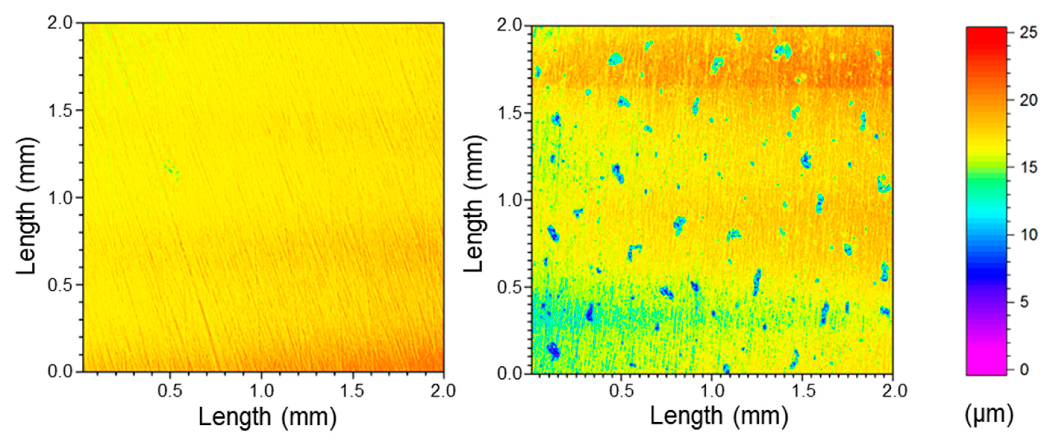
where v is the corrosion rate in mm/a, K is a conversion constant (87,600), Δm is the weight loss in g, ρ is the density of the specimen in g/cm3, A is the reacted area in cm2 and t is the experimental time in h. The calculated corrosion rate was 0.09 mm/a, which roughly corresponds to the results by SEM/TEM estimating the average thickness of the corrosion layer in relation to the experiment duration (≤0.12 mm/a). In a last step, the cleaned specimen surface was characterized morphologically by interferometry. Compared to the unreacted area on the specimen surface, the corroded area displays shallow pits (Figure 15). In general, these pits are related to grinding marks and are developed elongated. The lateral dimensions range within 60–120 µm × 30–60 µm, and density of the pits was around 7.5 × 10⁶ m−2. The depth of the pits was up to 15 µm.
v = (K·Δ m)/(ρ·A·t)
Comparable experiments on low carbon steel, such as X70, also showed shallow pitting as the corrosion type, demonstrating similar dimensions and densities for pitting [6,33,52]. The calculated corrosion rate of this work was between results of wet-chemical (0.5×) [6] and gas-chemical (40×) [53,54] investigations. This indicates a permanently wet surface during the experiment, leading to a continuously progressing and homogeneous corrosion.
4. Conclusions
As an attempt to investigate the early stage of the corrosion process that happens on pipeline steel X70 for CO2 transport, an in-situ synchrotron EDXRD experiment was carried out in a continuous flow of simulated Oxyfuel atmosphere (6700 ppmv O2, 100 ppmv NO2, 70 ppmv SO2, 500 ppmv H2O and balanced CO2) at 278K and ambient pressure for 15h. The corrosion products were characterized in real time using in-situ EDXRD and afterward by GIXRD, FIB/SEM/TEM, EDX and Raman spectroscopy. It became apparent that a large fraction of the corrosion products was amorphous and only a small part was crystalline/nanocrystalline. The crystalline part was detected by EDXRD and allocated to the formation of water-bearing iron sulfates, namely Lausenite, Rozenite and Metahohmannite. These results were further proven by EDS points and line scan, which showed the chemical coupling of O and S in the corrosion products, corresponding with the formation of sulfates (SO42−).
Investigation by Raman spectroscopy confirmed the presence of water-bearing sulfates but verified also the formation of small amounts of nitrates in the corrosion layer. The source of corrosion was the generation of acid droplets (pH 1.5) in the gas atmosphere due to gaseous cross-reactions and the temperature below the dewpoints of H2SO4 and HNO3. Droplets condensed on the specimen surface, provoking chemical reactions with the material. The corrosion started locally at grinding marks with the formation of small corrosion spots. With an increasing experiment duration or moisture content, the corrosion process proceeded until a closed corrosion layer had been formed. In addition, globular structures were formed on the surface of the corrosion layer.
Supplementary long-term tests pointed out a significant ascent of the crystalline fraction in the corrosion layer with increasing experimental time. In addition, the formation of further water-bearing iron sulfates could be observed, namely Mikasaite, Metahohmannite and Ferricopiapite. For the globular structures on top of the layer, a minor part of Hematite (α-Fe2O3) and the major part of Rozenite (FeSO4·4H2O) were proven. The formation of those could be explained by small changes in the gas atmosphere at the end of the in-situ experiment or by phase transformation afterwards. Since the chemical composition within the corrosion layer varies in the nanometer range, a very fine network of different phases is assumed. This nanocrystalline/amorphous character of the corrosion products in the early stage of formation was confirmed by STEM (scanning transmission electron microscopy).
Author Contributions
Conceptualization, A.K. and D.B.; investigation, A.K. and M.M.; methodology, A.K.; project administration, D.B.; validation, A.K.; writing—original draft, A.K.; writing—review and editing, L.Q.H., D.B. and R.B. All authors have read and agreed to the published version of the manuscript.
Funding
This research was funded by German Federal Ministry for Economic Affairs and Energy, grant number FKZ 03ET7031C, in Project CLUSTER.
Acknowledgments
The authors would like to acknowledge Helmholtz-Zentrum Berlin for the allocation of synchrotron beamtime at BESSY II, Christiane Stephan-Scherb (BAM) for supervising, planning, and applying to get the beam time in BESSY II, Christoph Peetz for carrying out the screening experiments, Axel Kranzmann for discussion and hints, Manuela Klaus (HZB) for the technical support and helpful discussions at BESSY II, Romeo Saliwan Neumann (BAM) for SEM analysis, Ines Häussler for realizing TEM measurements and Nicole Wollschläger (BAM) for the preparation of TEM lamella.
Conflicts of Interest
The authors declare no conflicts of interest.
References
- Gale, J.; Davison, J. Transmission of CO2—Safety and economic considerations. Energy 2004, 29, 1319–1328. [Google Scholar] [CrossRef]
- Vandeginste, V.; Piessens, K. Pipeline design for a least-cost router application for CO2 transport in the CO2 sequestration cycle. Int. J. Greenh. Gas Control 2008, 2, 571–581. [Google Scholar] [CrossRef]
- Fleig, D.; Normann, F.; Andersson, K.; Johnsson, F.; Leckner, B. The fate of sulphur during oxyfuel combustion of lignite. Energy Procedia 2009, 9, 383–390. [Google Scholar] [CrossRef] [Green Version]
- Lee, J.Y.; Keener, T.C.; Yang, Y.J. Potential Flue Gas Impurities in Carbon Dioxide Streams Separated from Coal-Fired Power Plants. J. Air Waste Manag. Assoc. 2009, 59, 725–732. [Google Scholar] [CrossRef] [PubMed]
- Rütters, H.; Stadler, S.; Bäßler, R.; Bettge, D.; Jeschke, S.; Kather, A.; Lempp, C.; Lubenau, U.; Ostertag-Henning, C.; Schmitz, S.; et al. Towards an optimization of the CO2 stream composition—A whole-chain approach. Int. J. Greenh. Gas Control 2016, 54, 682–701. [Google Scholar] [CrossRef]
- Yevtushenko, O.; Bettge, D.; Bäßler, R.; Bohraus, S. Corrosion of CO2 transport and injection pipeline steels due to the condensation effects caused by SO2 and NO2 impurities. Mater. Corros. 2015, 66, 334–341. [Google Scholar] [CrossRef]
- Quynh Hoa, L.; Baessler, R.; Bettge, D. On the Corrosion Mechanism of CO2 Transport Pipeline Steel Caused by Condensate: Synergistic Effects of NO2 and SO2. Materials 2019, 12, 364. [Google Scholar] [CrossRef] [Green Version]
- Choi, Y.-S.; Nesic, S.; Young, D. Effect of Impurities on the Corrosion Behavior of CO2 Transmission Pipeline Steel in Supercritical CO2-Water Environments. Environ. Sci. Technol. 2010, 44, 9233–9238. [Google Scholar] [CrossRef]
- Xiang, Y.; Wang, Z.; Xu, C.; Zhou, C.; Li, Z.; Ni, W. Impact of SO2 concentration on the corrosion rate of X70 steel and iron in water-saturated supercritical CO2 mixed with SO2. J. Supercrit. Fluids 2011, 58, 286–294. [Google Scholar] [CrossRef]
- Ruhl, A.S.; Kranzmann, A. Corrosion behavior of various steels in a continuous flow of carbon dioxide containing impurities. Int. J. Greenh. Gas Control 2012, 9, 85–90. [Google Scholar] [CrossRef]
- Morland, B.H.; Dugstad, A.; Svenningsen, G. Corrosion of Carbon Steel in Dense Phase CO2 with Water above and Below the Solubility Limit. Energy Procedia 2017, 114, 6752–6765. [Google Scholar] [CrossRef]
- Halseid, M.; Dugstad, A.; Morland, B.H. Corrosion and Bulk Phase Reactions in CO2 Transport Pipelines with Impurities: Review of Recent Published Studies. Energy Procedia 2014, 63, 2557–2569. [Google Scholar] [CrossRef] [Green Version]
- Lan, T.T.N.; Thoa, N.T.P.; Nishimura, R.; Tsujino, Y.; Yokoi, M.; Maeda, Y. Atmospheric corrosion of carbon steel under field exposure in the southern part of Vietnam. Corros. Sci. 2006, 48, 179–192. [Google Scholar] [CrossRef]
- Syed, S. Atmospheric corrosion of hot and cold rolled carbon steel under field exposure in Saudi Arabia. Corros. Sci. 2008, 50, 1779–1784. [Google Scholar] [CrossRef]
- Wei, L.; Pang, X.; Gao, K. Effect of flow rate on localized corrosion of X70 steel in supercritical CO2 environments. Corros. Sci. 2018, 136, 339–351. [Google Scholar] [CrossRef]
- Sun, J.; Sun, C.; Wang, Y. Effects of O2 and SO2 on Water Chemistry Characteristics and Corrosion Behavior of X70 Pipeline Steel in Supercritical CO2 Transport System. Ind. Eng. Chem. Res. 2018, 57, 2365–2375. [Google Scholar] [CrossRef]
- Qin, F.; Jiang, C.; Cui, X.; Wang, Q.; Wang, J.; Huang, R.; Yu, D.; Qu, Q.; Zhang, Y.; Peng, P.D. Effect of soil moisture content on corrosion behavior of X70 steel. Int. J. Electrochem. Sci. 2018, 13, 1603–1613. [Google Scholar] [CrossRef]
- Falk, F.; Menneken, M.; Stephan-Scherb, C. Real-Time Observation of High-Temperature Gas Corrosion in Dry and Wet SO2-Containing Atmosphere. JOM 2019, 71, 1560–1565. [Google Scholar] [CrossRef] [Green Version]
- Stephan-Scherb, C.; Nützmann, K.; Kranzmann, A.; Klaus, M.; Genzel, C. Real time observation of high temperature oxidation and sulfidation of Fe-Cr model alloys. Mater. Corros. 2018, 69, 678–689. [Google Scholar] [CrossRef]
- Okoro, S.C.; Niessen, F.; Villa, M.; Apel, D.; Montgomery, M.; Frandsen, F.J.; Pantleon, K. Complementary Methods for the Characterization of Corrosion Products on a Plant-Exposed Superheater Tube. Metallogr. Microstruct. Anal. 2017, 6, 22–35. [Google Scholar] [CrossRef] [Green Version]
- Ko, M.; Ingham, B.; Laycock, N.; Williams, D.E. In situ Synchrotron X-ray diffraction study of the effect of microstructure and boundary layer conditions on CO2 corrosion of pipeline steels. Corros. Sci. 2015, 90, 192–201. [Google Scholar] [CrossRef] [Green Version]
- Ko, M.; Ingham, B.; Laycock, N.; Williams, D.E. In situ Synchrotron X-ray diffraction study of the effect of chromium additions to the steel and solution on CO2 corrosion of pipeline steels. Corros. Sci. 2014, 80, 237–246. [Google Scholar] [CrossRef]
- Hassan Sk, M.; Abdullah, A.M. Corrosion of General Oil-field Grade Steel in CO2 Environment—An Update in the Light of Current Understanding. Int. J. Electrochem. Sci. 2017, 12, 4277–4290. [Google Scholar] [CrossRef] [Green Version]
- Ja’baz, I.; Jiao, F.; Wu, X.; Yu, D.; Ninomiya, Y.; Zhang, L. Influence of gaseous SO2 and sulphate-bearing ash deposits on the high-temperature corrosion of heat exchanger tube during oxyfuel combustion. Fuel Process. Technol. 2017, 167, 193–204. [Google Scholar] [CrossRef]
- Ghahari, M.; Krouse, D.; Laycock, N.; Rayment, T.; Padovani, C.; Stampanoni, M.; Marone, F.; Mokso, R.; Davenport, A.J. Synchrotron X-ray radiography studies of pitting corrosion of stainless steel: Extraction of pit propagation parameters. Corros. Sci. 2015, 100, 23–35. [Google Scholar] [CrossRef] [Green Version]
- CLUSTER—Impacts of Impurities in CO2 Streams Captured from Different Emitters in a Regional Cluster on Transport, Injection and Storage. Available online: www.bgr.bund.de/CLUSTER-EN (accessed on 1 May 2019).
- Schutz, R.W.; Watkins, H.B. Recent developments in titanium alloy application in the energy industry. Mater. Sci. Eng. A 1998, 243, 305–315. [Google Scholar] [CrossRef]
- Ruhl, A.S.; Kranzmann, A. Investigation of corrosive effects of sulphur dioxide, oxygen and water vapour on pipeline steels. Int. J. Greenh. Gas Control 2013, 13, 9–16. [Google Scholar] [CrossRef]
- Engel, F.; Kather, A. Conditioning of a Pipeline CO2 Stream for Ship Transport from Various CO2 Sources. Energy Procedia 2017, 114, 6741–6751. [Google Scholar] [CrossRef]
- Bodentemperatur. Available online: https://www.pik-potsdam.de/services/klima-wetter-potsdam/klimazeitreihen/bodentemperatur (accessed on 1 May 2019).
- Genzel, C.; Denks, I.A.; Gibmeier, J.; Klaus, M.; Wagener, G. The materials science Synchrotron beamline EDDI for energy-dispersive diffraction analysis. Nucl. Instrum. Meth. Phys. Res. A 2007, 578, 23–33. [Google Scholar] [CrossRef]
- ICSD-Fiz-Karlsruhe Inorganic Crystal Structure Database. Available online: https://www.fiz-karlsruhe.de/en/produkte-und-dienstleistungen/inorganic-crystal-structure-database-icsd (accessed on 1 May 2019).
- Huijbregts, W.M.M.; Leferink, R.G.I. Latest advances in the understanding of acid dewpoint corrosion: Corrosion and stress corrosion cracking in combustion gas condensates. Anti-Corros. Methods Mater. 2004, 51, 173–188. [Google Scholar] [CrossRef] [Green Version]
- Atkins, P.; Paula, J.; Keeler, J. Physical Chemistry, 11th ed.; Oxford University Press: Oxford, UK, 2018. [Google Scholar]
- Morland, B.H.; Norby, T.; Tjelta, M.; Svenningsen, G. Effect of SO2, O2, NO2, and H2O concentrations on chemical reactions and corrosion of carbon steel in dense phase CO2. Corrosion 2019, 75, 1327–1338. [Google Scholar] [CrossRef] [Green Version]
- Morland, B.H.; Tjelta, M.; Norby, T.; Svenningsen, G. Acid reactions in hub systems consisting of separate non-reactive CO2 transport lines. Int. J. Greenh. Gas Control 2019, 87, 246–255. [Google Scholar] [CrossRef]
- Morland, B.H.; Tadesse, A.; Svenningsen, G.; Springer, R.D.; Anderko, A. Nitric and Sulfuric Acid Solubility in Dense Phase CO2. Ind. Eng. Chem. Res. 2019, 58, 22924–22933. [Google Scholar] [CrossRef]
- Majzlan, J.; Botez, C.; Stephens, P.W. The crystal structures of synthetics Fe2(SO4)3(H2O)5 and the type specimen of lausenite. Am. Mineral. 2005, 90, 411–416. [Google Scholar] [CrossRef]
- Ackermann, A.; Lazic, B.; Armbruster, T.; Doyle, S.; Grevel, K.-S.; Majzlan, J. Thermodynamic and crystallographic properties of kornelite [Fe2(SO4)3-7.75H2O] and paracoquimbite [Fe2(SO4)3·9H2O]. Am. Mineral. 2009, 94, 1620–1628. [Google Scholar] [CrossRef]
- Scordari, F.; Ventruti, G.; Gualtieri, A.F. The structure of metahohmannite, Fe23 + [O(SO4)2]·4H2O, by in situ Synchrotron powder diffraction. Am. Mineral. 2004, 89, 365–370. [Google Scholar] [CrossRef]
- Kammeyer, C.W.; Whitman, D.R. Quantum Mechanical Calculation of Molecular Radii. I. Hydrides of Elements of Periodic Groups IV through VII. J. Chem. Phys. 1972, 56, 4419–4421. [Google Scholar] [CrossRef] [Green Version]
- Matito-Martos, I.; Martin-Calvo, A.; Gutierrez-Sevillano, J.J.; Haranczyk, M.; Doblare, M.; Parra, J.B.; Ania, C.O.; Calero, S. Zeolite screening for the separation of gas mixtures containing SO2, CO2 and CO. Phys. Chem. Chem. Phys. 2014, 16, 19884–19893. [Google Scholar] [CrossRef] [Green Version]
- Shannon, R.D. Revised Effective Ionic Radii and Systematic Studies of Interatomie Distances in Halides and Chaleogenides. Acta Cryst. 1976, A32, 751–767. [Google Scholar] [CrossRef]
- Ribbe, P.H.; Gibbs, G.H. Crystal Structures of the Humite Minerals: III. Mg/Fe Ordering in Humite and its Relation to Other Ferromagnesian Silicates. Am. Mineral. 1971, 56, 1155–1173. [Google Scholar]
- Jenkins, H.D.B.; Thakur, K.P. Reappraisal of thermochemical radii for complex ions. J. Chem. Educ. 1979, 56, 576–577. [Google Scholar] [CrossRef]
- Sun, Q.; Zheng, H. Raman OH stretching vibration of ice Ih. Prog. Nat. Sci. 2009, 19, 1651–1654. [Google Scholar] [CrossRef]
- Sharma, S.K. Raman study of ferric nitrate crystalline hydrate and variably hydrated liquids. J. Chem. Phys. 1974, 61, 1748–1754. [Google Scholar] [CrossRef]
- Hua, Y.; Barker, R.; Neville, A. Corrosion behaviour of X65 steels in water-containing supercritical CO2 environments with NO2/O2. In Proceedings of the CORROSION 2018, NACE International, Phoenix, AZ, USA, 15–19 April 2018; p. 11085. [Google Scholar]
- Chio, C.H.; Sharma, S.K.; Muenow, D.W. The hydrates and deuterates of ferrous sulfate (FeSO4): A Raman spectroscopic study. J. Raman Spectrosc. 2007, 38, 87–99. [Google Scholar] [CrossRef]
- Chio, C.H.; Sharma, S.K.; Muenow, D.W. Micro-Raman studies of hydrous ferrous sulfates and jarosites. Spectrochim. Acta A 2005, 61, 2428–2433. [Google Scholar] [CrossRef]
- Chourpa, I.; Douziech-Eyrolles, L.; Ngaboni-Okassa, L.; Fouquenet, J.F.; Cohen-Jonathan, S.; Souce, M.; Marchais, H.; Dubois, P. Molecular composition of iron oxide nanoparticles, precursors for magnetic drug targeting, as characterized by confocal Raman microspectroscopy. Analyst 2005, 130, 1395–1403. [Google Scholar] [CrossRef]
- Hua, Y.; Barker, R.; Neville, A. Understanding the Influence of SO2 and O2 on the Corrosion of Carbon Steel in Water-Saturated Supercritical CO2. Corrosion 2014, 71, 667–683. [Google Scholar] [CrossRef]
- Ruhl, A.S.; Goebel, A.; Kranzmann, A. Corrosion Behavior of Various Steels for Compression, Transport and Injection for Carbon Capture and Storage. Energy Procedia 2012, 23, 216–225. [Google Scholar] [CrossRef] [Green Version]
- Le, Q.H.; Baessler, R.; Knauer, S.; Jaeger, P.; Kratzig, A.; Bettge, D.; Kranzmann, A. Droplet Corrosion of CO2 Transport Pipeline Steels in Simulated Oxyfuel Flue Gas. Corrosion 2018, 74, 1406–1420. [Google Scholar] [CrossRef]
Figure 1.
Left: Geometry of the specimens (X70) used in the corrosion experiments. Right: Optical microscope image after polishing and etching, showing the ferritic-pearlitic microstructure of X70.
Figure 1.
Left: Geometry of the specimens (X70) used in the corrosion experiments. Right: Optical microscope image after polishing and etching, showing the ferritic-pearlitic microstructure of X70.

Figure 2.
Setup of the experimental chamber: schematic design (left) and the real test system (right). The inlets for the gas mixture and the thermocouples (TE) are located at the top, while the gas outlet and electric cables are at the lower part. The walls are made of quartz glass, so the incoming beam can enter the chamber under a fixed small angle. The radiation hits the centered specimen, which is mounted on a specific cooling system (Figure 3).

Figure 3.
Inside of the test chamber with a test specimen mounted on a Peltier element (PE), fixing aperture unmounted. To remove the induced heat, the backside of the Peltier is coupled on an aluminum cylinder (Al) conducting the thermal energy to the water-cooled steel bottom of the chamber.
Figure 3.
Inside of the test chamber with a test specimen mounted on a Peltier element (PE), fixing aperture unmounted. To remove the induced heat, the backside of the Peltier is coupled on an aluminum cylinder (Al) conducting the thermal energy to the water-cooled steel bottom of the chamber.

Figure 4.
Specimens of X70 after short-term (6 h) corrosion experiments applying Oxyfuel atmosphere (100 ppmv NO2 + 70 ppmv SO2 + 6700 ppmv O2, 1 bar and 278 K) with different water contents. The upper pictures show the macroscopic surfaces; the lower pictures show the microscopic topology (taken by a light microscope). With increasing moisture in the employed gas atmosphere, the formation of localized corrosion rises clearly.
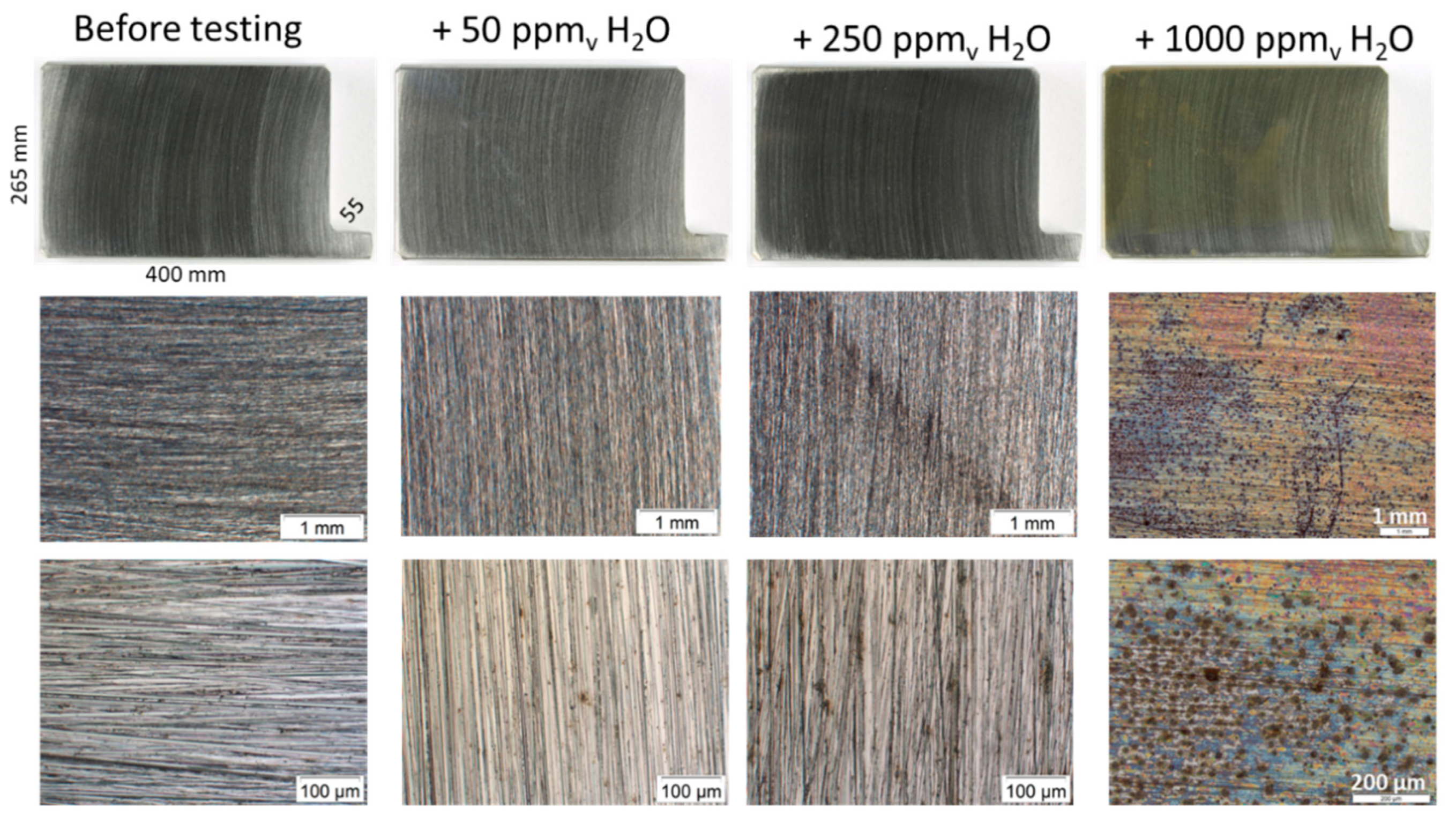
Figure 5.
(a,c) Secondary electron images (SEM) and (b,d) corresponding backscattered electron (BSE) images of the corroded specimens in the screening test (Figure 4) under 1000 ppmv H2O, 100 ppmv NO2 + 70ppmv SO2 + 6700ppmv O2, 1 bar and 278K. (c,d) show the details of (a,b), respectively.
Figure 5.
(a,c) Secondary electron images (SEM) and (b,d) corresponding backscattered electron (BSE) images of the corroded specimens in the screening test (Figure 4) under 1000 ppmv H2O, 100 ppmv NO2 + 70ppmv SO2 + 6700ppmv O2, 1 bar and 278K. (c,d) show the details of (a,b), respectively.

Figure 6.
Photograph of a specimen after an in-situ energy-dispersive X-ray diffraction (EDXRD) experiment in an Oxyfuel atmosphere at 278 K and 1 bar for 15 h. The circular spot on the surface of the specimen reveals the reaction zone generated during the corrosion experiment. On the left and right margins of the specimen, the thin Au layer are still visible. The beam was entering from the left side, touching in the center and then leaving off the right side, generating a distinctly altered zone.
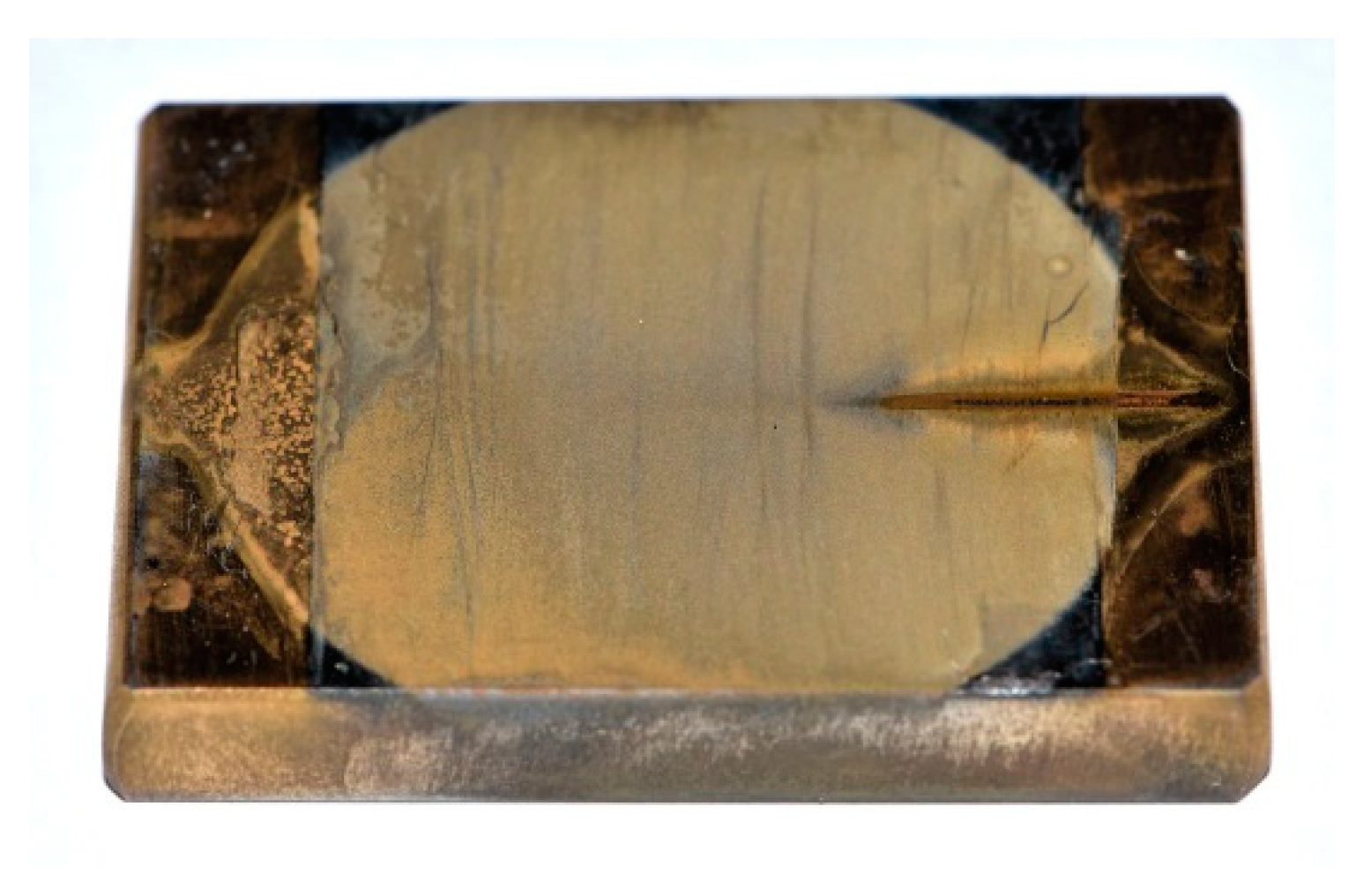
Figure 7.
Time-resolved EDXRD spectra of the pipeline steel X70 treated for 900 min (15 h) in an Oxyfuel atmosphere containing moisture of 500 ppmv. The relative intensity of the emission lines can be deviated by the lateral bar ranging from red (high) to blue (low). Allocated elements or phases are indexed above. (a) Complete spectrum of X70 (0–120 keV). In the range of 15–45 keV, the level of intensity according to the existing emission lines is displayed in the graphics. (b–d) Magnified spectrum of X70 in the range of 15–25 keV. Around 20 keV, an emission line is visible starting at approx. 390 min and getting weaker by the time. (c) Magnified spectrum of X70 in the range of 25–35 keV. Very weak emission lines can be observed at 26.3 keV and 31.8 keV. (d) Magnified spectrum of X70 in the range of 35–45 keV. A significant emission line around 40.2 keV, as well as two very weak lines at 36.3 keV and 39.1 keV, are in evidence.

Figure 8.
(a) Photograph of the specimen after EDXRD, (c,b) BSE and (e,d) secondary electron (SE) images of the corrosion layer on top of the in-situ EDXRD specimen (X70). Two different zones are presented: in the middle of specimen (c,e) and the altered zones (b,d).
Figure 8.
(a) Photograph of the specimen after EDXRD, (c,b) BSE and (e,d) secondary electron (SE) images of the corrosion layer on top of the in-situ EDXRD specimen (X70). Two different zones are presented: in the middle of specimen (c,e) and the altered zones (b,d).
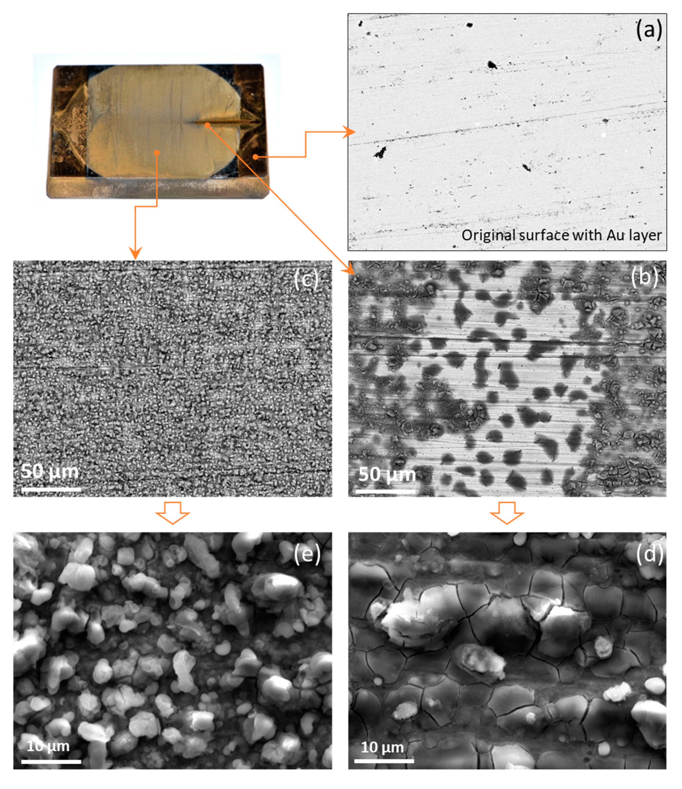
Figure 9.
BSE image and energy-dispersive X-ray spectroscopy (EDS) analysis of the corrosion products in the region presented in Figure 8b. Spectrum 1 shows the result of the corrosion product, presented as a darker region in the BSE image (a). (c) Spectrum 2 shows the data of a very hell region in the BSE image, mostly metal substrates with a very thin corrosion product indicated by a high intensity of an Fe peak and low intensity of S and O peaks as compared to that of spectrum 1.
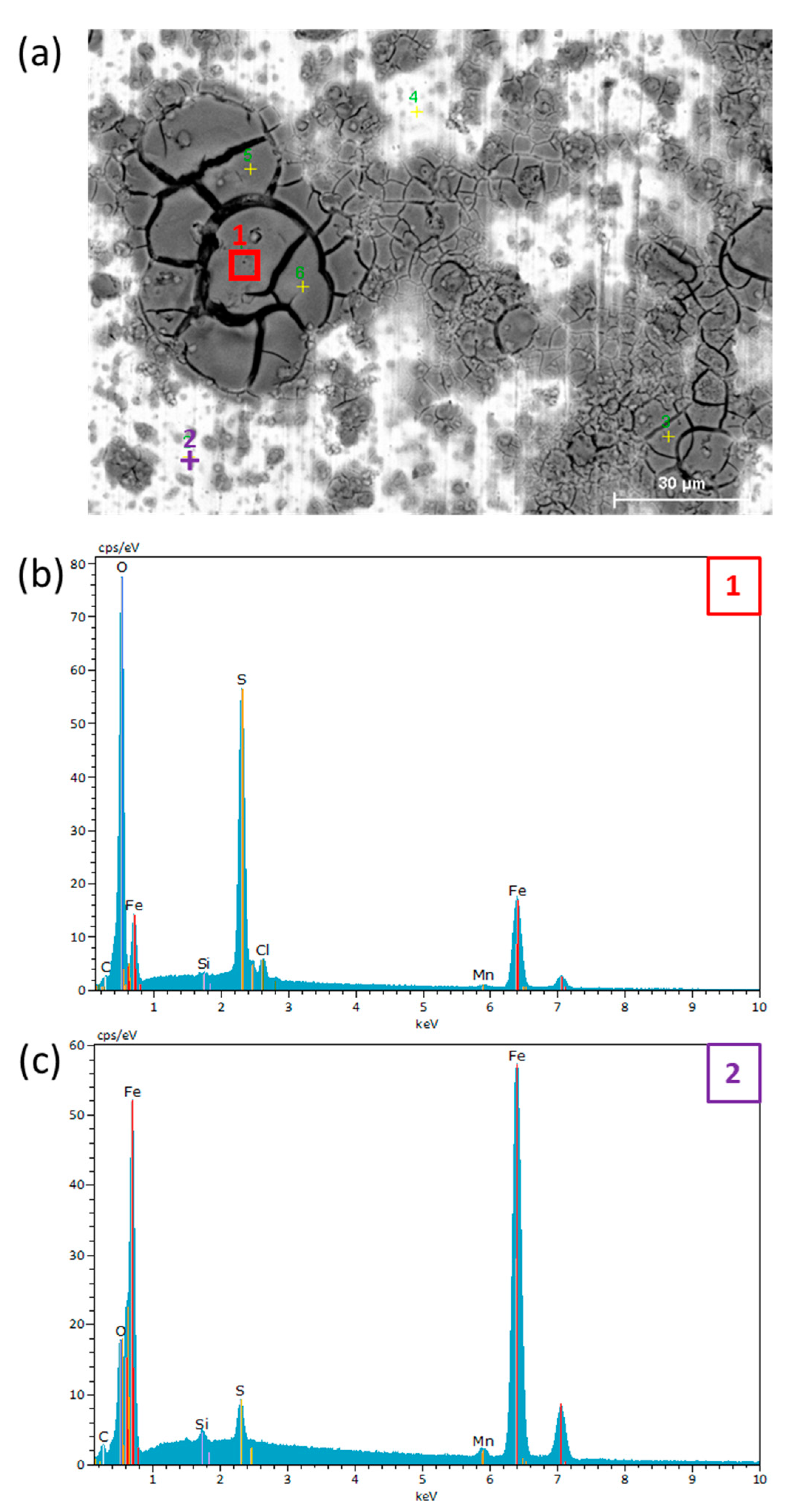
Figure 10.
Backscattered electron (BSE) images displaying focused iron beam (FIB) cross-sectioning of the specimen (X70) with corrosion products and deposited Pt protection layer on top. The thickness of the layer is about 0.2 µm.
Figure 10.
Backscattered electron (BSE) images displaying focused iron beam (FIB) cross-sectioning of the specimen (X70) with corrosion products and deposited Pt protection layer on top. The thickness of the layer is about 0.2 µm.
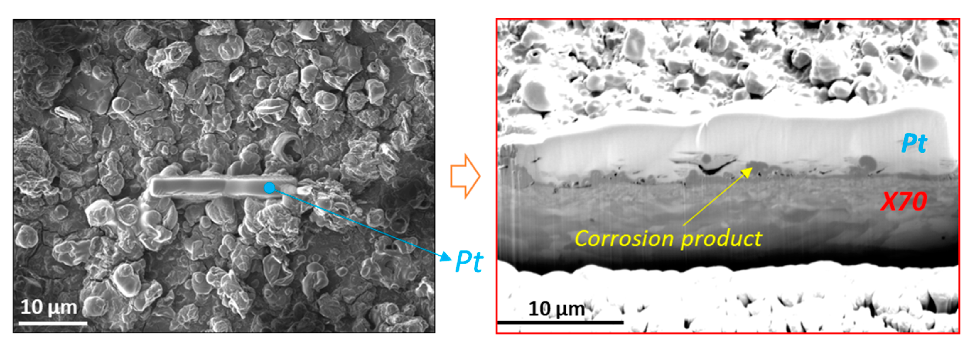
Figure 11.
Figure 11. Line scan of a FIB lamella taken from a corroded specimen from an in-situ EDXRD experiment. (a) Overview of the examined surface showing the sectioned position. (b–d) show the magnification of the analyzed surface/line. (e) Elemental distribution along the line scan, starting from the inside metal substrate (LG2).
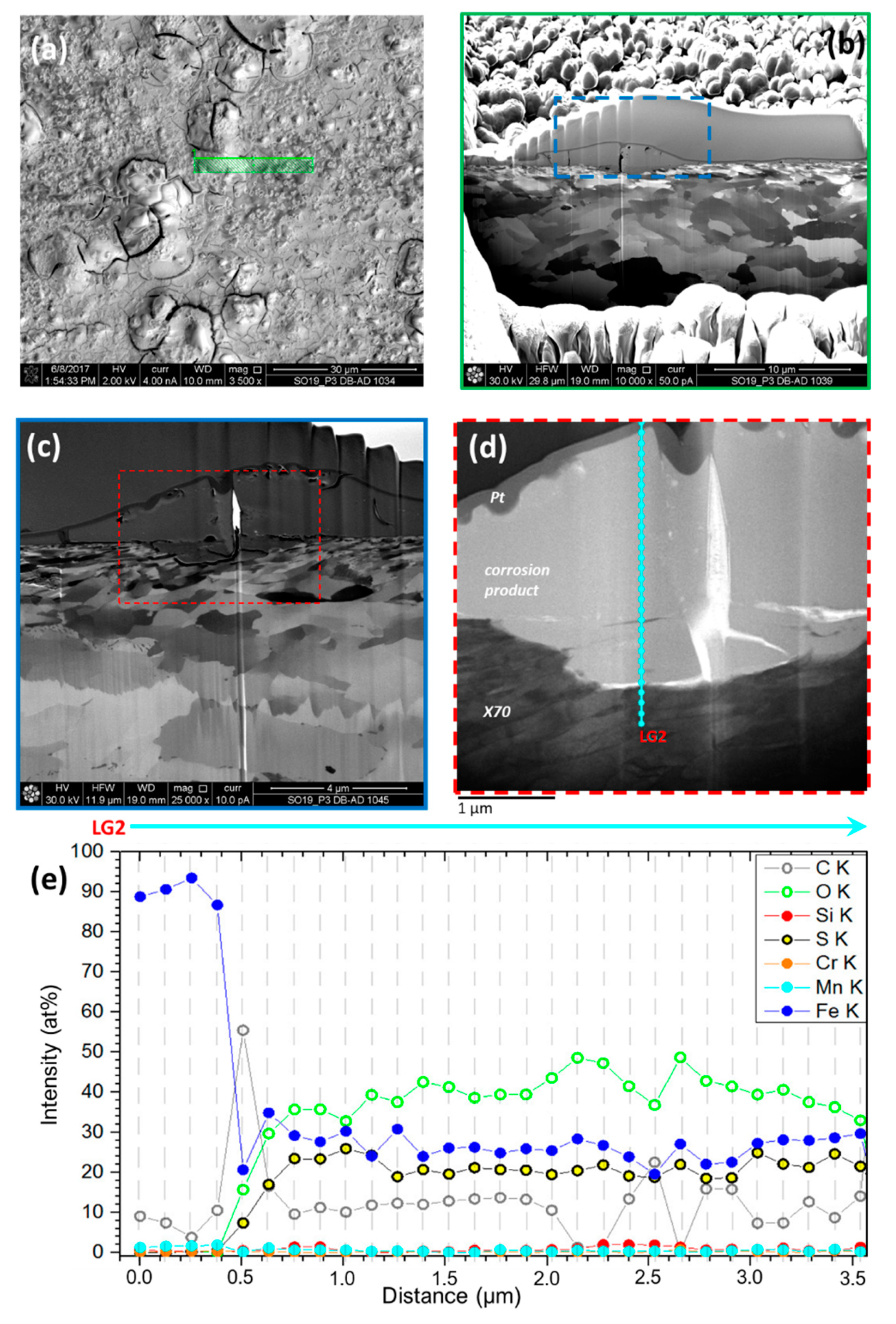
Figure 12.
Left: High-resolution BSE image (bright field) by STEM of the position in Figure 11d. Within the homogeneously colored corrosion layer are spotted areas with brighter or darker contrast. These are associated with a slightly different chemical composition compared to the main part of the corrosion layer. Right: Nanobeam diffraction pattern by STEM of the corrosion product (top) and X70 (bottom). For X70, sharp reflexes are visible, while the pattern of the corrosion layer is small and blurred, implying a ring structure.

Figure 13.
Raman spectrum of the corrosion layer (at the bottom) and two globular structures on top of the corrosion layer (middle and upper graph). Meanwhile, the layer is a complex of different water-bearing iron sulfates or nitrates; the spectra of the structures can be assigned clearly to Rozenite (FeSO4·4 H2O) and Hematite (α-Fe2O3), respectively.
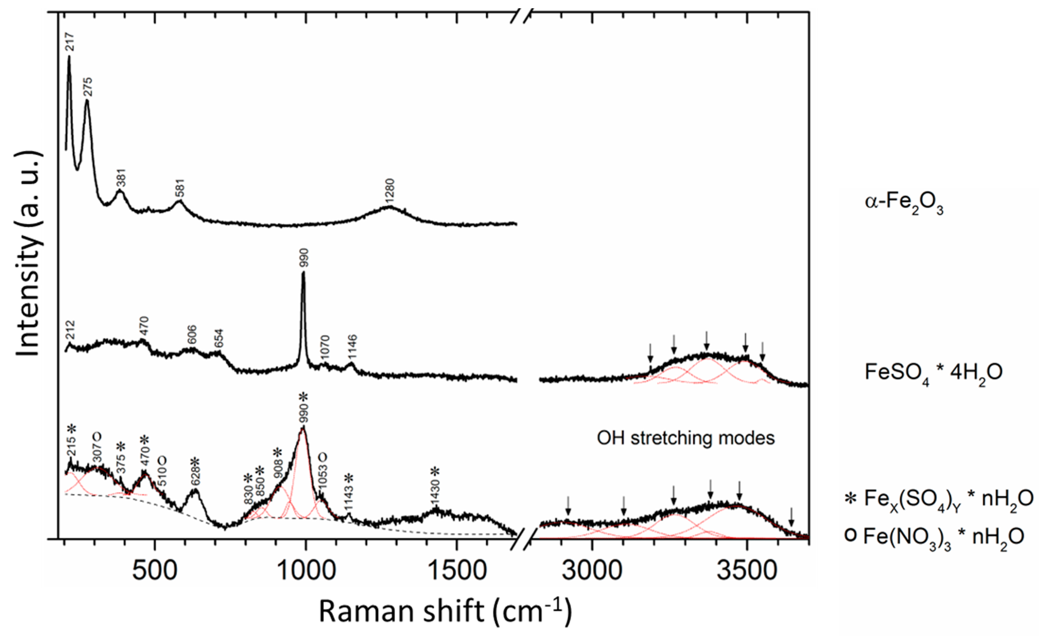
Figure 14.
XRD pattern of the specimen before (a) and after the in-situ corrosion experiment (b). In the upper part of the graphic, an X-ray diffractogram of a long-term corrosion experiment with an increased water content (c) is displayed. The measurements were performed in the grazing incidence mode (GIXRD) at ω = 1, Δt = 15 s/step and Δ2Θ = 0.01 using a Co tube. The sharp reflex at 2Θ = 52.36 belongs to α-Fe, which is related to the specimen (X70). The diffractogram of the in-situ corrosion experiment displays no crystalline phase in the corrosion layer. In contrast, the long-term (168h) experiment demonstrates a high crystallinity for the corrosion products. Those are built up proportionally by Metahohmannite Fe2[O(SO4)3]·4H2O (*), Rozenite FeSO4·4H2O (+), Lausenite Fe2(SO4)3·4H2O (^), Mikasaite Fe2(SO4)3 (#), Hohmannite Fe2[O(SO4)3]·8H2O (o) and Ferricopiapite Fe5(SO4)6(OH)2·20 H2O (~).
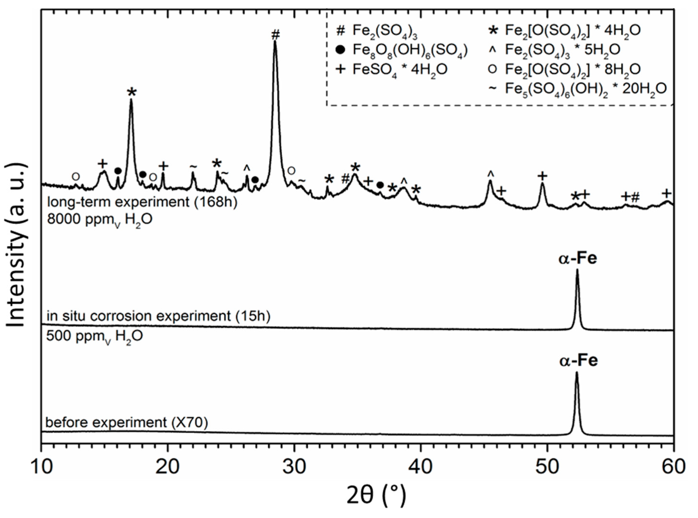
Figure 15.
Reference areas (2 × 2 mm2) of the specimen surface before (a) and after (b) the corrosion experiment. Both images show parallel marks caused by grinding prior to the experiment to homogenize and activate the specimen surface. Attributed to the grinding marks, morphological differences of around 0.5 µm can be observed by a color-coded scale. In addition, image (b) shows shallow pits exhibiting lateral dimensions up to 120 × 50 µm and depths up to 10 µm. The pits are bound to grinding marks and parallel oriented to these.

Table 1.
Chemical composition with major elements of the investigated pipeline steel (X70) *.
| Element | C | Mn | Si | P | S | Cr | Ni |
|---|---|---|---|---|---|---|---|
| % by mass | 0.16 | 1.70 | 0.45 | 0.02 | 0.02 | 0.03 | 0.05 |
* Fe-balanced.
Table 2.
List of the energy of emission lines (keV) and onset time (min) corresponding to the corrosion phases generated in the time-resolved in-situ experiment at BESSY II (Figure 7b–d).
Table 2.
List of the energy of emission lines (keV) and onset time (min) corresponding to the corrosion phases generated in the time-resolved in-situ experiment at BESSY II (Figure 7b–d).
| Emission Line (keV) | Lattice Parameter (Å) | Onset (min) | Phase Formula (hkl) | ||
|---|---|---|---|---|---|
| 20.10 | 5.993 | ~360 | Metahohmannite | Fe2(SO4)2O·4 H2O | (110) |
| 26.35 | 4.500 | ~240 | Rozenite | FeSO4·4 H2O | (111) |
| 31.81 | 3.757 | ~360 | Metahohmannite | Fe2(SO4)2O·4 H2O | (12–1) |
| 36.35 | 3.204 | ~150 | Lausenite | Fe2(SO4)3·5 H2O | (30–1) |
| 40.18 | 2.946 | ~360 | Metahohmannite | Fe2(SO4)2O·4 H2O | (211) |
© 2020 by the authors. Licensee MDPI, Basel, Switzerland. This article is an open access article distributed under the terms and conditions of the Creative Commons Attribution (CC BY) license (http://creativecommons.org/licenses/by/4.0/).
Share and Cite
MDPI and ACS Style
Kratzig, A.; Quynh Hoa, L.; Bettge, D.; Menneken, M.; Bäßler, R. Early Stage of Corrosion Formation on Pipeline Steel X70 Under Oxyfuel Atmosphere at Low Temperature. Processes 2020, 8, 421. https://doi.org/10.3390/pr8040421
AMA Style
Kratzig A, Quynh Hoa L, Bettge D, Menneken M, Bäßler R. Early Stage of Corrosion Formation on Pipeline Steel X70 Under Oxyfuel Atmosphere at Low Temperature. Processes. 2020; 8(4):421. https://doi.org/10.3390/pr8040421
Chicago/Turabian StyleKratzig, Andreas, Le Quynh Hoa, Dirk Bettge, Martina Menneken, and Ralph Bäßler. 2020. "Early Stage of Corrosion Formation on Pipeline Steel X70 Under Oxyfuel Atmosphere at Low Temperature" Processes 8, no. 4: 421. https://doi.org/10.3390/pr8040421
Note that from the first issue of 2016, this journal uses article numbers instead of page numbers. See further details here.