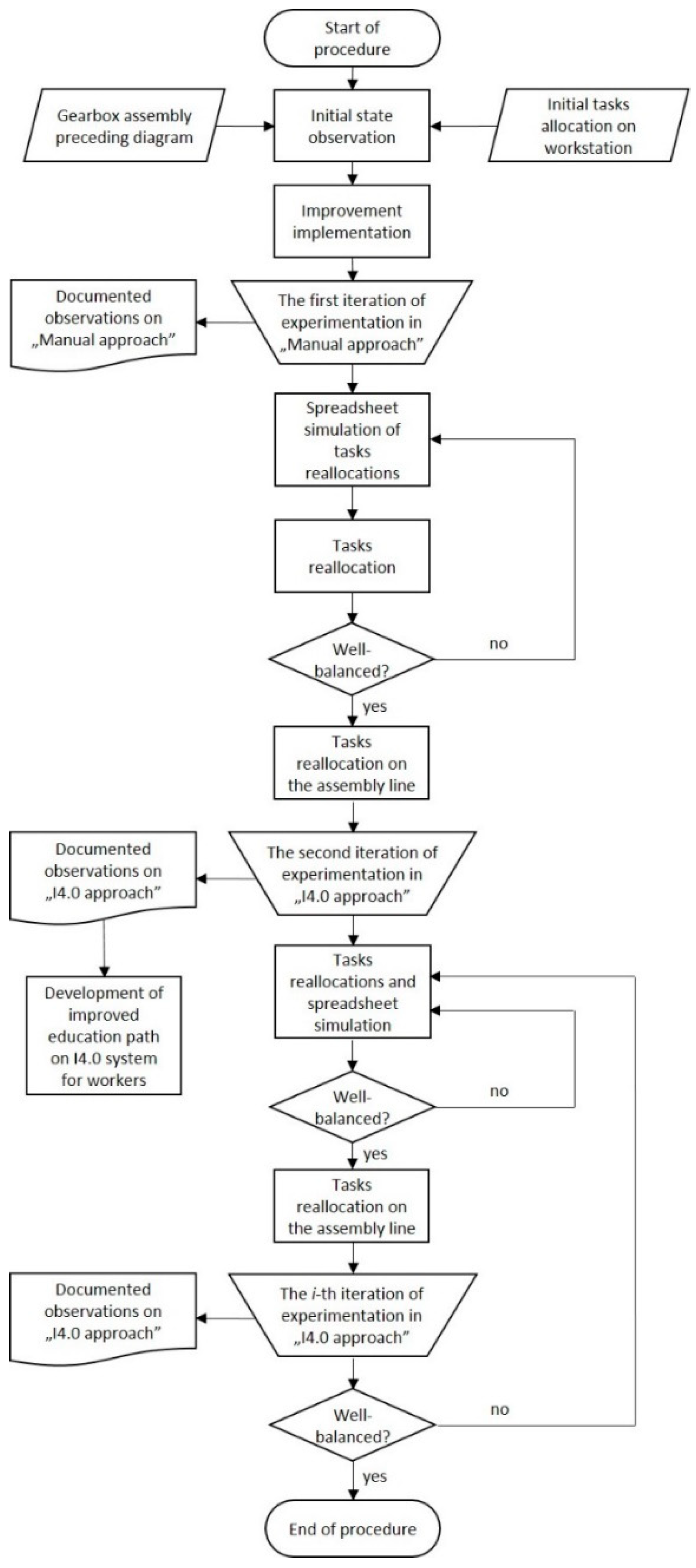
2.3.1. Manual Approach for the First Iteration
The starting point of the procedure is the observation of the current state presented in previous work [
41]. The process times and process times standard deviations are shown in
Table 1.
Prior to the first iteration of assembly line balancing procedure, improvements on setup presented in [
41] are introduced. Excessive workloads on WS1, WS2, WS4, and WS5, compared to WS3, are attempted to be solved by the introduction of electric screwdrivers and improved instructions to workers. WS5 is additionally equipped with gravity conveyer to relief worker from lifting heavy upper casing to compensate time needed for 11 new parts to be assembled on that WS. WS3, as the WS with the lowest process time, is significantly influenced by the introduction of low-volume/high-variety production, in terms of many different parts to be inserted according to product type. That should increase the process time on WS3. Therefore, it is expected that the assembly line will be better balanced with the implementation of improvements and changes in a number of parts compared to the case shown in [
41].
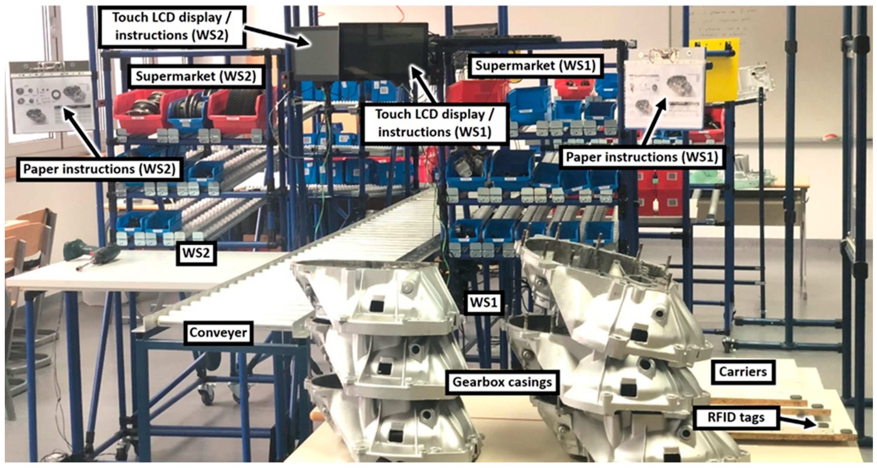
Assembly process with “Manual approach” used information flow on paper sheets and manual data gathering process by analysts. Ten participants are required to perform experimentation run. Five participants are workers, working on five WSs, and another five participants are trained time study analysts, as every WS requires one to achieve realistic process time measurements and additional observations. Analysts’ first task was to recognize feasible assembly steps. The warm-up period prior to experimentation enabled analysts, to define assembly steps, and workers, to achieve the necessary skill in performing assembly. During experimentation run, analysts gathered process times of every individual assembly step. Total process time on every WS was calculated by the summation of assembly steps process times. Additional analysts’ task was to monitor workers’ activities, related to the usage of the production plan and to the usage of available work instructions on paper sheets.
Production plan was available on every WS in the form of paper spreadsheet revealing assembly sequence. Detailed paper instructions, including photographs of parts to be installed, were hanging in sight of workers, on paper sheets. As there was more than one assembly step defined on every WS, and there are differences between types of gearboxes, eight paper sheets in average were available for listing at every WS. The first iteration of experiments was performed with a total of 24 gearboxes assembled.
Method of timing by stop watch, i.e., snap back method [
42] is used for time gathering purpose. Abnormal values during readings are recorded together with its causes of abnormality. Those values can be used in further analysis to improve processes. If those abnormalities occurrences are neglected, process times variations increase abnormally, which do not reflect the real process times [
42]. The simplified method used includes only three causes of abnormality: the problem with tools, denoted as “T,” the problem with parts, denoted as “Z,” and bad material detected, denoted as “M.” Detection of abnormalities and duration of those were important in further considerations for line balancing and for assembly improvement process on every WS.
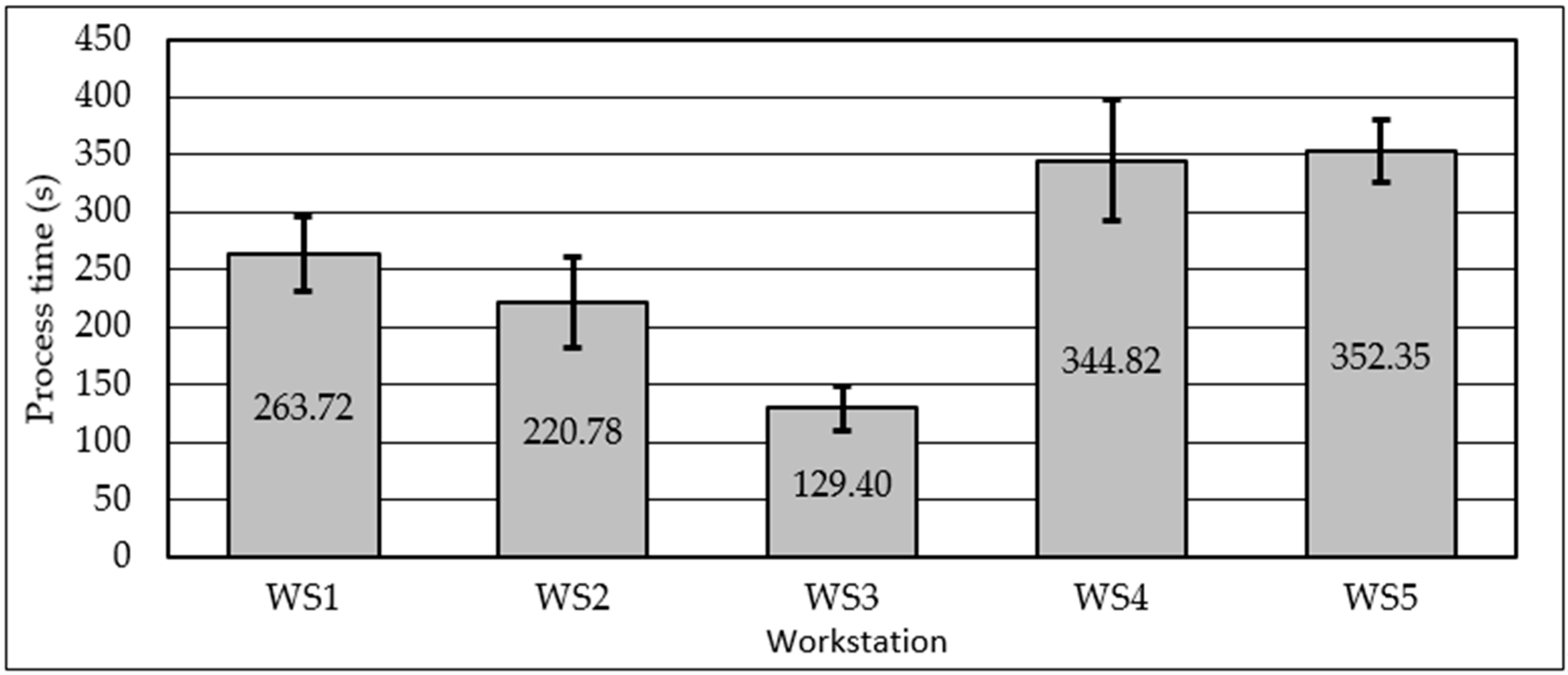
After the first iteration experimentation run, the manually written data on snap back method template were transferred to digital spreadsheet in order to calculate mean and standard deviation of process times automatically.
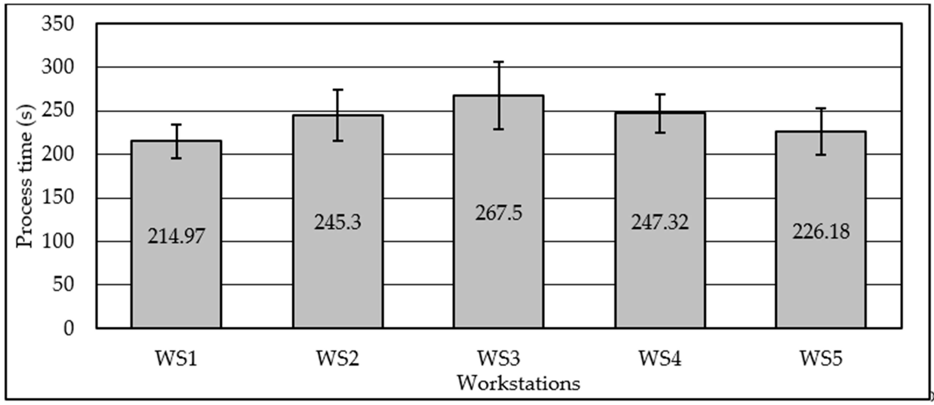
Table 2 shows data gathered for all five WSs. Average process times with error bars presenting standard deviations are shown in
Figure 6.
It can be seen in
Figure 6 that process times vary enormously among WSs. Achieved results showed that workload distribution, as a result of the previous investigation [
41], was not appropriate, although implemented improvements and introduction of product variety were expected to improve work balance among WSs. During observations, another issue disbalancing assembly line was found. It laid in the mutual impact of one WS activity on neighbor WS activity. During assembly, bottleneck occurred on WS5. There are WSs with higher workloads than neighboring WSs (i.e., WS1).” When WS is a bottleneck or have a higher workload, there is a starvation, i.e., lower utilization on succeeding WS, and idle time occurs. During this idle time, i.e., waiting time for the next product, worker can perform some activities and some improvements. Assembly steps are generally planned to be performed when product arrives at WS. However, the activities that can be done in idle time, without the presence of gearbox are: introduction with the following product type, determination of parts location needed for the following product, selection and pull-out of parts from supermarkets and disposition on the worktable, the formation of subassembly on worktable although those are not defined in preceding diagram, etc. Therefore, WS with shorter process time will reduce its process time even more, as it can work in parallel with preceding WS. The analyst starts to gather process time as instructed, at the moment when gearbox arrives on WS. Additional activities, done prior to gearbox arrival are partly recorded, but cannot be assigned easily to some activity or to some product. It is the case especially if preparation and improvement is done to next few products. So, this data cannot be analyzed or used subsequently in the line balancing process.
This phenomenon is neglected in manual assembly lines where the arrival of the product on WS is the trigger for the start of process time gathering. Human workers are more flexible and intelligent then programmed robots, so the human worker will adapt to the situation and improve their activities. Although standard work procedure is deployed for all WSs, it is in human nature to improve processes and speed it up if found possible. This is making assembly line even worse balanced in this case (
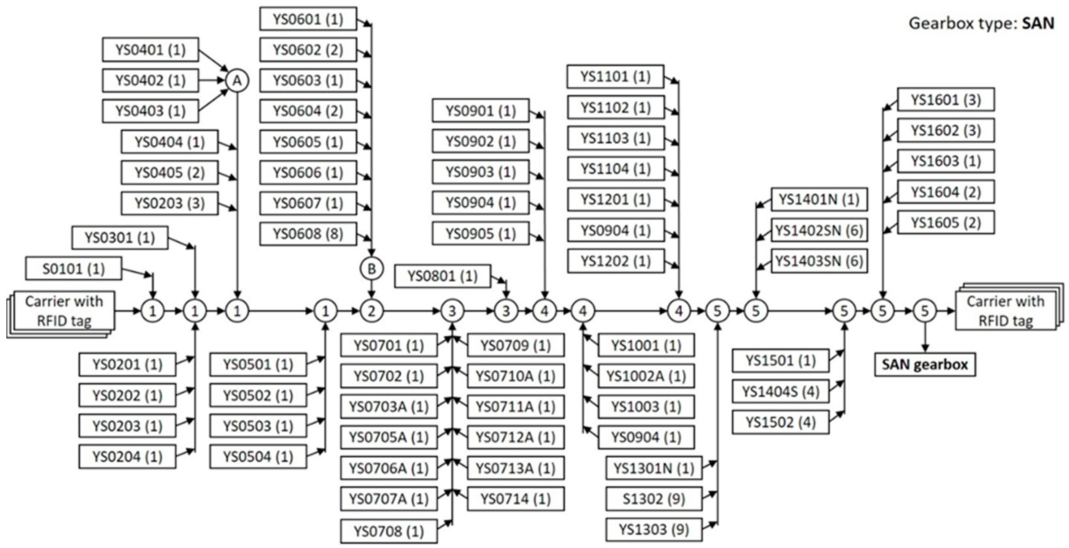
Figure 6). By assembly process observation, it was found that worker on WS3 utilized idle time in collecting parts YS0701 to YS0714 on the worktable, in disposition appropriate for fast installing when gearbox arrived on WS3. In later experimentation period, parts YS0701 to YS0714 were assembled in subassembly on the worktable and inserted in gearbox in a very short time (about 4 s needed). This reorganization and improvements initiated by the worker on WS3 enabled even higher disbalance than found in previous research [
41].
A total of 22 assembly steps were recognized and individual process times were collected. Those assembly steps were used for reallocation purposes in following balancing processes. The commonly used balancing method, largest candidate rule (LCR) [
43], was used. The goal was to find the minimum number of WSs for defined customer overall cycle time, i.e., assembly line overall cycle time. In the presented case study, the number of WSs was predefined, by layout constraints, as five. The objective was minimizing the cycle time when the number of stations was fixed, and it was considered as “Type 2” problem, according to [
44]. Therefore, assembly steps were reallocated only among existing WSs, taking the preceding diagram into consideration. Prior to that activity, the total assembly process time was used in order to the get ideal overall cycle time,
, after 1 iteration according to the Equation (1):
where
NWS is the number of workstations.
Ideal overall cycle time is the process time goal for every WS. As the total number of WSs is limited to five, achievable overall cycle time found in the bottleneck process is higher than the ideal overall cycle time. Therefore, the balancing process is performed by spreadsheet simulation according to LCR in the sufficient number of iterations. As minimum assembly step duration was 8.12 s, rounded increase of 5 s in every iteration on the ideal overall cycle time was appropriate. In iteration when assembly line overall cycle time was increased to 285 s, all assembly steps were allocated in only five WSs and that was considered as successfully performed balancing process. Only four assembly steps reallocations were found.
Table 3 presents reallocation of assembly steps.
It was found that the optimal distribution resulted with the highest process time (bottleneck process time) of 28,295 s on WS2. Therefore, WS2 was expected to be a bottleneck process in the second experimentation iteration.
The expected work distribution was optimal when using 22 assembly steps. However, it is still not perfectly balanced, as shown in
Table 3. The assembly step represented a part or a group of parts to be inserted in the gearbox to build some feature or entirety. Further fragmentation of assembly steps was not appropriate, as fragmentation generally increased the number of different parts on supermarkets and the complexity of the assembly process on most WSs. For example, switching installation and screwing process for five sets (from total nine) of washers and nuts (YS1303 and S1302) from WS4 to WS5 will improve balancing to some extent. However, two more part boxes should be installed in the supermarket of WS5, and clear guidance to install only four sets of washers and nuts on WS4 should be emphasized. Problems that also can be expected comprise unnecessary doubling of tools, missing to install some washers and nuts, missing to tighten all nuts to final torque, more intensive information flow resulting with an increased number of instruction pages, etc. Therefore, only a total of 22 assembly steps remained for reallocation purposes during the balancing process.
Table 3 shows predicted process times on WSs according to spreadsheet simulation. When reallocating assembly steps to another WS, its process time could be changed due to more reasons. The WS and supermarket layout and the instructions were changed. Level of gearbox completion could also be changed, which, therefore, changing accessibility when installing parts, thus increasing or reducing the speed of insertion. Therefore, the second iteration of experimentation should validate spreadsheet simulation results.
After the reorganization of the assembly line, the introduction of I4.0 related equipment and update of instructions pages, the second iteration of experimentation run took place. In this experimentation run, “I4.0 approach” was used for information flow and data gathering process.
2.3.2. I4.0 Approach for the Second Iteration
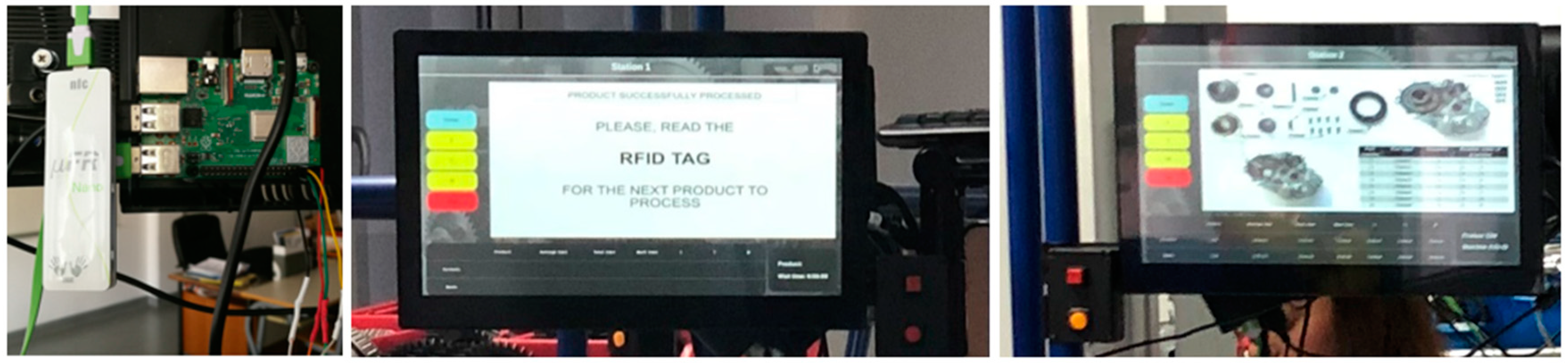
For transportation of the gearboxes along the assembly line, the carriers were used. Each carrier had glued passive RFID tag that carried the information which was not related to any of gearboxes. RFID system installed on every WS was controlled by Raspberry Pi 3B+, manufactured by Sony UK Technology Centre, Pencoed, UK, (RPi) server with Raspbian GNU/Linux 9.6, manufactured by Raspberry Pi Foundation, Cambridge, UK, over a Wi-Fi connection. On every WS, there was Raspberry Pi 3B+ microcomputer with touch LCD display and µFR Nano RFID reader with an antenna. The system was programmed in “Node.js” version 11.6.0, manufactured by OpenJS Foundation, Joyent, Inc., San Francisco, United States of America, with execution environment using “Express.js”, framework, manufactured by OpenJS Foundation, Joyent, Inc., San Francisco, United States of America. JavaScript, manufactured by OpenJS Foundation, Joyent, Inc., San Francisco, United States of America was used with “HTML” supporting “CSS”, manufactured by Tim Berners-Lee contractor of Organisation européenne pour la recherche nucléaire (CERN), Geneva, Switzerland, for the graphical user interface. Additional push buttons, for process completion signal and for the listing of instructions were installed in the separate electronic box positioned near to LCD display. The touch LCD display displayed the instructions to workers, same to those found on paper sheets. Another functionality found on display, besides time counters, was the production plan table line defined by the type of product to be assembled. There was another table line with following product to be assembled and field that revealed wait time, if the product was already completed on preceding workstation.
Additional buttons, namely, T, Z, M, and Normal gave the possibility to worker to switch counters if the process was abnormal and then switching back to normal when the issue was solved. With the STOP button, counters could be stopped and resumed at any moment, if there was a need for leaving the working place.
The server read the regularly updated spreadsheet document which was the production plan. When an RFID tag passed by the antenna on WS1, the server sent information which product was to be assembled and assigned text string from RFID tag to the product. By tracking this RFID tag, the server monitored the location and gathered the process times and abnormality times on every WS for that particular product. When the product was completed on WS5, server released RFID tag information and calculated the total lead time for the specific product. The carrier with the RFID tag could be used again for another gearbox, without any action required. All collected data about the product assembling was available on the server for postprocessing purposes. The main components of I4.0 RFID system and display appearances are shown in
Figure 7.
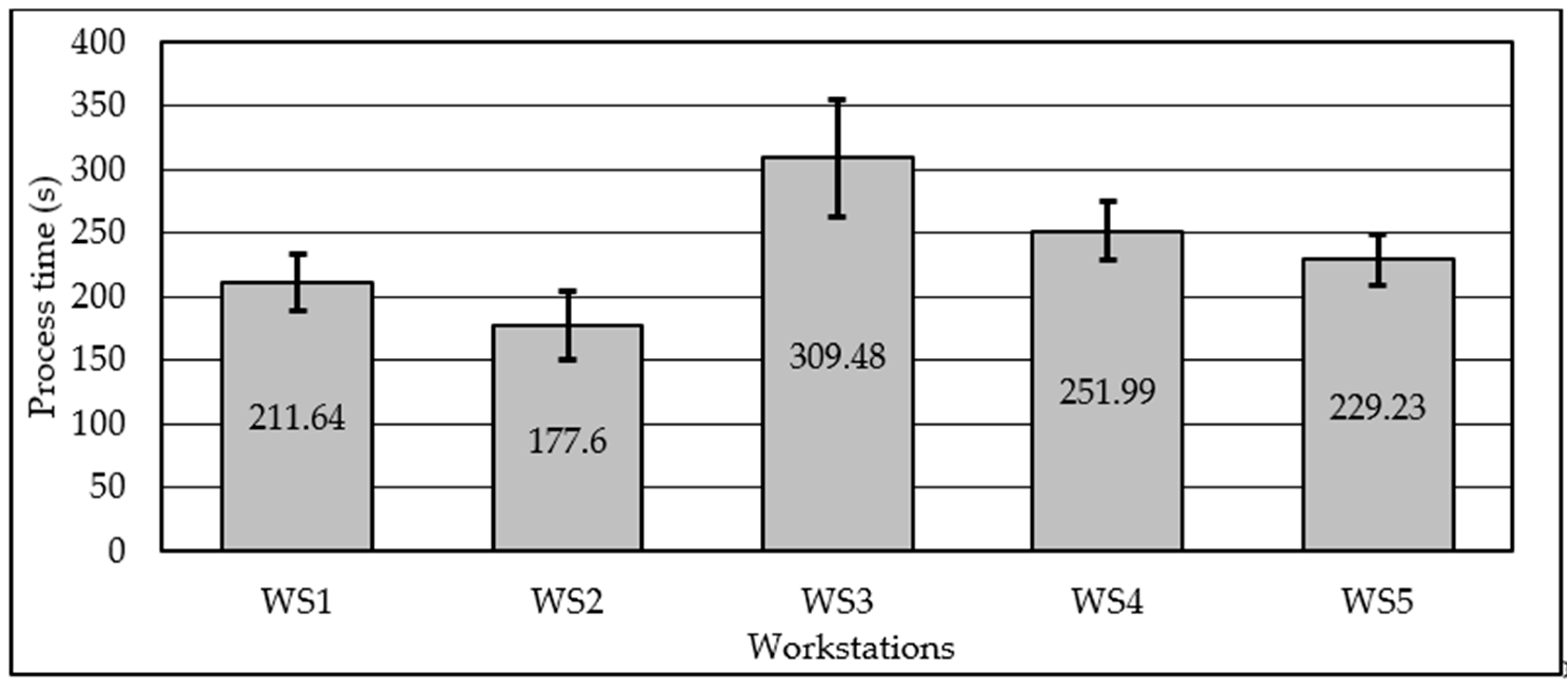
Only five workers were necessary for performing experimentation in the second iteration, as I4.0 related equipment introduction aims to replace analysts. Nevertheless, analysts were present to gather data about workers’ behavior on performing activities according to deployed procedures and instructions. Control stopwatches were used by analysts, to gather cycle times on WS, although “I4.0 approach” did not require analysts with stopwatches. Total 24 gearboxes were assembled. The data gathered by I4.0 related equipment are listed in
Table 4. Average process times with error bars presenting standard deviations are shown in
Figure 8.
The I4.0 system was functioning faultlessly. However, the workers did some mistakes using it, so a total of 14 readings were useless (from total 120). The control stopwatches data were used instead to gather process times.
The errors that workers did are listed according to their number of appearances:
Worker forgot to complete the process when finished by pressing pushbutton (four appearances).
Worker did unsuccessful RFID reading by reading the RFID tag too fast (three appearances).
Worker did not use process abnormality counters (Z, T, and M) and therefore, normal process time was increased abnormally (three appearances).
Worker did not check all pages of instruction, and therefore, inserted wrong parts (two appearances).
Worker did not check the production plan, then assembled the wrong type of gearbox (one appearance).
Worker completed the process by pushbutton immediately after RFID reading (one appearance).
I4.0 system functionality was not compromised at any moment, but workers had to be more focused on display and to check regularly if content shown was aligned to expected. This was emphasized in moments where information flow from human to RFID system take part, i.e., in reading the RFID tag and completing the process with the pushbutton.
As shown in
Table 4, the worker on WS3 had many more issues during the assembly process than in the first iteration (Z and T abnormalities readings). The reallocation of assembly steps initiated a new approach in gear lever mechanism assembly. In two moments of the assembly activities, special skills were requested from worker to insert parts while having very small tolerances for insertion. This very complex activity had a high assembly process time and standard deviation. WS3, therefore, became the bottleneck. As a worker on bottleneck process (WS3) do not have idle time, activities performed in the first iteration by the worker on WS3 did not took part, which was another reason why process time on WS3 was considerably longer than predicted in
Table 3. Due to the bottleneck process on WS3, unfinished gearboxes occupied conveyor, which, therefore, enable some idle time on WS1 and WS2. This idle time was thus used for improvements by workers on WS1 and WS2, which reduced respective processes times.
Prior to the third iteration of experimentation, the new observations by analysts should be included. Assembly steps process times on WS1 to WS3 were found different from those gained in the first iteration, due to aforementioned reasons. Nevertheless, the assembly steps in WS4 and WS5 showed negligible differences in process times. Lower accessibility and more complex manipulation needed on WS3 changed assembly steps times significantly compared to those gained in the first iteration. There was a noticeable reduction in total processing time, in comparison to total processing time calculated in the first iteration, which led to reduced ideal overall cycle time (Equation (2)).
For the second iteration, the same spreadsheet simulation approach was used. In simulated iteration when assembly line overall cycle time was increased to 255 s, all assembly steps were allocated in only five WSs and was considered as successfully performed balancing process. It was found that only one reallocation of assembly step had to be performed (
Table 5).
After the reorganization of the assembly line and update of instructions pages, the third iteration of experimentation run took place. Workers were trained intensively about how the RFID system works and how it will respond in some boundary conditions.


