Application of Systems Engineering Principles and Techniques in Biological Big Data Analytics: A Review


Abstract
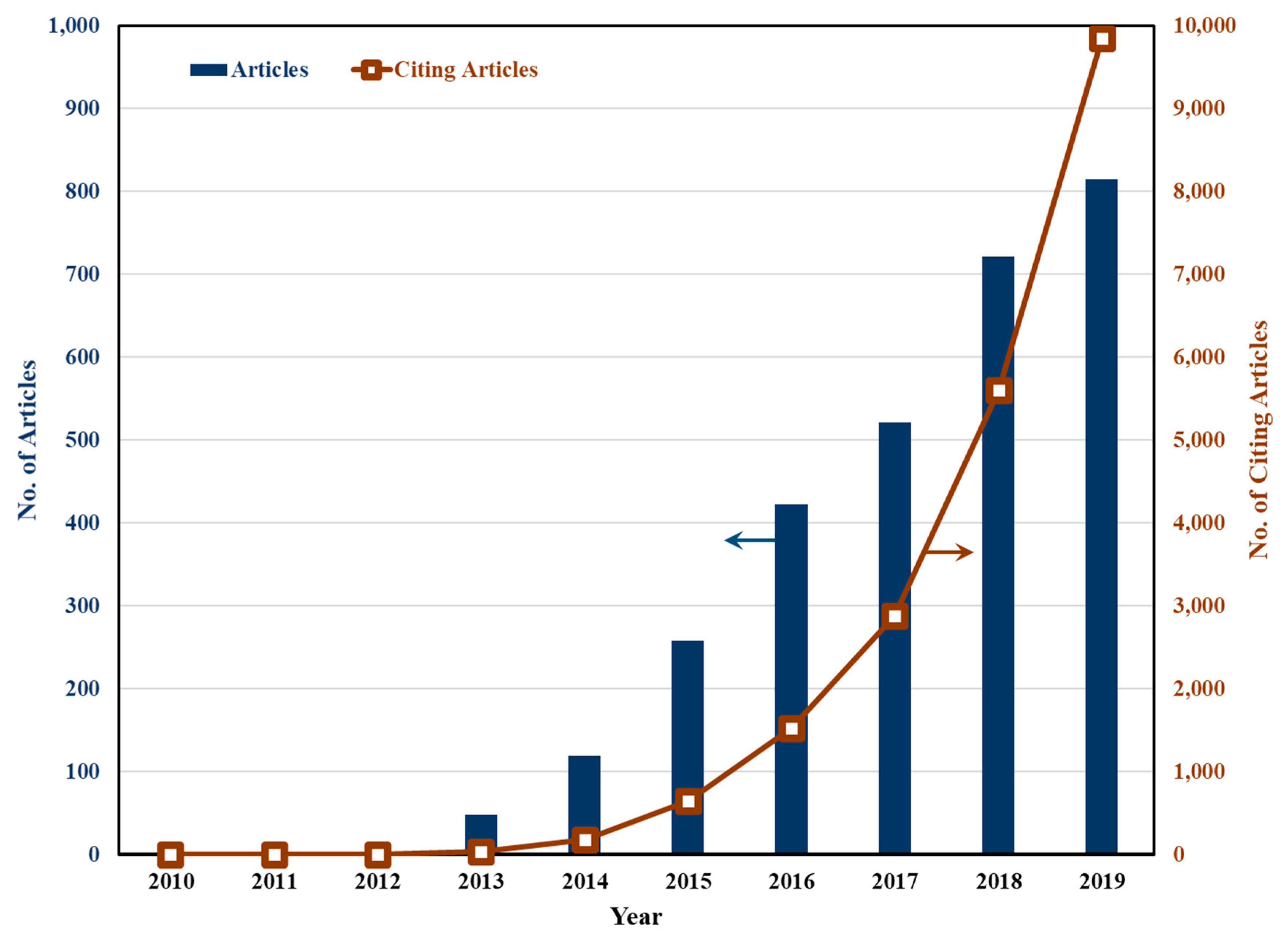
:1. Introduction
2. Principle of Parsimony in Addressing Overfitting
2.1. Checking for Overfitting
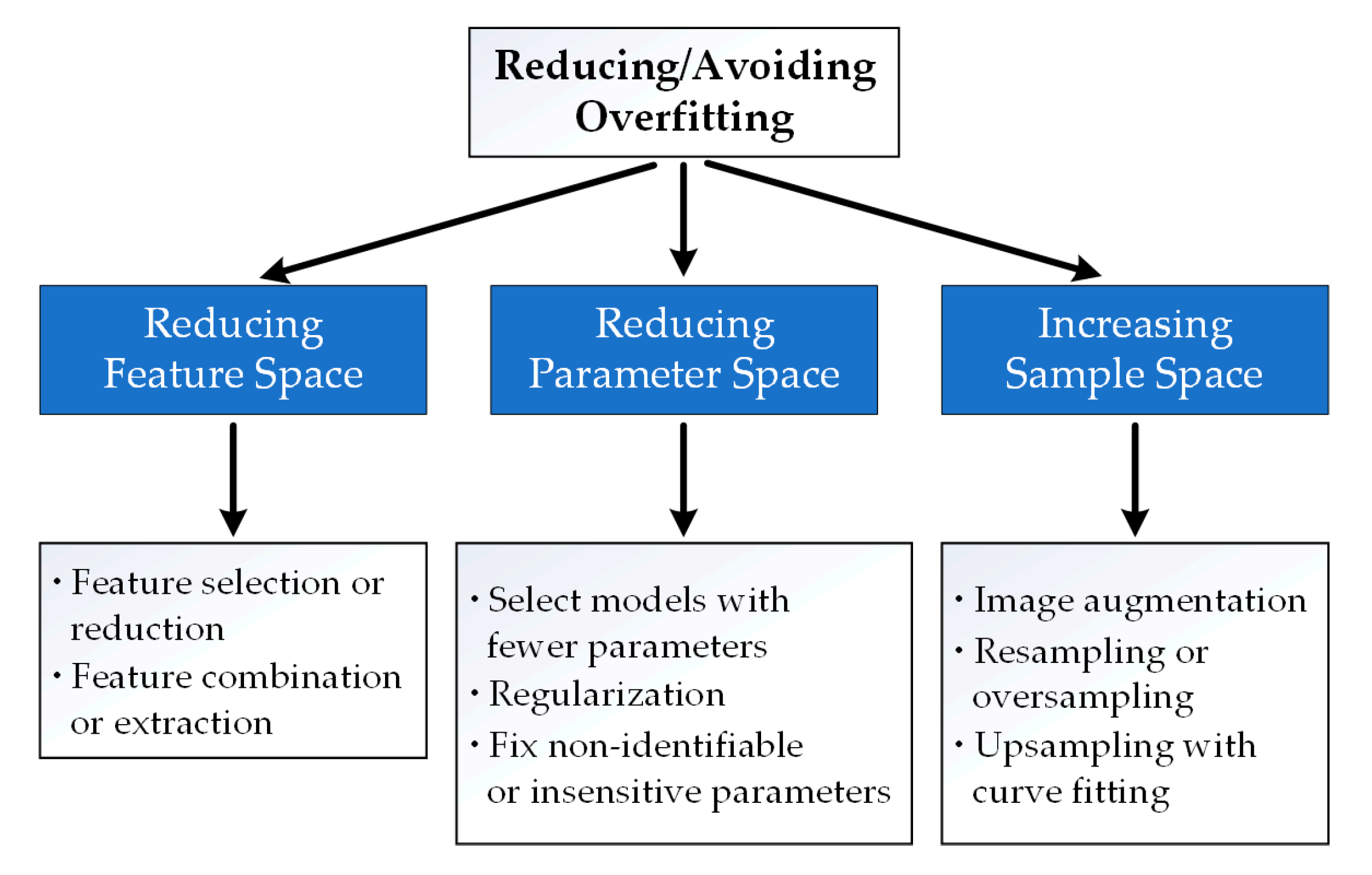
2.2. Reducing or Avoiding Overfitting
2.2.1. Reducing Feature Space
Feature Selection or Reduction
Feature Combination or Extraction
2.2.2. Reducing Parameter Space
Selecting a Model with a Small Number of Parameters
Regularization
Model Parameter Identifiability Analysis and Sensitivity Analysis
2.2.3. Increasing Sample Space
2.3. Summary and Discussion
3. Dynamic Analysis of Biological Data
3.1. Dynamic Analysis of Genomics Data
3.2. Dynamic Metabolic Flux Analysis
3.3. Dynamic Analysis of Signal Transduction Networks
3.4. Integrated Dynamic Analysis of Multi-Omics Data
3.5. Other Applications of Dynamic Data Analysis
3.6. Summary and Discussion
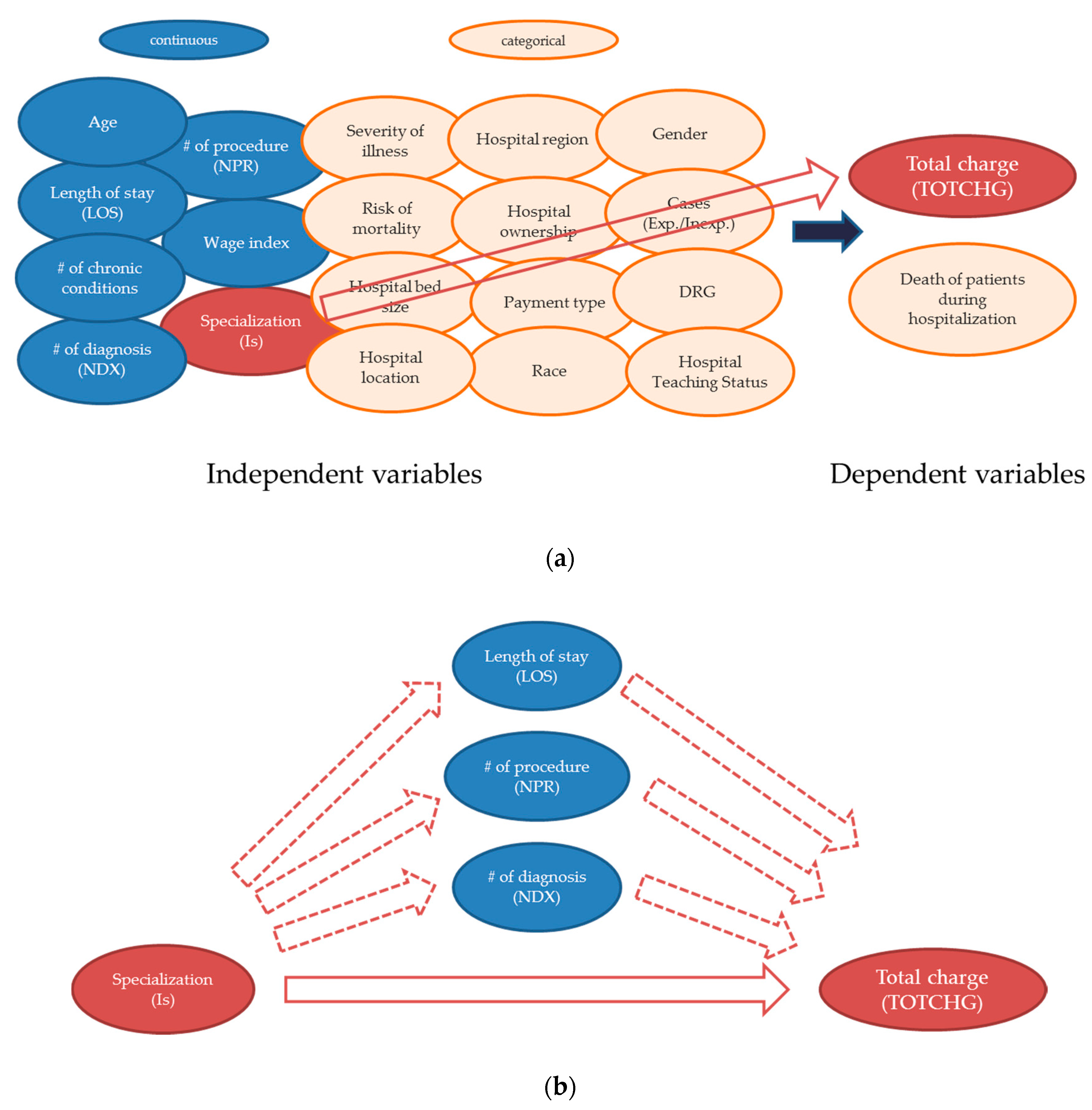
4. The Role of Domain Knowledge in Biological Data Analytics
4.1. Knowledge Matching vs. Point Matching for Model Validation
4.2. Knowledge-Guided Unsupervised Learning
4.3. Knowledge-Guided Supervised Learning
4.4. Knowledge-Guided Feature Engineering and Feature Selection
4.5. Summary and Discussion
5. Conclusions
Author Contributions
Funding
Acknowledgments
Conflicts of Interest
References
- Zikopoulos, P.; Eaton, C. Understanding Big Data: Analytics for Enterprise Class Hadoop and Streaming Data; McGraw-Hill Osborne Media: New York, NY, USA, 2011. [Google Scholar]
- Zikopoulos, P.C.; Deroos, D.; Parasuraman, K. Harness the Power of Big Data: The IBM Big Data Platform; McGraw-Hill: New York, NY, USA, 2013; ISBN 0071808183. [Google Scholar]
- Yang, L.T.; Chen, J. Special Issue on Scalable Computing for Big Data. Big Data Res. 2014, 100, 2–3. [Google Scholar] [CrossRef]
- Liang, T.-P.; Guo, X.; Shen, K. Special Issue: Big data analytics for business intelligence. Expert Syst. Appl. 2018, 111, 1. [Google Scholar] [CrossRef]
- Martínez–Álvarez, F.; Morales–Esteban, A. Big data and natural disasters: New approaches for spatial and temporal massive data analysis. Comput. Geosci. 2019, 129, 38–39. [Google Scholar] [CrossRef]
- Bassi, S. A primer on python for life science researchers. PLoS Comput. Biol. 2007, 3, e199. [Google Scholar] [CrossRef] [PubMed]
- Ekmekci, B.; McAnany, C.E.; Mura, C. An introduction to programming for bioscientists: A Python-based primer. PLoS Comput. Biol. 2016, 12, e1004867. [Google Scholar] [CrossRef] [PubMed] [Green Version]
- Charalampopoulos, I. The R Language as a Tool for Biometeorological Research. Atmosphere 2020, 11, 682. [Google Scholar] [CrossRef]
- Peng, R.D. Reproducible research and biostatistics. Biostatistics 2009, 10, 405–408. [Google Scholar] [CrossRef]
- Peng, R.D. Reproducible research in computational science. Science (80-) 2011, 334, 1226–1227. [Google Scholar] [CrossRef] [Green Version]
- Stodden, V. Reproducible research: Tools and strategies for scientific computing. Comput. Sci. Eng. 2012, 14, 11–12. [Google Scholar] [CrossRef] [Green Version]
- Mittelstadt, B.D.; Floridi, L. The ethics of big data: Current and foreseeable issues in biomedical contexts. Sci. Eng. Ethics 2016, 22, 303–341. [Google Scholar] [CrossRef]
- Raghupathi, W.; Raghupathi, V. Big data analytics in healthcare: Promise and potential. Heal. Inf. Sci. Syst. 2014, 2, 3. [Google Scholar] [CrossRef]
- Feldman, B.; Martin, E.M.; Skotnes, T. Big data in healthcare hype and hope. Dr. Bonnie 360 2012, 122–125. [Google Scholar]
- Mehta, N.; Pandit, A. Concurrence of big data analytics and healthcare: A systematic review. Int. J. Med. Inform. 2018, 114, 57–65. [Google Scholar] [CrossRef]
- Senthilkumar, S.A.; Rai, B.K.; Meshram, A.A.; Gunasekaran, A.; Chandrakumarmangalam, S. Big data in healthcare management: A review of literature. Am. J. Theor. Appl. Bus. 2018, 4, 57–69. [Google Scholar]
- Alyass, A.; Turcotte, M.; Meyre, D. From big data analysis to personalized medicine for all: Challenges and opportunities. BMC Med. Genomics 2015, 8, 33. [Google Scholar] [CrossRef] [Green Version]
- Luo, J.; Wu, M.; Gopukumar, D.; Zhao, Y. Big data application in biomedical research and health care: A literature review. Biomed. Inform. Insights 2016, 8, BII-S31559. [Google Scholar] [CrossRef] [Green Version]
- Alonso, S.G.; de la Torre Diez, I.; Rodrigues, J.J.P.C.; Hamrioui, S.; Lopez-Coronado, M. A systematic review of techniques and sources of big data in the healthcare sector. J. Med. Syst. 2017, 41, 183. [Google Scholar] [CrossRef] [PubMed]
- Herland, M.; Khoshgoftaar, T.M.; Wald, R. A review of data mining using big data in health informatics. J. Big Data 2014, 1, 1–35. [Google Scholar] [CrossRef] [Green Version]
- Andrew, C.; Heegaard, E.; Kirk, P.M.; Bässler, C.; Heilmann-Clausen, J.; Krisai-Greilhuber, I.; Kuyper, T.W.; Senn-Irlet, B.; Büntgen, U.; Diez, J. Big data integration: Pan-European fungal species observations’ assembly for addressing contemporary questions in ecology and global change biology. Fungal Biol. Rev. 2017, 31, 88–98. [Google Scholar] [CrossRef]
- Heart, T.; Ben-Assuli, O.; Shabtai, I. A review of PHR, EMR and EHR integration: A more personalized healthcare and public health policy. Heal. Policy Technol. 2017, 6, 20–25. [Google Scholar] [CrossRef]
- Ritchie, M.D.; Holzinger, E.R.; Li, R.; Pendergrass, S.A.; Kim, D. Methods of integrating data to uncover genotype–phenotype interactions. Nat. Rev. Genet. 2015, 16, 85–97. [Google Scholar] [CrossRef]
- Tomar, D.; Agarwal, S. A survey on Data Mining approaches for Healthcare. Int. J. Bio-Sci. Bio-Technol. 2013, 5, 241–266. [Google Scholar] [CrossRef]
- Yoo, I.; Alafaireet, P.; Marinov, M.; Pena-Hernandez, K.; Gopidi, R.; Chang, J.-F.; Hua, L. Data mining in healthcare and biomedicine: A survey of the literature. J. Med. Syst. 2012, 36, 2431–2448. [Google Scholar] [CrossRef] [PubMed]
- Shukla, D.P.; Patel, S.B.; Sen, A.K. A literature review in health informatics using data mining techniques. Int. J. Softw. Hardw. Res. Eng. 2014, 2, 123–129. [Google Scholar]
- König, I.R.; Auerbach, J.; Gola, D.; Held, E.; Holzinger, E.R.; Legault, M.-A.; Sun, R.; Tintle, N.; Yang, H.-C. Machine learning and data mining in complex genomic data—A review on the lessons learned in Genetic Analysis Workshop 19. BMC Genet. 2016, 17, S1. [Google Scholar]
- Miotto, R.; Wang, F.; Wang, S.; Jiang, X.; Dudley, J.T. Deep learning for healthcare: Review, opportunities and challenges. Brief. Bioinform. 2018, 19, 1236–1246. [Google Scholar] [CrossRef]
- Min, S.; Lee, B.; Yoon, S. Deep learning in bioinformatics. Brief. Bioinform. 2017, 18, 851–869. [Google Scholar] [CrossRef] [Green Version]
- Baldi, P. Deep learning in biomedical data science. Annu. Rev. Biomed. Data Sci. 2018, 1, 181–205. [Google Scholar] [CrossRef]
- Belle, A.; Thiagarajan, R.; Soroushmehr, S.M.; Navidi, F.; Beard, D.A.; Najarian, K. Big data analytics in healthcare. Biomed Res. Int. 2015, 2015. [Google Scholar] [CrossRef] [Green Version]
- Schadt, E.E.; Linderman, M.D.; Sorenson, J.; Lee, L.; Nolan, G.P. Computational solutions to large-scale data management and analysis. Nat. Rev. Genet. 2010, 11, 647–657. [Google Scholar] [CrossRef] [Green Version]
- Hashem, I.A.T.; Yaqoob, I.; Anuar, N.B.; Mokhtar, S.; Gani, A.; Khan, S.U. The rise of “big data” on cloud computing: Review and open research issues. Inf. Syst. 2015, 47, 98–115. [Google Scholar] [CrossRef]
- O’Driscoll, A.; Daugelaite, J.; Sleator, R.D. “Big data”, Hadoop and cloud computing in genomics. J. Biomed. Inform. 2013, 46, 774–781. [Google Scholar] [CrossRef] [PubMed]
- Dai, L.; Gao, X.; Guo, Y.; Xiao, J.; Zhang, Z. Bioinformatics clouds for big data manipulation. Biol. Direct 2012, 7, 43. [Google Scholar] [CrossRef] [PubMed] [Green Version]
- Abouelmehdi, K.; Beni-Hssane, A.; Khaloufi, H.; Saadi, M. Big data security and privacy in healthcare: A Review. Procedia Comput. Sci. 2017, 113, 73–80. [Google Scholar] [CrossRef]
- Hawkins, D.M. The problem of overfitting. J. Chem. Inf. Comput. Sci. 2004, 44, 1–12. [Google Scholar] [CrossRef]
- Xu, Q.-S.; Liang, Y.-Z. Monte Carlo cross validation. Chemom. Intell. Lab. Syst. 2001, 56, 1–11. [Google Scholar] [CrossRef]
- Faber, N.M.; Rajko, R. How to avoid over-fitting in multivariate calibration—The conventional validation approach and an alternative. Anal. Chim. Acta 2007, 595, 98–106. [Google Scholar] [CrossRef] [PubMed]
- Cook, R.R.P.R.D. Cross-Validation of Regression Models. J. Am. Stat. Assoc. 1984, 79, 575–583. [Google Scholar]
- Shah, D.; Wang, J.; He, Q.P. A feature-based soft sensor for spectroscopic data analysis. J. Process Control 2019, 78, 98–107. [Google Scholar] [CrossRef]
- Guzman, Y.A. Theoretical Advances in Robust Optimization, Feature Selection, and Biomarker Discovery. Ph.D. Thesis, Princeton University, Princeton, NJ, USA, 2016. [Google Scholar]
- Mehmood, T.; Liland, K.H.; Snipen, L.; Saebo, S. A review of variable selection methods in Partial Least Squares Regression. Chemom. Intell. Lab. Syst. 2012, 118, 62–69. [Google Scholar] [CrossRef]
- O’Hara, R.B.; Sillanpää, M.J. A review of Bayesian variable selection methods: What, how and which. Bayesian Anal. 2009, 4, 85–117. [Google Scholar] [CrossRef]
- May, R.; Dandy, G.; Maier, H. Review of input variable selection methods for artificial neural networks. Artif. Neural Netw. Methodol. Adv. Biomed. Appl. 2011, 10, 16004. [Google Scholar]
- Peres, F.A.P.; Fogliatto, F.S. Variable selection methods in multivariate statistical process control: A systematic literature review. Comput. Ind. Eng. 2018, 115, 603–619. [Google Scholar] [CrossRef]
- Heinze, G.; Wallisch, C.; Dunkler, D. Variable selection—A review and recommendations for the practicing statistician. Biom. J. 2018, 60, 431–449. [Google Scholar] [CrossRef] [PubMed] [Green Version]
- Tang, J.; Alelyani, S.; Liu, H. Feature selection for classification: A review. Data Classif. Algorithms Appl. 2014, 37–64. [Google Scholar] [CrossRef]
- Vergara, J.R.; Estévez, P.A. A review of feature selection methods based on mutual information. Neural Comput. Appl. 2014, 24, 175–186. [Google Scholar] [CrossRef]
- Kumar, V.; Minz, S. Feature selection: A literature review. SmartCR 2014, 4, 211–229. [Google Scholar] [CrossRef]
- Saeys, Y.; Inza, I.; Larrañaga, P. A review of feature selection techniques in bioinformatics. Bioinformatics 2007, 23, 2507–2517. [Google Scholar] [CrossRef] [Green Version]
- Yang, R.; Daigle, B.J.; Petzold, L.R.; Doyle, F.J. Core module biomarker identification with network exploration for breast cancer metastasis. BMC Bioinform. 2012, 13, 12. [Google Scholar] [CrossRef] [Green Version]
- Guzman, Y.A.; Sakellari, D.; Papadimitriou, K.; Floudas, C.A. High-throughput proteomic analysis of candidate biomarker changes in gingival crevicular fluid after treatment of chronic periodontitis. J. Periodontal Res. 2018, 53, 853–860. [Google Scholar] [CrossRef]
- Dean, K.R.; Hammamieh, R.; Mellon, S.H.; Abu-Amara, D.; Flory, J.D.; Guffanti, G.; Wang, K.; Daigle, B.J.; Gautam, A.; Lee, I. Multi-omic biomarker identification and validation for diagnosing warzone-related post-traumatic stress disorder. Mol. Psychiatry 2019, 1–13. [Google Scholar] [CrossRef]
- Lee, S.; Lee, T.; Yang, T.; Yoon, C.; Kim, S.-P. Detection of Drivers’ Anxiety Invoked by Driving Situations Using Multimodal Biosignals. Processes 2020, 8, 155. [Google Scholar] [CrossRef] [Green Version]
- Oh, S.H.; Chang, Y.K.; Lee, J.H. Identification of significant proxy variable for the physiological status affecting salt stress-induced lipid accumulation in Chlorella sorokiniana HS1. Biotechnol. Biofuels 2019, 12, 242. [Google Scholar] [CrossRef]
- Melo, J.C.B.; Cavalcanti, G.D.C.; Guimaraes, K.S. PCA feature extraction for protein structure prediction. In Proceedings of the International Joint Conference on Neural Networks, IEEE, Portland, OR, USA, 20–24 July 2003; Volume 4, pp. 2952–2957. [Google Scholar]
- Taguchi, Y.H.; Murakami, Y. Principal component analysis based feature extraction approach to identify circulating microRNA biomarkers. PLoS ONE 2013, 8, e66714. [Google Scholar] [CrossRef] [PubMed]
- Howsmon, D.P.; Vargason, T.; Rubin, R.A.; Delhey, L.; Tippett, M.; Rose, S.; Bennuri, S.C.; Slattery, J.C.; Melnyk, S.; James, S.J. Multivariate techniques enable a biochemical classification of children with autism spectrum disorder versus typically-developing peers: A comparison and validation study. Bioeng. Transl. Med. 2018, 3, 156–165. [Google Scholar] [CrossRef] [PubMed]
- Adams, J.; Howsmon, D.P.; Kruger, U.; Geis, E.; Gehn, E.; Fimbres, V.; Pollard, E.; Mitchell, J.; Ingram, J.; Hellmers, R. Significant association of urinary toxic metals and autism-related symptoms—A nonlinear statistical analysis with cross validation. PLoS ONE 2017, 12, e0169526. [Google Scholar] [CrossRef]
- Taguchi, Y.H.; Iwadate, M.; Umeyama, H. Principal component analysis-based unsupervised feature extraction applied to in silico drug discovery for posttraumatic stress disorder-mediated heart disease. BMC Bioinform. 2015, 16, 139. [Google Scholar] [CrossRef] [PubMed] [Green Version]
- Sengur, A. An expert system based on principal component analysis, artificial immune system and fuzzy k-NN for diagnosis of valvular heart diseases. Comput. Biol. Med. 2008, 38, 329–338. [Google Scholar] [CrossRef]
- Taguchi, Y. Principal component analysis-based unsupervised feature extraction applied to single-cell gene expression analysis. In Proceedings of the International Conference on Intelligent Computing, Bengaluru, India, 25–27 October 2018; pp. 816–826. [Google Scholar]
- Li, K.; Zheng, J.; Deng, T.; Peng, J.; Daniel, D.; Jia, Q.; Huang, Z. An Analysis of Antimicrobial Resistance of Clinical Pathogens from Historical Samples for Six Countries. Processes 2019, 7, 964. [Google Scholar] [CrossRef] [Green Version]
- Jin, Y.; Qin, S.J.; Huang, Q.; Saucedo, V.; Li, Z.; Meier, A.; Kundu, S.; Lehr, B.; Charaniya, S. Classification and Diagnosis of Bioprocess Cell Growth Productions Using Early-Stage Data. Ind. Eng. Chem. Res. 2019, 58, 13469–13480. [Google Scholar] [CrossRef]
- Severson, K.A.; Monian, B.; Love, J.C.; Braatz, R.D. A method for learning a sparse classifier in the presence of missing data for high-dimensional biological datasets. Bioinformatics 2017, 33, 2897–2905. [Google Scholar] [CrossRef]
- Hira, Z.M.; Gillies, D.F. A review of feature selection and feature extraction methods applied on microarray data. Adv. Bioinform. 2015, 2015. [Google Scholar] [CrossRef]
- Azlan, W.A.W.; Low, Y.F. Feature extraction of electroencephalogram (EEG) signal-A review. In Proceedings of the 2014 IEEE Conference on Biomedical Engineering and Sciences (IECBES); IEEE, Miri, Malaysia, 8–10 December 2014; pp. 801–806. [Google Scholar]
- Rathore, S.; Habes, M.; Iftikhar, M.A.; Shacklett, A.; Davatzikos, C. A review on neuroimaging-based classification studies and associated feature extraction methods for Alzheimer’s disease and its prodromal stages. Neuroimage 2017, 155, 530–548. [Google Scholar] [CrossRef]
- Taguchi, Y.H.; Iwadate, M.; Umeyama, H.; Murakami, Y. Principal component analysis based unsupervised feature extraction applied to bioinformatics analysis. Comput. Methods Appl. Bioinforma. Anal. 2017, 8, 153–182. [Google Scholar]
- Mahmoudi, Z.; Cameron, F.; Poulsen, N.K.; Madsen, H.; Bequette, B.W.; Jørgensen, J.B. Sensor-based detection and estimation of meal carbohydrates for people with diabetes. Biomed. Signal Process. Control 2019, 48, 12–25. [Google Scholar] [CrossRef]
- Panagiotou, G.; Andersen, M.R.; Grotkjaer, T.; Regueira, T.B.; Nielsen, J.; Olsson, L. Studies of the production of fungal polyketides in Aspergillus nidulans by using systems biology tools. Appl. Environ. Microbiol. 2009, 75, 2212–2220. [Google Scholar] [CrossRef] [PubMed] [Green Version]
- Grivas, G.; Vargason, T.; Hahn, J. Biomarker Identification of Complex Diseases/Disorders: Methodological Parallels to Parameter Estimation. Ind. Eng. Chem. Res. 2019, 59, 2366–2377. [Google Scholar] [CrossRef]
- Somvanshi, P.R.; Mellon, S.H.; Flory, J.D.; Abu-Amara, D.; Consortium, P.S.B.; Wolkowitz, O.M.; Yehuda, R.; Jett, M.; Hood, L.; Marmar, C. Mechanistic inferences on metabolic dysfunction in posttraumatic stress disorder from an integrated model and multiomic analysis: Role of glucocorticoid receptor sensitivity. Am. J. Physiol. Metab. 2019, 317, E879–E898. [Google Scholar]
- Bastin, G.; Dochain, D. On-line Estimation and Adaptive Control of Bioreactors; Elsevier: Amsterdam, The Netherlands, 2013; Volume 1, ISBN 1483290980. [Google Scholar]
- Snowden, T.J.; van der Graaf, P.H.; Tindall, M.J. Methods of model reduction for large-scale biological systems: A survey of current methods and trends. Bull. Math. Biol. 2017, 79, 1449–1486. [Google Scholar] [CrossRef] [Green Version]
- Girosi, F.; Jones, M.; Poggio, T. Regularization theory and neural networks architectures. Neural Comput. 1995, 7, 219–269. [Google Scholar] [CrossRef]
- Qin, S.J. A statistical perspective of neural networks for process modeling and control. In Proceedings of the 8th IEEE International Symposium on Intelligent Control, IEEE, Chicago, IL, USA, 25–27 August 1993; pp. 599–604. [Google Scholar]
- Chakrabarty, A.; Doyle, F.J.; Dassau, E. Deep learning assisted macronutrient estimation for feedforward-feedback control in artificial pancreas systems. In Proceedings of the 2018 Annual American Control Conference (ACC), IEEE, Milwaukee, WI, USA, 27–29 June 2018; pp. 3564–3570. [Google Scholar]
- Vargason, T.; Howsmon, D.P.; Melnyk, S.; James, S.J.; Hahn, J. Mathematical modeling of the methionine cycle and transsulfuration pathway in individuals with autism spectrum disorder. J. Theor. Biol. 2017, 416, 28–37. [Google Scholar] [CrossRef] [PubMed]
- Sun, M.; Min, T.; Zang, T.; Wang, Y. CDL4CDRP: A Collaborative Deep Learning Approach for Clinical Decision and Risk Prediction. Processes 2019, 7, 265. [Google Scholar] [CrossRef] [Green Version]
- Howsmon, D.P.; Hahn, J. Regularization Techniques to Overcome Overparameterization of Complex Biochemical Reaction Networks. IEEE Life Sci. Lett. 2016, 2, 31–34. [Google Scholar] [CrossRef]
- Raue, A.; Kreutz, C.; Maiwald, T.; Bachmann, J.; Schilling, M.; Klingmüller, U.; Timmer, J. Structural and practical identifiability analysis of partially observed dynamical models by exploiting the profile likelihood. Bioinformatics 2009, 25, 1923–1929. [Google Scholar] [CrossRef] [PubMed] [Green Version]
- Maiwald, T.; Hass, H.; Steiert, B.; Vanlier, J.; Engesser, R.; Raue, A.; Kipkeew, F.; Bock, H.H.; Kaschek, D.; Kreutz, C. Driving the model to its limit: Profile likelihood based model reduction. PLoS ONE 2016, 11, e0162366. [Google Scholar] [CrossRef] [PubMed] [Green Version]
- Rateitschak, K.; Winter, F.; Lange, F.; Jaster, R.; Wolkenhauer, O. Parameter identifiability and sensitivity analysis predict targets for enhancement of STAT1 activity in pancreatic cancer and stellate cells. PLoS Comput. Biol. 2012, 8, e1002815. [Google Scholar] [CrossRef]
- Pohjanpalo, H. System identifiability based on the power series expansion of the solution. Math. Biosci. 1978, 41, 21–33. [Google Scholar] [CrossRef]
- Lecourtier, Y.; Lamnabhi-Lagarrigue, F.; Walter, E. Volterra and generating power series approaches to identifiability testing. Identifiability Parametr. Model. 1987, 50–66. [Google Scholar]
- Vajda, S.; Godfrey, K.R.; Rabitz, H. Similarity transformation approach to identifiability analysis of nonlinear compartmental models. Math. Biosci. 1989, 93, 217–248. [Google Scholar] [CrossRef]
- Ljung, L.; Glad, T. On global identifiability for arbitrary model parametrizations. Automatica 1994, 30, 265–276. [Google Scholar] [CrossRef]
- Meeker, W.Q.; Escobar, L.A. Teaching about approximate confidence regions based on maximum likelihood estimation. Am. Stat. 1995, 49, 48–53. [Google Scholar]
- Neale, M.C.; Miller, M.B. The use of likelihood-based confidence intervals in genetic models. Behav. Genet. 1997, 27, 113–120. [Google Scholar] [CrossRef]
- Zi, Z. Sensitivity analysis approaches applied to systems biology models. IET Syst. Biol. 2011, 5, 336–346. [Google Scholar] [CrossRef] [PubMed]
- Rabitz, H.; Kramer, M.; Dacol, D. Sensitivity analysis in chemical kinetics. Annu. Rev. Phys. Chem. 1983, 34, 419–461. [Google Scholar] [CrossRef]
- Ingalls, B. Sensitivity analysis: From model parameters to system behaviour. Essays Biochem. 2008, 45, 177–194. [Google Scholar]
- Lemley, J.; Bazrafkan, S.; Corcoran, P. Smart augmentation learning an optimal data augmentation strategy. IEEE Access 2017, 5, 5858–5869. [Google Scholar] [CrossRef]
- Shorten, C.; Khoshgoftaar, T.M. A survey on image data augmentation for deep learning. J. Big Data 2019, 6, 60. [Google Scholar] [CrossRef]
- Frid-Adar, M.; Klang, E.; Amitai, M.; Goldberger, J.; Greenspan, H. Synthetic data augmentation using GAN for improved liver lesion classification. In Proceedings of the 2018 IEEE 15th international symposium on biomedical imaging (ISBI 2018), IEEE, Washington, DC, USA, 4–7 April 2018; pp. 289–293. [Google Scholar]
- Niklas, J.; Schräder, E.; Sandig, V.; Noll, T.; Heinzle, E. Quantitative characterization of metabolism and metabolic shifts during growth of the new human cell line AGE1. HN using time resolved metabolic flux analysis. Bioprocess Biosyst. Eng. 2011, 34, 533–545. [Google Scholar] [CrossRef] [Green Version]
- Antoniewicz, M.R. Methods and advances in metabolic flux analysis: A mini-review. J. Ind. Microbiol. Biotechnol. 2015, 42, 317–325. [Google Scholar] [CrossRef]
- Vargason, T.; Kruger, U.; McGuinness, D.L.; Adams, J.B.; Geis, E.; Gehn, E.; Coleman, D.; Hahn, J. Investigating plasma amino acids for differentiating individuals with autism spectrum disorder and typically developing peers. Res. Autism Spectr. Disord. 2018, 50, 60–72. [Google Scholar] [CrossRef]
- Doyle, F.J., III; Bequette, B.W.; Middleton, R.; Ogunnaike, B.; Paden, B.; Parker, R.S.; Vidyasagar, M. Control in biological systems. In The Impact of Control Technology; Samad, T., Annaswamy, A., Eds.; IEEE Control Systems Society: Piscataway, NJ, USA, 2011. [Google Scholar]
- Doyle, F.J., III. Robust control in biology: From genes to cells to systems. IFAC Proc. Vol. 2008, 41, 3470–3479. [Google Scholar] [CrossRef] [Green Version]
- Doyle, F.J., III. Control and Biology. IEEE Control Syst. Mag. 2016, 30, 8–10. [Google Scholar]
- Csete, M.E.; Doyle, J.C. Reverse engineering of biological complexity. Science (80-) 2002, 295, 1664–1669. [Google Scholar] [CrossRef] [PubMed]
- Kitano, H. Systems biology: A brief overview. Science (80-) 2002, 295, 1662–1664. [Google Scholar] [CrossRef] [PubMed] [Green Version]
- Kitano, H. Computational systems biology. Nature 2002, 420, 206–210. [Google Scholar] [CrossRef] [PubMed]
- Chuang, H.-Y.; Hofree, M.; Ideker, T. A decade of systems biology. Annu. Rev. Cell Dev. Biol. 2010, 26, 721–744. [Google Scholar] [CrossRef]
- Assmus, H.E.; Herwig, R.; Cho, K.-H.; Wolkenhauer, O. Dynamics of biological systems: Role of systems biology in medical research. Expert Rev. Mol. Diagn. 2006, 6, 891–902. [Google Scholar] [CrossRef]
- Hilliard, M.; Wang, J.; He, Q.P. Dynamic Transcriptomic Data Analysis by Integrating Data-driven and Model-guided Approaches. IFAC-PapersOnLine 2018, 51, 104–107. [Google Scholar] [CrossRef]
- Hilliard, M.; He, Q.P.; Wang, J. Dynamic Transcriptomic Data Reveal Unexpected Regulatory Behavior of Scheffersomyces stipitis. IFAC-PapersOnLine 2019, 52, 538–543. [Google Scholar] [CrossRef]
- Strimbu, K.; Tavel, J.A. What are biomarkers? Curr. Opin. HIV AIDS 2010, 5, 463. [Google Scholar] [CrossRef]
- Iyer, V.R.; Eisen, M.B.; Ross, D.T.; Schuler, G.; Moore, T.; Lee, J.C.F.; Trent, J.M.; Staudt, L.M.; Hudson, J.; Boguski, M.S. The transcriptional program in the response of human fibroblasts to serum. Science (80-) 1999, 283, 83–87. [Google Scholar] [CrossRef]
- Ideker, T.; Thorsson, V.; Ranish, J.A.; Christmas, R.; Buhler, J.; Eng, J.K.; Bumgarner, R.; Goodlett, D.R.; Aebersold, R.; Hood, L. Integrated genomic and proteomic analyses of a systematically perturbed metabolic network. Science (80-) 2001, 292, 929–934. [Google Scholar] [CrossRef] [Green Version]
- Kholodenko, B.N.; Kiyatkin, A.; Bruggeman, F.J.; Sontag, E.; Westerhoff, H.V.; Hoek, J.B. Untangling the wires: A strategy to trace functional interactions in signaling and gene networks. Proc. Natl. Acad. Sci. USA 2002, 99, 12841–12846. [Google Scholar] [CrossRef] [PubMed] [Green Version]
- Nicholson, J.K.; Holmes, E.; Lindon, J.C.; Wilson, I.D. The challenges of modeling mammalian biocomplexity. Nat. Biotechnol. 2004, 22, 1268–1274. [Google Scholar] [CrossRef] [PubMed]
- Vasilakou, E.; Machado, D.; Theorell, A.; Rocha, I.; Nöh, K.; Oldiges, M.; Wahl, S.A. Current state and challenges for dynamic metabolic modeling. Curr. Opin. Microbiol. 2016, 33, 97–104. [Google Scholar] [CrossRef] [PubMed]
- Hilliard, M.; Damiani, A.; He, Q.P.; Jeffries, T.; Wang, J. Elucidating redox balance shift in Scheffersomyces stipitis’ fermentative metabolism using a modified genome-scale metabolic model. Microb. Cell Fact. 2018, 17, 140. [Google Scholar] [CrossRef] [PubMed] [Green Version]
- McDowell, I.C.; Manandhar, D.; Vockley, C.M.; Schmid, A.K.; Reddy, T.E.; Engelhardt, B.E. Clustering gene expression time series data using an infinite Gaussian process mixture model. PLoS Comput. Biol. 2018, 14, e1005896. [Google Scholar] [CrossRef]
- Cheng, C.; Fu, Y.; Shen, L.; Gerstein, M. Identification of yeast cell cycle regulated genes based on genomic features. BMC Syst. Biol. 2013, 7, 70. [Google Scholar] [CrossRef] [Green Version]
- Bar-Joseph, Z.; Gitter, A.; Simon, I. Studying and modelling dynamic biological processes using time-series gene expression data. Nat. Rev. Genet. 2012, 13, 552–564. [Google Scholar] [CrossRef]
- Gasch, A.P.; Spellman, P.T.; Kao, C.M.; Carmel-Harel, O.; Eisen, M.B.; Storz, G.; Botstein, D.; Brown, P.O. Genomic expression programs in the response of yeast cells to environmental changes. Mol. Biol. Cell 2000, 11, 4241–4257. [Google Scholar] [CrossRef]
- Storch, K.-F.; Lipan, O.; Leykin, I.; Viswanathan, N.; Davis, F.C.; Wong, W.H.; Weitz, C.J. Extensive and divergent circadian gene expression in liver and heart. Nature 2002, 417, 78–83. [Google Scholar] [CrossRef]
- Whitfield, M.L.; Sherlock, G.; Saldanha, A.J.; Murray, J.I.; Ball, C.A.; Alexander, K.E.; Matese, J.C.; Perou, C.M.; Hurt, M.M.; Brown, P.O. Identification of genes periodically expressed in the human cell cycle and their expression in tumors. Mol. Biol. Cell 2002, 13, 1977–2000. [Google Scholar] [CrossRef] [PubMed]
- Vangulik, W.M.; Antoniewicz, M.R.; Delaat, W.; Vinke, J.L.; Heijnen, J.J. Energetics of growth and penicillin production in a high-producing strain of Penicillium chrysogenum. Biotechnol. Bioeng. 2001, 72, 185–193. [Google Scholar] [CrossRef]
- Orth, J.D.; Thiele, I.; Palsson, B.Ø. What is flux balance analysis? Nat. Biotechnol. 2010, 28, 245. [Google Scholar] [CrossRef] [PubMed]
- Antoniewicz, M.R. Dynamic metabolic flux analysis—Tools for probing transient states of metabolic networks. Curr. Opin. Biotechnol. 2013, 24, 973–978. [Google Scholar] [CrossRef]
- Foster, C.J.; Gopalakrishnan, S.; Antoniewicz, M.R.; Maranas, C.D. From Escherichia coli mutant 13C labeling data to a core kinetic model: A kinetic model parameterization pipeline. PLoS Comput. Biol. 2019, 15, e1007319. [Google Scholar] [CrossRef] [PubMed]
- Hendry, J.I.; Gopalakrishnan, S.; Ungerer, J.; Pakrasi, H.B.; Tang, Y.J.; Maranas, C.D. Genome-scale fluxome of Synechococcus elongatus UTEX 2973 using transient 13C-labeling data. Plant Physiol. 2019, 179, 761–769. [Google Scholar] [CrossRef] [Green Version]
- Cheah, Y.E.; Young, J.D. Isotopically nonstationary metabolic flux analysis (INST-MFA): Putting theory into practice. Curr. Opin. Biotechnol. 2018, 54, 80–87. [Google Scholar] [CrossRef]
- Young, J.D. INCA: A computational platform for isotopically non-stationary metabolic flux analysis. Bioinformatics 2014, 30, 1333–1335. [Google Scholar] [CrossRef] [Green Version]
- Mahadevan, R.; Schilling, C.H. The effects of alternate optimal solutions in constraint-based genome-scale metabolic models. Metab. Eng. 2003, 5, 264–276. [Google Scholar] [CrossRef]
- Ahn, W.S.; Antoniewicz, M.R. Towards dynamic metabolic flux analysis in CHO cell cultures. Biotechnol. J. 2012, 7, 61–74. [Google Scholar] [CrossRef]
- Lequeux, G.; Beauprez, J.; Maertens, J.; Van Horen, E.; Soetaert, W.; Vandamme, E.; Vanrolleghem, P.A. Dynamic metabolic flux analysis demonstrated on cultures where the limiting substrate is changed from carbon to nitrogen and vice versa. Biomed Res. Int. 2010, 2010. [Google Scholar] [CrossRef]
- Llaneras, F.; Picó, J. A procedure for the estimation over time of metabolic fluxes in scenarios where measurements are uncertain and/or insufficient. BMC Bioinform. 2007, 8, 421. [Google Scholar] [CrossRef] [PubMed]
- Antoniewicz, M.R.; Kraynie, D.F.; Laffend, L.A.; González-Lergier, J.; Kelleher, J.K.; Stephanopoulos, G. Metabolic flux analysis in a nonstationary system: Fed-batch fermentation of a high yielding strain of E. coli producing 1, 3-propanediol. Metab. Eng. 2007, 9, 277–292. [Google Scholar] [CrossRef] [PubMed] [Green Version]
- Mahadevan, R.; Edwards, J.S.; Doyle, F.J., III. Dynamic flux balance analysis of diauxic growth in Escherichia coli. Biophys. J. 2002, 83, 1331–1340. [Google Scholar] [CrossRef] [Green Version]
- Hanly, T.J.; Urello, M.; Henson, M.A. Dynamic flux balance modeling of S. cerevisiae and E. coli co-cultures for efficient consumption of glucose/xylose mixtures. Appl. Microbiol. Biotechnol. 2012, 93, 2529–2541. [Google Scholar] [CrossRef]
- Gomez, J.A.; Höffner, K.; Barton, P.I. DFBAlab: A fast and reliable MATLAB code for dynamic flux balance analysis. BMC Bioinform. 2014, 15, 409. [Google Scholar] [CrossRef] [Green Version]
- Zomorrodi, A.R.; Suthers, P.F.; Ranganathan, S.; Maranas, C.D. Mathematical optimization applications in metabolic networks. Metab. Eng. 2012, 14, 672–686. [Google Scholar] [CrossRef]
- Aldridge, B.B.; Burke, J.M.; Lauffenburger, D.A.; Sorger, P.K. Physicochemical modelling of cell signalling pathways. Nat. Cell Biol. 2006, 8, 1195–1203. [Google Scholar] [CrossRef]
- Janes, K.A.; Yaffe, M.B. Data-driven modelling of signal-transduction networks. Nat. Rev. Mol. Cell Biol. 2006, 7, 820–828. [Google Scholar] [CrossRef]
- Huang, Z. A Systems Biology Approach to Develop Models of Signal Transduction Pathways; Texas A&M University: College Station, TX, USA, 2010; ISBN 1124381996. [Google Scholar]
- Hunter, T. Signaling—2000 and beyond. Cell 2000, 100, 113–127. [Google Scholar] [CrossRef] [Green Version]
- Pawson, T. Specificity in signal transduction: From phosphotyrosine-SH2 domain interactions to complex cellular systems. Cell 2004, 116, 191–203. [Google Scholar] [CrossRef] [Green Version]
- Korobkova, E.; Emonet, T.; Vilar, J.M.G.; Shimizu, T.S.; Cluzel, P. From molecular noise to behavioural variability in a single bacterium. Nature 2004, 428, 574–578. [Google Scholar] [CrossRef]
- Rao, C.V.; Kirby, J.R.; Arkin, A.P. Design and diversity in bacterial chemotaxis: A comparative study in Escherichia coli and Bacillus subtilis. PLoS Biol. 2004, 2, e49. [Google Scholar] [CrossRef]
- Stelling, J.; Sauer, U.; Szallasi, Z.; Doyle, F.J., III; Doyle, J. Robustness of cellular functions. Cell 2004, 118, 675–685. [Google Scholar] [CrossRef] [PubMed] [Green Version]
- Huang, C.-Y.; Ferrell, J.E. Ultrasensitivity in the mitogen-activated protein kinase cascade. Proc. Natl. Acad. Sci. USA 1996, 93, 10078–10083. [Google Scholar] [CrossRef] [PubMed] [Green Version]
- Sontag, E.D. Asymptotic amplitudes and Cauchy gains: A small-gain principle and an application to inhibitory biological feedback. Syst. Control Lett. 2002, 47, 167–179. [Google Scholar] [CrossRef] [Green Version]
- Sourjik, V.; Berg, H.C. Functional interactions between receptors in bacterial chemotaxis. Nature 2004, 428, 437–441. [Google Scholar] [CrossRef]
- Cluzel, P.; Surette, M.; Leibler, S. An ultrasensitive bacterial motor revealed by monitoring signaling proteins in single cells. Science (80-) 2000, 287, 1652–1655. [Google Scholar] [CrossRef] [Green Version]
- Almogy, G.; Stone, L.; Ben-Tal, N. Multi-stage regulation, a key to reliable adaptive biochemical pathways. Biophys. J. 2001, 81, 3016–3028. [Google Scholar] [CrossRef] [Green Version]
- Gadkar, K.G.; Varner, J.; Doyle, F.J., III. Model identification of signal transduction networks from data using a state regulator problem. Syst. Biol. (Stevenage) 2005, 2, 17–30. [Google Scholar] [CrossRef]
- Gadkar, K.G.; Gunawan, R.; Doyle, F.J. Iterative approach to model identification of biological networks. BMC Bioinform. 2005, 6, 155. [Google Scholar] [CrossRef] [PubMed] [Green Version]
- Chen, R.R.; Mias, G.I.; Li-Pook-Than, J.; Jiang, L.; Lam, H.Y.K.; Chen, R.R.; Miriami, E.; Karczewski, K.J.; Hariharan, M.; Dewey, F.E. Personal omics profiling reveals dynamic molecular and medical phenotypes. Cell 2012, 148, 1293–1307. [Google Scholar] [CrossRef] [PubMed] [Green Version]
- Mias, G.I.; Yusufaly, T.; Roushangar, R.; Brooks, L.R.K.; Singh, V.V.; Christou, C. MathIOmica: An integrative platform for dynamic omics. Sci. Rep. 2016, 6, 37237. [Google Scholar] [CrossRef] [PubMed] [Green Version]
- Nakanishi, Y.; Fukuda, S.; Chikayama, E.; Kimura, Y.; Ohno, H.; Kikuchi, J. Dynamic omics approach identifies nutrition-mediated microbial interactions. J. Proteome Res. 2011, 10, 824–836. [Google Scholar] [CrossRef] [PubMed]
- Przytycka, T.M.; Singh, M.; Slonim, D.K. Toward the dynamic interactome: It’s about time. Brief. Bioinform. 2010, 11, 15–29. [Google Scholar] [CrossRef] [Green Version]
- Zeger, S.L.; Irizarry, R.; Peng, R.D. On time series analysis of public health and biomedical data. Annu. Rev. Public Heal. 2006, 27, 57–79. [Google Scholar] [CrossRef] [Green Version]
- El-Samad, H.; Prajna, S.; Papachristodoulou, A.; Doyle, J.; Khammash, M. Advanced methods and algorithms for biological networks analysis. Proc. IEEE 2006, 94, 832–853. [Google Scholar] [CrossRef] [Green Version]
- El-Samad, H.; Kurata, H.; Doyle, J.C.; Gross, C.A.; Khammash, M. Surviving heat shock: Control strategies for robustness and performance. Proc. Natl. Acad. Sci. USA 2005, 102, 2736–2741. [Google Scholar] [CrossRef] [Green Version]
- Hughes, M.E.; Abruzzi, K.C.; Allada, R.; Anafi, R.; Arpat, A.B.; Asher, G.; Baldi, P.; De Bekker, C.; Bell-Pedersen, D.; Blau, J. Guidelines for genome-scale analysis of biological rhythms. J. Biol. Rhythms 2017, 32, 380–393. [Google Scholar] [CrossRef] [Green Version]
- Silver, D.; Schrittwieser, J.; Simonyan, K.; Antonoglou, I.; Huang, A.; Guez, A.; Hubert, T.; Baker, L.; Lai, M.; Bolton, A. Mastering the game of go without human knowledge. Nature 2017, 550, 354–359. [Google Scholar] [CrossRef]
- Silver, D.; Huang, A.; Maddison, C.J.; Guez, A.; Sifre, L.; Van Den Driessche, G.; Schrittwieser, J.; Antonoglou, I.; Panneershelvam, V.; Lanctot, M. Mastering the game of Go with deep neural networks and tree search. Nature 2016, 529, 484. [Google Scholar] [CrossRef] [PubMed]
- Anderson, C. The end of theory: The data deluge makes the scientific method obsolete. Wired Mag. 2008, 16, 7–16. [Google Scholar] [CrossRef]
- Coveney, P.V.; Dougherty, E.R.; Highfield, R.R. Big data need big theory too. Philos. Trans. R. Soc. A Math. Phys. Eng. Sci. 2016, 374, 20160153. [Google Scholar] [CrossRef] [PubMed]
- Succi, S.; Coveney, P.V. Big data: The end of the scientific method? Philos. Trans. R. Soc. A 2019, 377, 20180145. [Google Scholar] [CrossRef] [PubMed] [Green Version]
- Silver, N. The Signal and the Noise: Why so Many Predictions Fail--but Some Don’t; Penguin: London, UK, 2012; ISBN 159420411X. [Google Scholar]
- Sánchez, B.J.; Nielsen, J. Genome scale models of yeast: Towards standardized evaluation and consistent omic integration. Integr. Biol. 2015, 7, 846–858. [Google Scholar] [CrossRef] [Green Version]
- Damiani, A.L.; He, Q.P.; Jeffries, T.W.; Wang, J. Comprehensive evaluation of two genome-scale metabolic network models for Scheffersomyces stipitis. Biotechnol. Bioeng. 2015, 112, 1250–1262. [Google Scholar] [CrossRef]
- Wang, J.; He, Q.P.; Damiani, A.; He, Q.P.; Wang, J. A System Identification Based Framework for Genome-Scale Metabolic Model Validation and Refinement. In Proceedings of the Foundations of Systems Biology in Engineering, Boston, MA, USA, 9–12 August 2015; 2017; pp. 13013–13018. [Google Scholar]
- Eisen, M.B.; Spellman, P.T.; Brown, P.O.; Botstein, D. Cluster analysis and display of genome-wide expression patterns. Proc. Natl. Acad. Sci. USA 1998, 95, 14863–14868. [Google Scholar] [CrossRef] [PubMed] [Green Version]
- Herwig, R.; Poustka, A.J.; Müller, C.; Bull, C.; Lehrach, H.; O’Brien, J. Large-scale clustering of cDNA-fingerprinting data. Genome Res. 1999, 9, 1093–1105. [Google Scholar] [CrossRef] [Green Version]
- Fang, Z.; Yang, J.; Li, Y.; Luo, Q.; Liu, L. Knowledge guided analysis of microarray data. J. Biomed. Inform. 2006, 39, 401–411. [Google Scholar] [CrossRef] [Green Version]
- Parraga-Alava, J.; Dorn, M.; Inostroza-Ponta, M. A multi-objective gene clustering algorithm guided by apriori biological knowledge with intensification and diversification strategies. BioData Min. 2018, 11, 16. [Google Scholar] [CrossRef]
- Yang, Y.; Wu, Z.; Kong, W. Improving clustering of microrna microarray data by incorporating functional similarity. Curr. Bioinform. 2018, 13, 34–41. [Google Scholar] [CrossRef]
- Schwaber, J.S.; Doyle, F.J.; Zak, D.E. Controlled Biological Processes and Computational Genomics. In Proceedings of the Chemical Process Control VI; American Institute of Chemical Engineers: New York, NY, USA, 2001; pp. 75–80. [Google Scholar]
- Purdom, E.; Holmes, S.P. Error distribution for gene expression data. Stat. Appl. Genet. Mol. Biol. 2005, 4. [Google Scholar] [CrossRef] [Green Version]
- Scholz, M.; Gatzek, S.; Sterling, A.; Fiehn, O.; Selbig, J. Metabolite fingerprinting: Detecting biological features by independent component analysis. Bioinformatics 2004, 20, 2447–2454. [Google Scholar] [CrossRef] [Green Version]
- Yao, F.; Coquery, J.; Lê Cao, K.-A. Independent principal component analysis for biologically meaningful dimension reduction of large biological data sets. BMC Bioinform. 2012, 13, 24. [Google Scholar] [CrossRef] [PubMed] [Green Version]
- Wartner, S.; Girardi, D.; Wiesinger-Widi, M.; Trenkler, J.; Kleiser, R.; Holzinger, A. Ontology-guided principal component analysis: Reaching the limits of the doctor-in-the-loop. In Proceedings of the International Conference on Information Technology in Bio-and Medical Informatics, Porto, Portugal, 5–8 September 2016; pp. 22–33. [Google Scholar]
- Wang, C.; Xuan, J.; Li, H.; Wang, Y.; Zhan, M.; Hoffman, E.P.; Clarke, R. Knowledge-guided gene ranking by coordinative component analysis. BMC Bioinform. 2010, 11, 162. [Google Scholar] [CrossRef] [PubMed] [Green Version]
- Wentzell, P.D.; Andrews, D.T.; Hamilton, D.C.; Faber, K.; Kowalski, B.R. Maximum likelihood principal component analysis. J. Chemom. A J. Chemom. Soc. 1997, 11, 339–366. [Google Scholar] [CrossRef]
- Choi, S.W.; Martin, E.B.; Morris, A.J.; Lee, I.-B. Fault detection based on a maximum-likelihood principal component analysis (PCA) mixture. Ind. Eng. Chem. Res. 2005, 44, 2316–2327. [Google Scholar] [CrossRef]
- Theobald, D.L.; Wuttke, D.S. Accurate structural correlations from maximum likelihood superpositions. PLoS Comput. Biol. 2008, 4, e43. [Google Scholar] [CrossRef] [Green Version]
- Mailier, J.; Remy, M.; Wouwer, A. Vande Stoichiometric identification with maximum likelihood principal component analysis. J. Math. Biol. 2013, 67, 739–765. [Google Scholar] [CrossRef]
- Zhao, Y.; Chang, C.; Long, Q. Knowledge-guided statistical learning methods for analysis of high-dimensional-omics data in precision oncology. JCO Precis. Oncol. 2019, 3, 1–9. [Google Scholar] [CrossRef]
- McDermott, J.E.; Wang, J.; Mitchell, H.; Webb-Robertson, B.-J.; Hafen, R.; Ramey, J.; Rodland, K.D. Challenges in biomarker discovery: Combining expert insights with statistical analysis of complex omics data. Expert Opin. Med. Diagn. 2013, 7, 37–51. [Google Scholar] [CrossRef] [PubMed] [Green Version]
- Lee, J.; He, Q.P. Understanding the effect of specialization on hospital performance through knowledge-guided machine learning. Comput. Chem. Eng. 2019, 125, 490–498. [Google Scholar] [CrossRef]
- Shen, L.; Lin, Y.; Sun, Z.; Yuan, X.; Chen, L.; Shen, B. Knowledge-guided bioinformatics model for identifying autism spectrum disorder diagnostic MicroRNA biomarkers. Sci. Rep. 2016, 6, 39663. [Google Scholar] [CrossRef] [PubMed]
- Hvidsten, T.R.; Komorowski, J.; Sandvik, A.K.; Lægreid, A. Predicting gene function from gene expressions and ontologies. In Biocomputing 2001; World Scientific: Singapore, 2000; pp. 299–310. [Google Scholar]
- Park, S.H.; Gao, Y.; Shi, Y.; Shen, D. Interactive prostate segmentation using atlas-guided semi-supervised learning and adaptive feature selection. Med. Phys. 2014, 41, 111715. [Google Scholar] [CrossRef] [PubMed] [Green Version]
- Libbrecht, M.W.; Noble, W.S. Machine learning applications in genetics and genomics. Nat. Rev. Genet. 2015, 16, 321–332. [Google Scholar] [CrossRef] [PubMed] [Green Version]
- Li, Y.; Wu, F.-X.; Ngom, A. A review on machine learning principles for multi-view biological data integration. Brief. Bioinform. 2018, 19, 325–340. [Google Scholar] [CrossRef]
- Yadav, P.; Steinbach, M.; Kumar, V.; Simon, G. Mining Electronic Health Records (EHRs) A Survey. ACM Comput. Surv. 2018, 50, 1–40. [Google Scholar] [CrossRef]
- Lee, J.; Flores-Cerrillo, J.; Wang, J.; He, Q.P. Consistency-Enhanced Evolution for Variable Selection Can Identify Key Chemical Information from Spectroscopic Data. Ind. Eng. Chem. Res. 2020, 59, 3446–3457. [Google Scholar] [CrossRef]
- de Souza Alves, T.; de Oliveira, C.S.; Sanin, C.; Szczerbicki, E. From knowledge based vision systems to cognitive vision systems: A review. Procedia Comput. Sci. 2018, 126, 1855–1864. [Google Scholar] [CrossRef]
- Li, A.; Li, C.; Wang, X.; Eberl, S.; Feng, D.D.D.; Fulham, M. Automated segmentation of prostate MR images using prior knowledge enhanced random walker. In Proceedings of the 2013 International Conference on Digital Image Computing: Techniques and Applications (DICTA); IEEE, Hobart, Australia, 26–28 November 2013; pp. 1–7. [Google Scholar]
- de Andrade, M.L.S.C.L.S.C.; Skeika, E.; Aires, S.B.K.B.K. Segmentation of the Prostate Gland in Images Using Prior Knowledge and Level Set Method. In Proceedings of the 2017 Workshop of Computer Vision (WVC), IEEE, Rio Grande do Norte, Brazil, 30 October–1 November 2017; pp. 31–36. [Google Scholar]
- Manjunath, K.N.N.; Prabhu, K.G.G.; Siddalingaswamy, P.C.C. A knowledge based approach for colon segmentation in CT colonography images. In Proceedings of the 2015 IEEE International Conference on Signal and Image Processing Applications (ICSIPA), IEEE, Pullman, DC, USA, 19–21 October 2015; pp. 65–70. [Google Scholar]
- Garla, V.N.; Brandt, C. Ontology-guided feature engineering for clinical text classification. J. Biomed. Inform. 2012, 45, 992–998. [Google Scholar] [CrossRef]
- Yao, L.; Mao, C.; Luo, Y. Clinical text classification with rule-based features and knowledge-guided convolutional neural networks. BMC Med. Inform. Decis. Mak. 2019, 19, 71. [Google Scholar] [CrossRef] [PubMed] [Green Version]
- Rodger, J.A. Discovery of medical Big Data analytics: Improving the prediction of traumatic brain injury survival rates by data mining Patient Informatics Processing Software Hybrid Hadoop Hive. Inform. Med. Unlocked 2015, 1, 17–26. [Google Scholar] [CrossRef] [Green Version]
- Hand, D.J. Evaluating diagnostic tests: The area under the ROC curve and the balance of errors. Stat. Med. 2010, 29, 1502–1510. [Google Scholar] [CrossRef] [PubMed] [Green Version]


© 2020 by the authors. Licensee MDPI, Basel, Switzerland. This article is an open access article distributed under the terms and conditions of the Creative Commons Attribution (CC BY) license (http://creativecommons.org/licenses/by/4.0/).
Share and Cite
He, Q.P.; Wang, J. Application of Systems Engineering Principles and Techniques in Biological Big Data Analytics: A Review. Processes 2020, 8, 951. https://doi.org/10.3390/pr8080951
He QP, Wang J. Application of Systems Engineering Principles and Techniques in Biological Big Data Analytics: A Review. Processes. 2020; 8(8):951. https://doi.org/10.3390/pr8080951
Chicago/Turabian StyleHe, Q. Peter, and Jin Wang. 2020. "Application of Systems Engineering Principles and Techniques in Biological Big Data Analytics: A Review" Processes 8, no. 8: 951. https://doi.org/10.3390/pr8080951