Experimental and Numerical Investigation on Improved Design for Profiled Freezing-tube of FSPR


1
School of Civil Engineering and Architecture, Anhui University of Science and Technology, Huainan 232001, China
2
China Coal Special Drilling Engineering Co., Ltd., Hefei 230001, China
*
Author to whom correspondence should be addressed.
Processes 2020, 8(8), 992; https://doi.org/10.3390/pr8080992
Submission received: 15 July 2020
/
Revised: 10 August 2020
/
Accepted: 13 August 2020
/
Published: 15 August 2020
(This article belongs to the Section Process Control and Monitoring)
Abstract
:The freeze-sealing pipe roof (FSPR) method, which combines the pipe roof method (PRM) with the artificial ground freezing (AGF) method, has been successfully utilized for the first time in the Gongbei Tunnel Project in China. During the construction process, there have been practical problems such as difficulty in welding of the profiled freezing-tube, easy leakage of refrigerant, and working environment pollution, which bring difficulties to the tunnel construction and may affect the further promotion of this new method in the future. To address these problems, a method of placing double circular freezing-tubes on the inner wall of the hollow pipe and wrapped with cement mortar was put forward to replace the welding profiled freezing-tube in the actual project. By designing a scaled model test, the feasibility and freezing effect of this improved design were verified. The corresponding numerical calculation model was established to study the distribution characteristics and differences of temperature field under two different configurations. The research results show that the Configuration 2, with the improved design, presents a lower temperature and a higher cooling rate; the limiting-tube could limit the excessive development of the frozen soil wall within a certain range, to avoid the adverse impact of frost heave on the ground building structure. Under the premise of meeting the design requirements for freezing, the freezing time of Configuration 2 at the centerline between the pipes and the vertical line of the hollow pipe is 33% and 46% shorter than that of Configuration 1, respectively. Finally, the average thickness of the frozen soil wall at the right side of the hollow pipe, the vertical direction of the hollow pipe, and between the pipes increased 33%, 17%, and 13% in Configuration 2, respectively. The improved design proposed in this paper is not only more convenient in production and installation but is also demonstrated to provide improved freezing effects, providing a strong guarantee for the further popularization and application of the freeze-sealing pipe roof method.
1. Introduction
The continued development and utilization of urban underground space has brought the construction of underground tunnel enter the peak period. Among the various processes for tunnel excavation, the artificial ground freezing method (AGF) offers a solid research background for a wide range of applications and mature field experience [1,2,3,4,5,6,7,8,9]. Research has also found that this method results in significant frost heave and thaw settlement effects, and has a notable impact on the construction environment [10,11,12]. The pipe roof method (PRM) is more effective in controlling land subsidence and reducing the impact on the surrounding environment, with even more obvious advantages in the soft soil layer. However, in saturated soft soil areas, the sealing technology between the jacking pipes restricts the wider application of PRM [13,14]. Therefore, it is necessary to consider the joint application of different methods to solve the above problems safely and effectively in the construction of a shallow buried tunnel with a large section in coastal cities. At present, there is no research report and engineering application on the joint application of AGF and PRM, only the similar to freeze-sealing tube shed method was applied in a few projects. In Germany, for construction of underground line U5 ‘Unter den Linden’ in Berlin, micro tunneling was the selection for the installation of the freezing pipes in construction, due to boulders and the requirement that freezing pipes must be installed in exact positions [15]. In Japan, scholars have already put forward the concept of composite structures, “frozen soil and steel pipe” for decades of years, and have done a series of basic works. Kamakura et al. [16] and Hamaguchi et al. [17] made an overview of this construction method. Ueda et al. [18] studied the bending performance of composite materials formed by adding small-sized steel tubes into frozen soil through laboratory tests.
In Zhuhai, China, for the underground excavation of the Gongbei Tunnel Project, scholars put forward a new method, which is different from the freeze-sealing tube shed method, called freeze-sealing pipe roof (FSPR) method [19,20], and carried out relevant research. Zhang et al. [21] concluded the key techniques about the pipe jacking of FSPR. Hu et al. [22,23,24,25] studied the sealing effect and feasibility of FSPR using three approaches: theoretical calculation, tests, and numerical simulation. Ren et al. [26] studied the effect of profiled enhancing freezing-tube based on the model tests and concluded that using profiled enhancing freezing-tube can weaken the thermal disturbance arising from the excavation and lining placement and improve the safety of the excavation. Li et al. [27] studied the weakening of the freezing curtain caused by thermal disturbance resulting from excavation activities and indicated that the influence degree due to excavating is closely related to the exposure time of the excavated surface. Hu et al. [28] simulated the temperature field created by tube freezing using numerical calculations and compared the effects of different forms of pipe roofs.
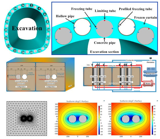
The Gongbei Tunnel, depicted in Figure 1, is a key project of the Zhuhai link of the Hong Kong–Zhuhai–Macao Bridge. It is located under the Gongbei Port and was constructed by underground excavation, with an average buried depth of 4–5 meters, over a total distance of 255 m and an excavation area of 336.8 m2, which is a typical shallow tunnel with large section. The geological conditions of the tunnel site are very complex, and most of them are unevenly developed saturated weak soil layers with high compressibility, high permeability and low strength, which can easily lead to uneven foundation settlement. Due to the large curvature of the plane axis of the tunnel, the PRM cannot ensure the construction accuracy of pipe jacking, and it is difficult to realize the water-stop lock connection between steel pipes, which cannot guarantee the water-sealing effect of the pipe roof. Following research and demonstrations, a new method called the freeze-sealing pipe roof (FSPR) method, depicted in Figure 2, was proposed. The essential difference between the FSPR and the freeze-sealing tube shed method in the design concept is that the pipe roof is formed by the close arrangement of large-diameter pipes as the bearing structure, and the pipe spacing is far less than the pipe diameter. The freezing tube is set inside the pipe wall to freeze the soil between the pipes and form a watertight underground space. Therefore, it replaces the original water sealing structure with a frozen curtain.
In the Gongbei Tunnel Project, 36 pipes with a diameter of 1600 mm were alternated around the circumference of the tunnel excavation, depicted in Figure 2. The circular freezing tubes were installed in the odd-numbered pipe (concrete pipe), and the limiting tubes were arranged away from the excavation section, with the main task of controlling the development of the frozen curtain in time to reduce frost heaving. The even-numbered pipe (hollow pipe) is used as a maintenance channel to facilitate internal maintenance and frozen soil monitoring. The profiled freezing-tube (formed by 125 × 125 × 8 mm angle steel) is directly welded onto the inner wall of the hollow pipe, as shown in Figure 3 and Figure 4. Considering the safety of the water sealing structure and the influence of frost heaving, the design average thickness of the frozen soil curtain in the buried excavation section of the Gongbei Tunnel is 2–2.6 m. According to the freezing construction scheme, the actual freezing time is 180 days, of which the active freezing period is 90 days.
However, this is the first application of FSPR. During the freezing construction of the Gongbei Tunnel, we encountered some practical problems, which could not be estimated by the theory of this new method. In particular, the profiled freezing-tube was designed to be made of equilateral angle steel and welded onto the inner wall of the hollow pipe. In the actual construction, many of these welds are arc and overhand welds, which have strict requirements and difficult manufacturing details. Furthermore, due to the existence of pipe jacking curvature, the welding quality cannot be guaranteed, leading to the frequent occurrence of refrigerant leakage accidents, resulting in huge maintenance costs. The ventilation condition in the long pipeline is poor, and a large number of welding operations have caused air pollution, potential safety hazards, and workers’ health effects. We often observed that the effect of horizontal freezing cannot achieve the expected purpose, which means a longer freezing time than intended. These problems not only bring difficulties to the construction and affect the progress but also restrict the further promotion of FSPR.
In this study, an improved design for improving the profiled freezing-tube was proposed to solve the above problems. By using a scale model test to verify the feasibility of the improved design, and a numerical model was established. The distribution characteristics of the freezing temperature field under two different configurations were compared by analyzing the test data and numerical simulation results, and the improvement results were explored to contribute to the improvement and promotion of FSPR in the future.
2. Scaled Model Test and Process
2.1. Scaling Laws
The scaling law equation of the temperature field can be defined as follows [29,30,31,32,33]:
where F0, K0, L0, and θ are as defined in the following equations.
The variable F0 is the Fourier criterion and is given by:
where a is the thermal conductivity of the material (m2/s), τ is time (h), and r is the radial thickness of the frozen soil wall (m).
The variable K0 is the Kossovich criterion and is given as:
where Q is the latent heat released during the freezing of the unit mass of soil (J/g), t is the temperature (°C), and c is the specific heat (J/(g·°C)).
If the model material is the same as the prototype material, the thermal conductivity scaling law Ca = 1 and the specific heat scaling law Cc = 1. The latent heat scaling law CQ = 1 can be obtained by guaranteeing that the model soil moisture content is the same as the prototype. It can be deduced from Equation (2) and Equation (3):
where Cτ is the time scaling law, Ct is the temperature scaling law, and Cl is the geometric scaling law, which is Cl =10 for this model test. The test discussed in this paper focused on the distribution of the temperature field, providing a comparison of the optimum results of the FSPR process. Because the tests were conducted at a partial scale, the saturated sand used in the test was reformulated according to the nature of the undisturbed soil at the Gongbei Tunnel project site to ensure the scaling law of materials.
The variable L0 is dimensionless and given as:
where ξ is the radial thickness of the frozen soil wall and r0 is the plane polar radius.
The variable θ is dimensionless and given as:
where t0 is the initial temperature of the soil, ty is the saline water temperature, td is the soil freezing temperature, and t is the temperature of any point in the frozen soil.
The velocity of saltwater in the freezing tube can be described by:
where v’ is the velocity of saltwater in the freezing tube of the model, and v is the velocity of saltwater in the freezing tube of the prototype.
According to the geometric scaling law selected (Cl =10), the dimensions of the pipe and the freezing-tube were obtained as shown in Table 1.
In the Gongbei Tunnel project, an 80-mm diameter main freezing tube carrying the refrigeration equipment (the blue circle in the concrete-filled pipe in Figure 2) was equipped with a flowmeter. The test presented in this paper used low-temperature saltwater directly (similar to the Gongbei Tunnel Project) and the freezing tube was replicated by a steel tube with a diameter of 8 mm. The velocity parameters are shown in Table 2.
2.2. Design of Model and Improvement of Profiled Freezing-tube
Due to the complexity of the engineering prototype, to study the temperature field difference of the hollow pipe in different configurations, the adjacent concrete pipe and hollow pipe, as well as the surrounding saturated sand, were selected as the research objects after comprehensive consideration of the test conditions. To address the limitations of the profiled freezing-tube used in the actual tunnel and considering the principle of substitution dictating the need to provide the same cross-sectional area of the tube, double 8-mm diameter circular freezing-tubes were used in place of the profiled freezing-tube on both sides of the hollow pipe. The double circular freezing-tubes were then wrapped with cement mortar and thus fixed to the interior of the hollow pipe as Configuration 2, shown in Figure 5 and Figure 6b. Compared to Configuration 1, this improvement provides a more conventional construction and installation method, replaces a large number of complex welding operations, and avoids the leakage of low-temperature brine during freezing, making it more environmentally friendly.
The size of the model box used was 2400 × 1200 × 1500 mm (W × H × L), constructed of a 6-mm thick steel plate with foam insulation board placed on the inner surfaces of the steel plate. Configuration 1 represents the profiled freezing-tube in the hollow pipe similar to the prototype, Configuration 2 represents the double circular freezing-tubes in the hollow pipe, the schematic section of the model box and an end view of the model are shown in Figure 6 and Figure 7, respectively. The concrete pipe (filled with C30 fine aggregate concrete) and the hollow pipe were arranged in the center of the box section, and the box was filled with saturated sand.
The test was conducted at the Liu Zhuang Coal Mine Project Department of Anhui Province, where direct cooling was provided by the field freezing equipment. Referring to the freezing parameters of the actual project and the temperature scaling law Ct = 1, a low temperature circulating saltwater refrigeration system was adopted in the test, providing an average temperature of −25 °C. The saltwater in the limiting-tube was heated by a thermostat heater to an average temperature of 9 °C. Red copper was selected as the tube material, and each separate freezing-tube was equipped with a set of independent switches. The freezing system used is illustrated in Figure 8.
2.3. Design of Monitoring System
In the experimental configuration, consisting of the concrete pipe and the hollow pipe with the profiled freezing-tube (Configuration 1), the temperature measurement points were set along the shared centerline of the two pipes (m1–m6), the vertical axis of the hollow pipe (v1–v6), and the horizontal axis of the hollow pipe (h1–h4), to study the law of the temperature field around the pipes, especially the horizontal and vertical directions of the hollow pipe. The temperature measurement points were spaced at 50 mm intervals from the faces of the pipes, as shown in Figure 9a. Similarly, the layout of the temperature measurement points of Configuration 2 was as shown in Figure 9b.
The main monitoring system consisted of a TML TDS-602 data logger and dozens of thermocouple sensors for temperature measurement, as shown in Figure 10. The range of the sensor varies from −200 °C to +800 °C, the accuracy is ±0.1 °C. A CW-500 digital temperature measurement system was used to collect the second set of data to ensure measurement accuracy and reliability. The measurement points for the two temperature measuring systems were symmetrically arranged about the transverse centerline of the box, as shown in Figure 11, in the vertical and horizontal locations shown for each configuration. The test data in this paper are based on the TDS-602 data logger. During the early stages of freezing, data were collected every 0.5 h, and during the later period of the freezing process, data were collected every 1 h. According to the specific circumstances of the testing device, the system can automatically collect data and monitor at even shorter time intervals if necessary.
2.4. Test Process
The water content, dry density, freezing point, and thermal conductivity of the saturated sand were measured before the test, as shown in Table 3. The test date, the temperature of the environment, the temperature of the saltwater, and the initial temperature of the sand in the box were recorded before the freezing began, as shown in Table 4 and Figure 12.
According to the design data of freezing construction of Gongbei Tunnel, the average thickness range of frozen soil curtain is 2–2.6 m and considering the geometric scaling law Cl = 10, it is determined that when the temperature of the measurement points on the centerline and 50 mm away from the contour line including m2, m6, m2* and m6* which dropped below −0.5 °C in the model test. This means that the thickness of the frozen soil wall between the concrete pipe and the hollow pipe reaches 260 mm, which can meet the design requirements. Combined with the project duration and time scaling law, the total freezing time of the test was set as 42 h. The refrigeration machine was then activated and the refrigerant temperature was completely reduced to the design temperature (−25 °C). The temperature change of the entire test area was regularly monitored by the test system until the end of the test. To study the effect of the limiting-tube, after the first 21 h of freezing time, the thermostat heater was turned on and the hot saltwater was circulated at 9 °C in the limiting tube, as in Figure 8 and Figure 12b.
3. Test results and Discussion
3.1. Vertical and Horizontal Measurement Points
The temperature measurement points in the two configurations are measured over 42 h of freezing to create temperature–time curves. The horizontal dashed line in each figure is a −0.5 °C (freezing point) reference line and the vertical dashed line is the time at which the limiting-tubes opened (21 h).
As can be seen from Figure 13, the temperature–time curve of all measurement points along the centerline shows an overall trend of decline and stabilization in both configurations. In each configuration, the curves of symmetrical position points coincide, and the point at the contour line shows the lowest temperature. From the changing trend of the curve, the temperature at each point decreased significantly in the first few hours, and the curves of Configuration 2 decreased more significantly. At 12 h, the temperature of m1 and m5 in Configuration 1 dropped below the freezing point, indicating that 160 mm thick frozen soil was formed between pipes, but the time in Configuration 2 was 5 h, 7 hours earlier than the former. In Table 5, t21 and t42 are the 21 h temperature and the 42 h temperature, respectively; V1 and V2 are the average cooling rate for the period from 0 h to 21 h and the cooling rates for the period from 21 h to 42 h, respectively. At 14 h, the temperature of m2* and m6* in Configuration 2 had all dropped below the freezing point, indicating that a frozen wall with a thickness of at least 260 mm had been formed between the pipes, 7 hours earlier than that in Configuration 1, and the average time was shortened by 33%. the average temperature of m2* and m6* in Configuration 2 was 3.75 °C lower than that of m2 and m6 in structure 1, and the average cooling rate V1 increased by 26%. After freezing for 21 h, the hot saltwater circulation in the limiting-tube was opened and some of the temperature curves in both configurations rise significantly, most obviously for the closest point to the concrete pipe. The V2 of m2* and m6* are positive numbers, indicating that the temperature of these points underwent a certain recovery from their lowest temperature, but remained below the freezing point, which proves that the limiting-tube has a partial limiting effect on the continuous temperature reduction, especially in the area with lower temperature. After 24 h, the temperature curve for each measuring point is close to a horizontal line, indicating that the temperature change is very small and the development of the temperature field has been gradually stabilized. At 42 h, the average temperature of m2* and m6* in Configuration 2 was 1.9 °C lower than that of m2 and m6 in Configuration 1. Although both configurations ultimately meet the requirements of the test design, it is clear that the improved results are superior and reflect the shorter time and lower temperature. Other points along the centerline also support these conclusions.
It can be seen from Figure 14, that the stabilization and leveling of the curves for the vertical measurement points along the hollow pipe are similar to the centerline points in Figure 13. From the comparison of curve changes, it can be seen that the temperature in Configuration 2 still drops faster. Table 6 compares the temperature–time curves and data of the vertical points 50 mm away from the hollow pipe wall in the two configurations. During the first 21 h of the test, v2* and v6* in Configuration 2 showed a higher average cooling rate V1, and the temperature of both points dropped below the freezing point at 16h, while v2 and v6 in Configuration 1 did not reach the same result until 33 h, with an average time reduction of 46%. After 21 h, no obvious rebound of any curve was found, so it can be inferred that the influence of the limiting-tube more significant in the near range than in the far range. It can also be seen from the data of V2 in Table 6 that in the last 21 h of the test, the average cooling rate of v2* and v6* was lower, indicating that the freezing temperature field above the hollow pipe wall in Configuration 2 entered a stable state earlier than that in Configuration 1, so it can be concluded that the freezing effect of Configuration 2 is also more excellent in the vertical position of the hollow pipe, and the data of other measurement points have also supported these conclusions.
As can be seen from Table 7, h2* and h3* in Configuration 2 have lower temperatures and higher average cooling rate V1. At 10 h, the temperature of h2* in Configuration 2 has dropped below the freezing point, which is 9 h earlier than that of h2 in Configuration 1, 47% shorter. At 21 h, the temperature of h2* and h3* in Configuration 2 is 3 °C and 3.4 °C lower than that of h2 and h3 in Configuration 1, respectively. At the end of the test, the temperature of h3* is −2.2 °C, while the temperature of h3 has not fallen below the freezing point. It can be concluded that the improved freezing tube can also provide a better horizontal freezing effect.
3.2. Circumferential Points around The Hollow Pipe
The temperature–time curves of points around the hollow pipe in Configurations 1 and 2 are compared in Figure 15 and Figure 16, respectively, at circumferential distances of 0 mm and 50 mm. It can be seen in these figures that the temperature of the measuring points on the right side is consistently lower than that of the vertical owing to the location of the freezing tubes near the right side of the hollow pipe; thus, the cooling rate is higher as well. The temperature curves of each measuring point at a circumferential distance of 50 mm are all very close, and their cooling rates are the same. As these measurement points are farther away from the pipe wall, the temperature curve in each direction tends to grade level and the temperature difference overtime is no longer obvious. An in-depth analysis determined that the freezing tube on the inside of the hollow pipe first cools the pipe wall, and then reduces the temperature of the surrounding soil via the surface area of the pipe.
4. Numerical Simulation and Discussion
4.1. Model Establishment and Verification of Test Results
In order to study in a more comprehensive way of the distribution of freezing temperature field and the difference of frozen soil wall thickness in different positions under the two configurations, the corresponding numerical models were established. Take Configuration 2 as an example, the (Finite Element Modeling) FEM software COMSOL MULTIPHYSICS (COMSOL Multiphysics® v. 5.4. COMSOL AB, Stockholm, Sweden. 2018) was used to simulate the two-dimensional temperature field of the test models, as in Figure 17. The area was a square with a length of 1.2 m, consisting of soil and two steel pipes (the size was the same as the test model). Because the heat transfer in porous media module can effectively simulate the heat transfer phenomenon in soil, it was adopted as the calculation module [34,35,36]. The grid system of the computational domain is created using unstructured triangle element, and its density is higher near the steel pipes and the freezing tubes, as in Figure 18. The numerical model used in this paper has a minimum element size of 0.42 mm, an average element quality of 0.8261 and a minimum element quality of 0.04037, which means that the mesh element quality is good and the calculation results can converge [37].
As shown in the Figure 17, this model has three boundaries: the first boundary is the soil boundary, which is counted as insulation, and the initial value of the soil temperature is set to 20 °C. The second boundary and the third boundary are the freezing-tube wall and limiting-tube wall respectively, which are considered to constitute the Dirichlet boundary condition with temperatures set at −25 °C and 9 °C, respectively. The thermophysical properties of soil, concrete, steel pipe, cement, and air are based on laboratory tests, as shown in Table 8.
The temperature–time curves of the simulated measurement points m2 and m2* are compared with the test data in Figure 19. The numerical simulation results are in good agreement with the test results, which indicates the numerical simulation results are accurate. Therefore, more comprehensive can be conducted.
4.2. Freezing Temperature Field Simulation Results Discussion
Figure 20 and Figure 21 compares the distribution of freezing temperature field at 21 h and the average thickness of frozen soil wall at different positions in the two configurations. It can be seen that in both configurations, the frozen soil wall around the concrete pipe develops faster than the hollow pipe, and a certain amount of thickness has been formed between the two pipes, indicating that the water sealing structure between the pipes has initially formed. Because of the position of the freezing tube, the temperature in the horizontal direction is lower, the shape of the isotherm is approximately elliptical in the far range. The significant differences in the thickness of the frozen soil wall under the two configurations were mainly on the right side of the hollow pipe, the vertical direction of the hollow pipe and between the two pipes, which increased by 34%, 20%, and 12% respectively in Configuration 2.
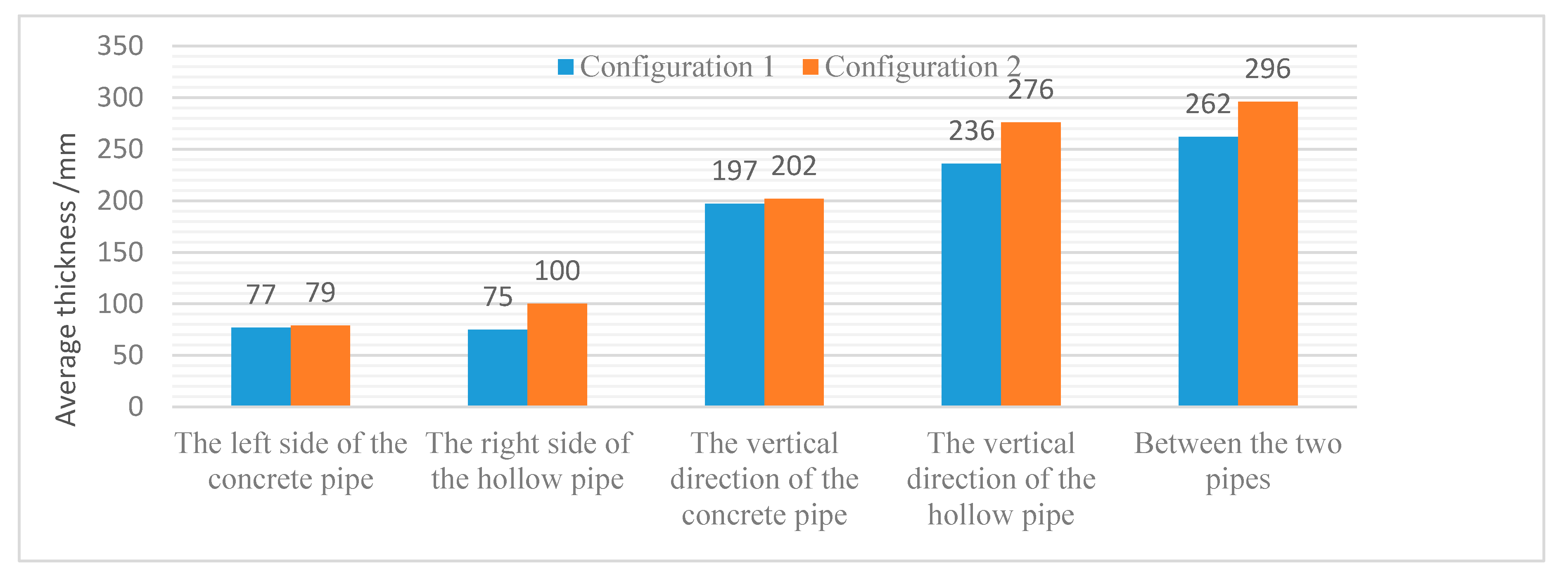
From Figure 22 and Figure 23, it can be seen that after 42 h, the continuous action of the limiting-tube has a certain influence on the temperature field around the concrete pipe, especially the temperature in the range close to the limiting-tube has increased significantly. The average thickness of the frozen soil wall in the vertical direction of the concrete pipe in the two configurations decreased by 46 mm and 58 mm compared with that at 21 h and was also significantly lower than that of the hollow pipe in the vertical direction at 42 h, which indicates that the limiting-tube can limit the excessive development of the frozen soil wall within a certain range, to avoid the adverse impact of frost heave on the ground building structure. The size of the frozen soil wall around the hollow tube has exceeded that of the concrete tube, compared with the first 21 h of freezing, the development of the last 21 h is slower, indicating that the temperature field in the model has entered a relatively stable-stage. As the focus of the research, the thickness of the frozen soil wall between the two pipes still keeps a small increase and can meet the design requirements. Configuration 2 can still show better freezing performance, compared with Configuration 1, the average thickness of frozen soil wall on the right side of the hollow pipe, the vertical direction of the hollow pipe and between the two pipes increased by 33%, 17%, and 13%, respectively, which means that better results can be achieved in the same freezing time.
5. Conclusions
(1) To solve the practical problems existing in the construction of the Gongbei Tunnel, an improved design was proposed for the profiled freezing-tube in FSPR. Using scaled model tests and numerical simulation, the difference of temperature field distribution and the variation in the freezing performance were studied.
(2) In the scale model test, it is very convenient to make and install the double circular freezing-tubes in Configuration 2, which can be expected to replace a large number of profiled freezing-tube manufacturing and welding operations in actual project construction, solve practical problems such as welding difficulties, refrigerant leakage, air pollution, and significantly improve the quality of engineering.
(3) Through the comparative analysis of experimental data and numerical calculation results, it can be concluded that: in the early stage of the freezing process, the temperature of the surrounding soil drops very rapidly, the temperature–time curve of all measurement points shows an overall trend of decline and stabilization in both configurations. With the passage of freezing time, the rate of temperature decline gradually decreases and the temperature curve tends to level off. At 21 h, the range of frozen soil wall around the concrete pipe is larger than that around the hollow pipe, and the average thickness between the pipes is 252 mm and 281 mm respectively, indicating that the water sealing structure has been formed. In Configuration 2, the average temperature of the point 50 mm away from the contour line of the centerline between two pipes and the vertical line of the hollow pipe is 3.75 °C and 4.65 °C lower than that of Configuration 1, respectively. The average temperature cooling rate V1 increases by 26% and 34%, and the freezing time required for the temperature to drop below the freezing point is 33% and 46% shorter, respectively. The development principle of freezing temperature field is that the freezing tube on the inside of the pipe first cools the pipe wall, and then reduces the temperature of the surrounding soil via the surface area of the pipe. The opening of the limiting-tube makes the temperature of the nearby measurement points rise significantly in the period from 21 h to 24 h. After 24 h, the temperature of these points hardly changes and the temperature curve tends to level. By the end of the test, under the influence of the freezing tube and the limiting-tube, the temperature field was gradually stabilized, and the range of the frozen soil wall around the hollow pipe finally exceeded that of the concrete pipe, indicating that the limiting-tube could limit the excessive development of the frozen soil wall within a certain range, to avoid the adverse impact of frost heave on the ground building structure. The significant difference in the temperature field between the two configurations is reflected in the horizontal direction of the hollow pipe, the vertical direction of the hollow pipe, and between the two pipes. The average thickness of the frozen soil wall at these locations increased by 33%, 17%, and 13% in Configuration 2, respectively. In general, the proposed optimization scheme can make the surrounding soil more quickly frozen and provide an enhanced freezing effect under the same conditions, which means that it can significantly shorten the construction period of underground excavation and reduce the cost of maintenance, which is worth promoting in similar projects in the future.
Author Contributions
H.C. (Hua Cheng) and Z.W. proposed the idea of this research work and conceived the tests; Z.Y., H.C. (Haibing Cai) and Y.D. performed the tests; Y.D. and C.R. wrote the paper. All authors have read and agreed to the published version of the manuscript.
Funding
This research was funded by National Natural Science Foundation of China [grant numbers 51878005, 51778004, 51374010].
Conflicts of Interest
The authors declare no conflict of interest.
Data Availability
The data used to support the findings of this study are available from the corresponding author upon request.
References
- Cheng, H. Theory and Technology of Shaft Sinking by Freezing Method for Deep Alluvium, 1st ed.; Science Press: Beijing, China, 2016; pp. 118–120. (In Chinese) [Google Scholar]
- Cheng, H.; Yao, Z.S.; Zhang, J.S. A model test study on the effect of freeze heaving and thaw subsidence for tunnel construction with artificial horizontal ground freezing. China Civ. Eng. J. 2007, 40, 80–85. [Google Scholar] [CrossRef]
- Ma, W. Review and prospect of the studies of ground freezing technology in China. J. Glaciol. Geocryol. 2001, 23, 218–224. [Google Scholar] [CrossRef]
- Li, S.; Lai, Y.; Zhang, M.; Zhang, S. Minimum ground pre-freezing time before excavation of Guangzhou subway tunnel. Cold Reg. Sci. Technol. 2006, 46, 181–191. [Google Scholar] [CrossRef]
- Yang, Y.; Lai, Y.; Chang, X. Laboratory and theoretical investigations on the deformation and strength behaviors of artificial frozen soil. Cold Reg. Sci. Technol. 2010, 64, 39–45. [Google Scholar] [CrossRef]
- Cai, H.; Li, S.; Liang, Y.; Yao, Z.; Cheng, H. Model test and numerical simulation of frost heave during twin-tunnel construction using artificial ground-freezing technique. Comput. Geotech. 2019, 115, 103155. [Google Scholar] [CrossRef]
- Yao., Z.S.; Cai, H.B.; Cheng, H. The Model Test Study on Frost Heaving and Melting Sedimentation of Subway Tunnel Construction with Manual Level Freezing Method. Advanced Materials Research. 2011, 243, 3476–3483. [Google Scholar] [CrossRef]
- Afshani, A.; Akagi, H. Artificial ground freezing application in shield tunneling. Jpn. Geotech. Soc. Spéc. Publ. 2015, 3, 71–75. [Google Scholar] [CrossRef] [Green Version]
- Yan, Q.; Xu, Y.; Yang, W.-B.; Geng, P. Nonlinear Transient Analysis of Temperature Fields in an AGF Project used for a Cross-Passage Tunnel in the Suzhou Metro. KSCE J. Civ. Eng. 2018, 22, 1473–1483. [Google Scholar] [CrossRef]
- Ji, Y.; Zhou, G.; Zhou, Y.; Hall, M.R.; Zhao, X.; Mo, P.-Q. A separate-ice based solution for frost heaving-induced pressure during coupled thermal-hydro-mechanical processes in freezing soils. Cold Reg. Sci. Technol. 2018, 147, 22–33. [Google Scholar] [CrossRef]
- Lai, Y.; Zhang, S.; Yu, W. A new structure to control frost boiling and frost heave of embankments in cold regions. Cold Reg. Sci. Technol. 2012, 79, 53–66. [Google Scholar] [CrossRef]
- Zhou, J.; Tang, Y. Artificial ground freezing of fully saturated mucky clay: Thawing problem by centrifuge modeling. Cold Reg. Sci. Technol. 2015, 117, 1–11. [Google Scholar] [CrossRef]
- Zhu, H.H.; Yan, Z.G.; Li, X.Y.; Liu, X.Z.; Shen, G.P. Analysis of Construction Risks for Pipe-roofing Tunnel in Saturated Soft Soil. Chin. J. Rock Mech. Eng. 2005, 24, 5549–5554. [Google Scholar]
- Wang, X.; Dong, P.; Chen, S. Preparation of Macroporous Al2O3 by Template Method. Acta Physico Chimica Sin. 2006, 22, 831–835. [Google Scholar] [CrossRef]
- Brun, B.; Ha, H. Underground Line U5 ‘Unter Den Linden’ Berlin, Germany Structural and Thermal Fe-Calculations for Ground Freezing Design. In Proceedings of the International Conference on Numerical Simulation of Construction Processes in Geotechnical Engineering for Urban Environment, Bochum, Germany, 23–24 March 2006; pp. 225–232. [Google Scholar]
- Kamakura, T.; Aso, T.; Hamaguchi, K.; Inoue, H. Development of tunnel expansion method (SR-J) for underground highway junction. In Proceedings of the 60 Annual Conference of the Japan Society of Civil Engineers, Tokyo, Japan, 7–9 September 2005; Volume 6, pp. 165–166. [Google Scholar]
- Hamaguchi, K.; Yabe, Y.; Yoshitake, K. Development of small diameter shield combined large-section widening method (SR-JP). In Proceedings of the 61 Annual Conference of the Japan Society of Civil Engineers, Kusatsu, Japan, 20 September 2006; Volume 61, pp. 139–140. [Google Scholar]
- Ueda, Y.; Ohrai, T.; Yamamoto, M. Improvement of Bending Strength of Frozen Soil Beam Reinforced by Steel Pipe. Doboku Gakkai Ronbunshu 2001, 12, 81–90. [Google Scholar] [CrossRef] [Green Version]
- Pimentel, E.; Papakonstantinou, S.; Anagnostou, G. Numerical interpretation of temperature distributions from three ground freezing applications in urban tunnelling. Tunn. Undergr. Space Technol. 2012, 28, 57–69. [Google Scholar] [CrossRef]
- Pimentel, E.; Sres, A.; Anagnostou, G. Large-scale laboratory tests on artificial ground freezing under seepage-flow conditions. Géotechnique 2012, 62, 227–241. [Google Scholar] [CrossRef]
- Zhang, P.; Ma, B.; Zeng, C.; Xie, H.; Li, X.; Wang, D. Key techniques for the largest curved pipe jacking roof to date: A case study of Gongbei tunnel. Tunn. Undergr. Space Technol. 2016, 59, 134–145. [Google Scholar] [CrossRef]
- Hu, X.; She, S. Study of Freezing Scheme in Freeze-Sealing Pipe Roof Method Based on Numerical Simulation of Temperature Field. ICPTT 2013 2012, 1798–1805. [Google Scholar] [CrossRef]
- Hu, X.D.; Ren, H.; Chen, J.; Cheng, Y.; Zhang, J. Model test study of the active freezing scheme for the combined pipe-roof and freezing method. Mod. Tunn. Technol. 2014, 51, 92–98. [Google Scholar] [CrossRef]
- Hu, X.; Fang, T. Numerical Simulation of Temperature Field at the Active Freeze Period in Tunnel Construction Using Freeze-Sealing Pipe Roof Method. Soil Behav. Geomechanics 2014. [Google Scholar] [CrossRef]
- Hu, X.D.; Fang, T.; Guo, X.D.; Ren, H. Temperature field research on thawing process of Freeze-Sealing Pipe Roof Method in Gong-bei Tunnel by in-situ prototype test. J. China Coal Soc. 2017, 42, 1700–1705. [Google Scholar] [CrossRef]
- Ren, H.; Hu, X.D.; Chen, J.; Zhang, J. Study on Freezing Effect and Operation of Profiled Enhancing Freezing-tube in Freeze-sealing Pipe Roof. Tunn. Constr. 2015, 35, 1169–1175. [Google Scholar] [CrossRef]
- Kaasik, K.; Lee, C.C. Reciprocal regulation of haem biosynthesis and the circadian clock in mammals. Nature 2004, 430, 467–471. [Google Scholar] [CrossRef] [PubMed]
- Hu, J.; Hong, W.; Zeng, H.; Liu, Y.; Li, Y.P. Numerical analysis of temperature field of new pipe-roof freezing method. J. Railw. Sci. Eng. 2016, 13, 1165–1172. [Google Scholar] [CrossRef]
- Sun, J.-Y.; Tong, J. Fracture toughness properties of three different biomaterials measured by nanoindentation. J. Bionic Eng. 2007, 4, 11–17. [Google Scholar] [CrossRef]
- Cui, G.X.; Lu, Q.G. Study on law of thickness and deformation of ice-wall by using models. J. China Coal Soc. 1992, 17, 37–47. [Google Scholar] [CrossRef]
- Cui, G.X. The principle of model test for freezing shaft sinking. J. China Univ. Mining Technol. 1989, 18, 59–68. [Google Scholar]
- Zhang, Z.; Boyland, A.J.; Sahu, J.K.; Clarkson, W.A.; Ibsen, M. Single frequency Tm-doped fibre DBR laser at 1943 nm. In Proceedings of the CLEO/Europe—EQEC 2009—European Conference on Lasers and Electro-Optics and the European Quantum Electronics Conference, Munich, Germany, 14–19 June 2009; Volume 28, p. 1. [Google Scholar] [CrossRef] [Green Version]
- Taylor, R.N. Geotechnical Centrifuge Technology, 1st ed.; Blackie Academic & Professional: London, UK, 1994; pp. 273–280. [Google Scholar]
- Cai, H.B.; Cheng, H.; Yao, Z.S.; Wang, H. Numerical analysis of ground displacement due to orthotropic frost heave of frozen soil in freezing period of tunnel. Chin. J. Rock Mechan. Eng. 2015, 34, 1667–1676. [Google Scholar] [CrossRef]
- Yuanming, L.; Songyu, L.; Ziwang, W.; Wenbing, Y. Approximate analytical solution for temperature fields in cold regions circular tunnels. Cold Reg. Sci. Technol. 2002, 34, 43–49. [Google Scholar] [CrossRef]
- Hu, X.-D.; Fang, T.; Han, Y.-G. Mathematical solution of steady-state temperature field of circular frozen wall by single-circle-piped freezing. Cold Reg. Sci. Technol. 2018, 148, 96–103. [Google Scholar] [CrossRef]
- COMSOL Multiphysics Reference Manual. 2018. Available online: https://doc.comsol.com/5.4/doc/com.comsol.help.comsol/COMSOL_ReferenceManual.pdf (accessed on 15 August 2020).
Figure 1.
Geographic Map of Gongbei Tunnel.
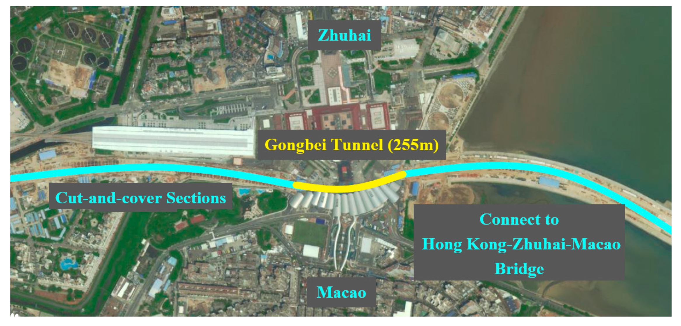
Figure 2.
Schematic Diagram of Freeze-Sealing Pipe Roof (FSPR).

Figure 3.
Schematic Diagram of Hollow pipe and Profiled Freezing-Tube.
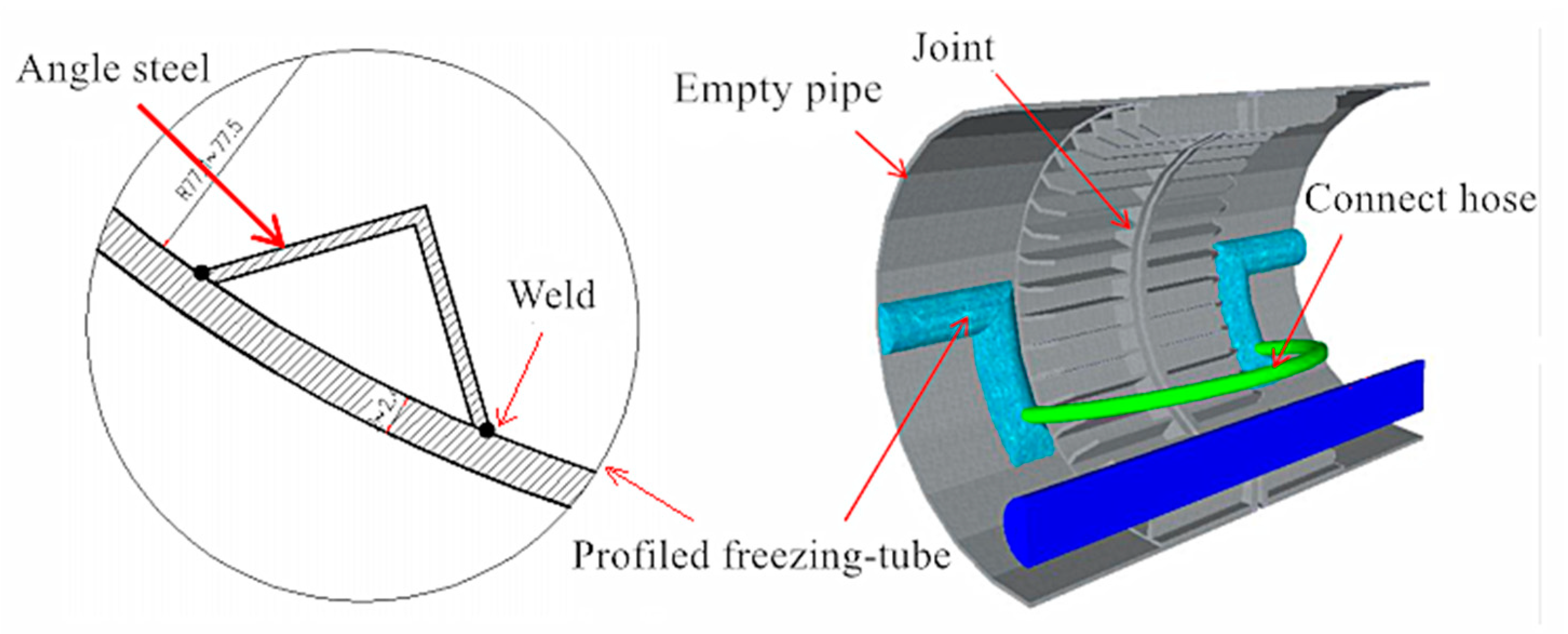
Figure 4.
Interior of Hollow Pipe showing Profiled Freezing-Tube.
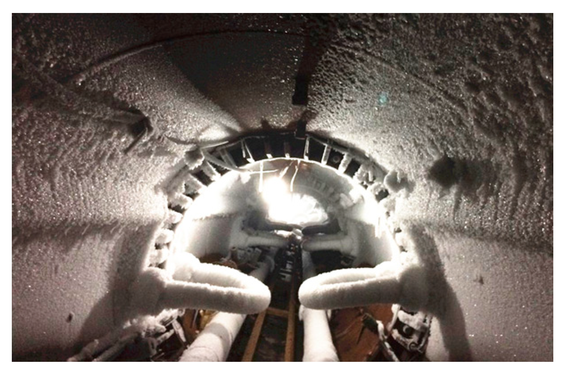
Figure 5.
Improved Design for Profiled Freezing-Tube.
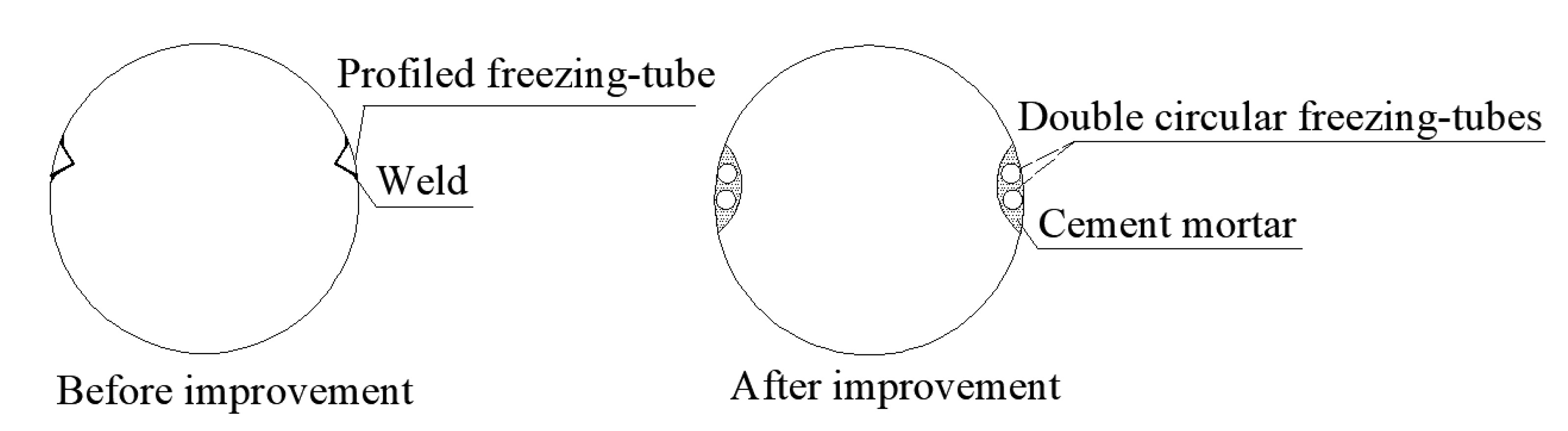
Figure 6.
Exterior view of model. (a) Model showing profiled freezing-tube (Configuration 1). (b) Model showing double circular freezing-tubes (Configuration 2).
Figure 6.
Exterior view of model. (a) Model showing profiled freezing-tube (Configuration 1). (b) Model showing double circular freezing-tubes (Configuration 2).

Figure 7.
Schematic Diagram of Model Box Section (mm).
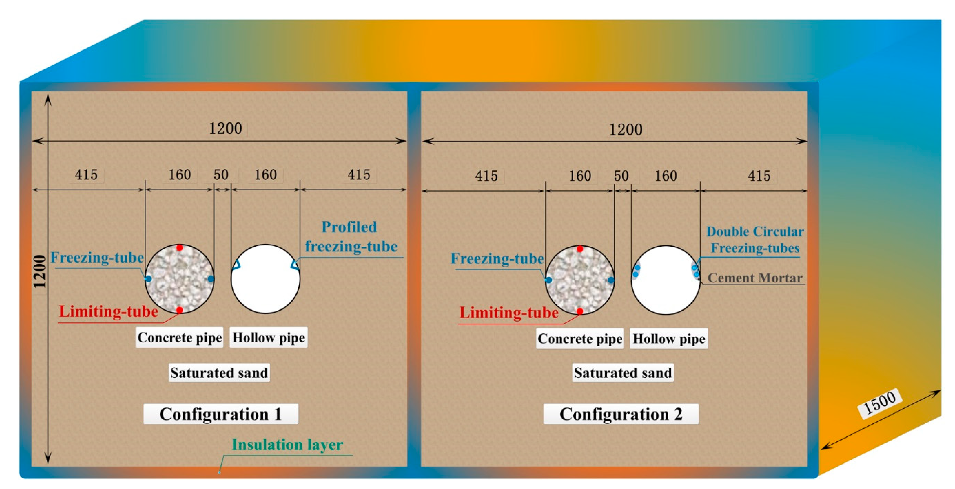
Figure 8.
Plane Diagram of the Freezing System.

Figure 9.
Layout of Temperature Measurement Points (mm): (a) Configuration 1, (b) Configuration 2.

Figure 10.
TDS-602 Data Logger.
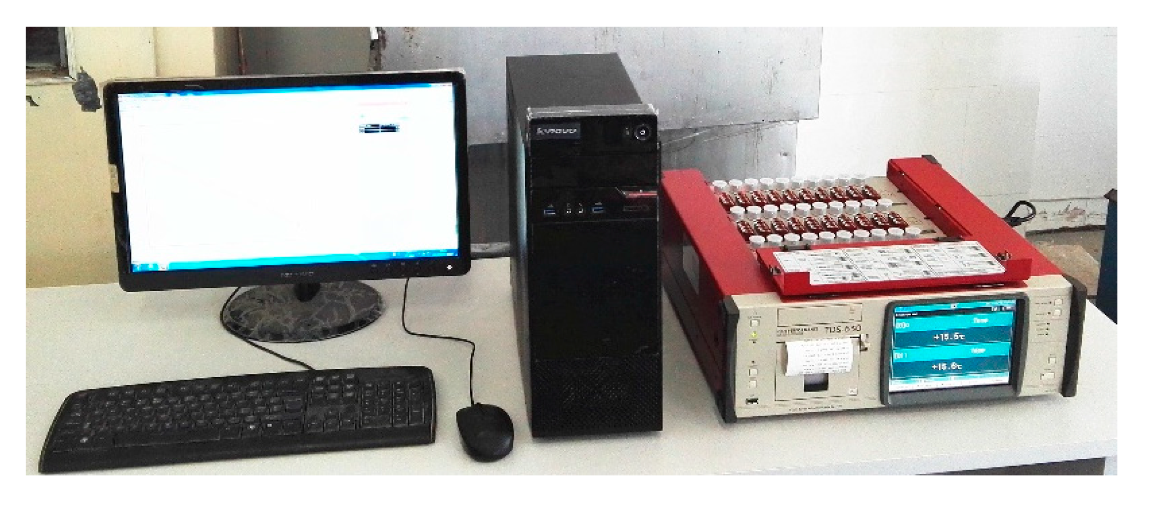
Figure 11.
Monitoring Location of Two Systems.

Figure 12.
Temperature–time curves of saltwater in freezing-tube and limiting-tube: (a) low-temperature saltwater in freezing-tube; (b) hot saltwater in limiting-tube.
Figure 12.
Temperature–time curves of saltwater in freezing-tube and limiting-tube: (a) low-temperature saltwater in freezing-tube; (b) hot saltwater in limiting-tube.
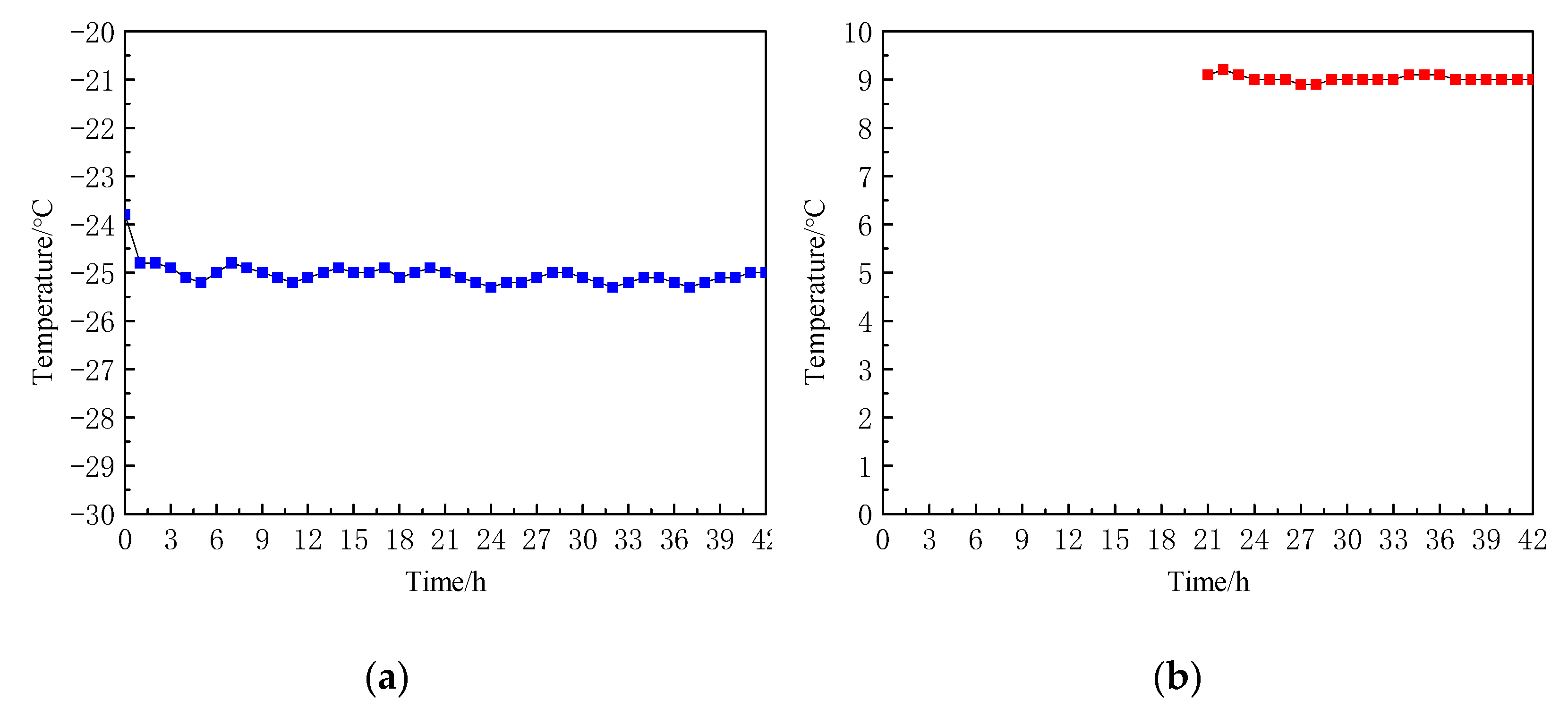
Figure 13.
Temperature–time curves of centerline points: (a) Configuration 1; (b) Configuration 2.
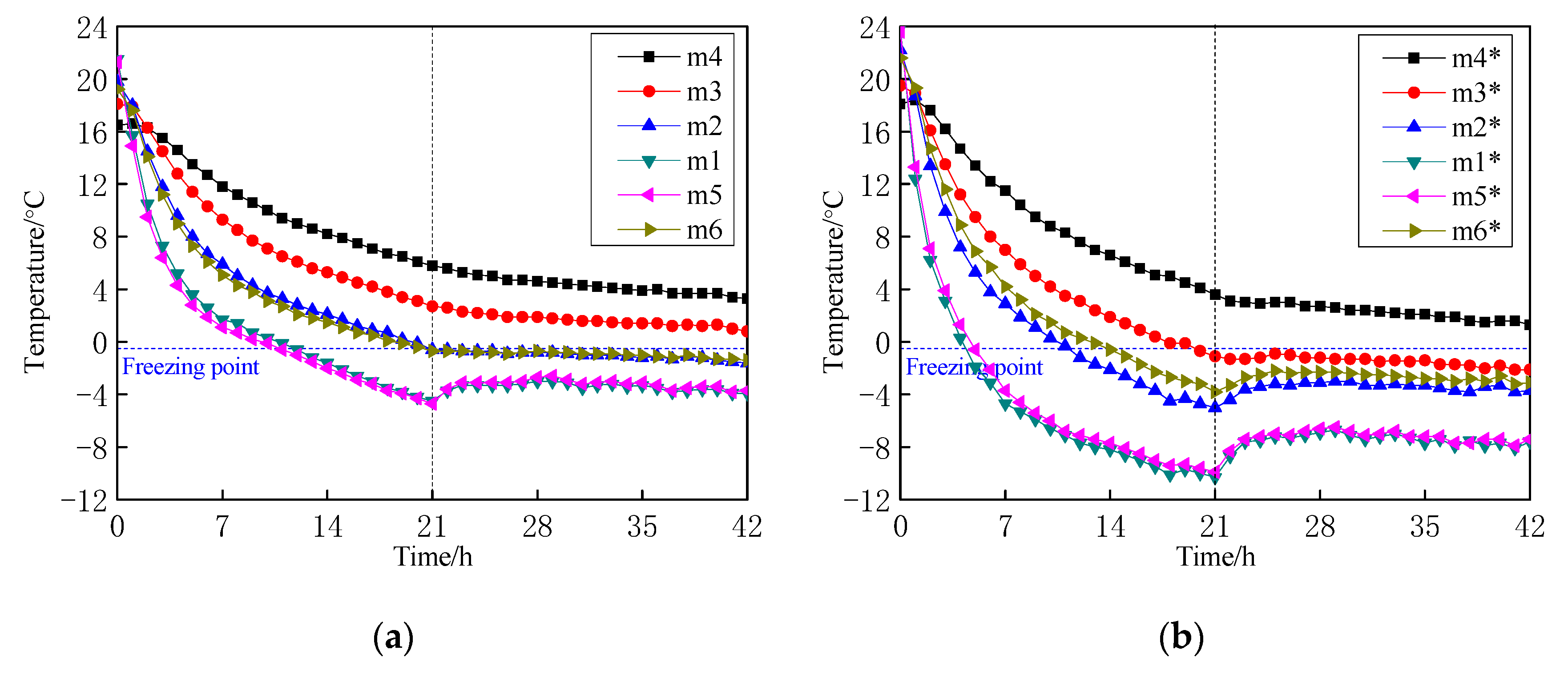
Figure 14.
Temperature-Time Curves of Vertical Points of Hollow pipe: (a) Configuration 1; (b) Configuration 2.
Figure 14.
Temperature-Time Curves of Vertical Points of Hollow pipe: (a) Configuration 1; (b) Configuration 2.
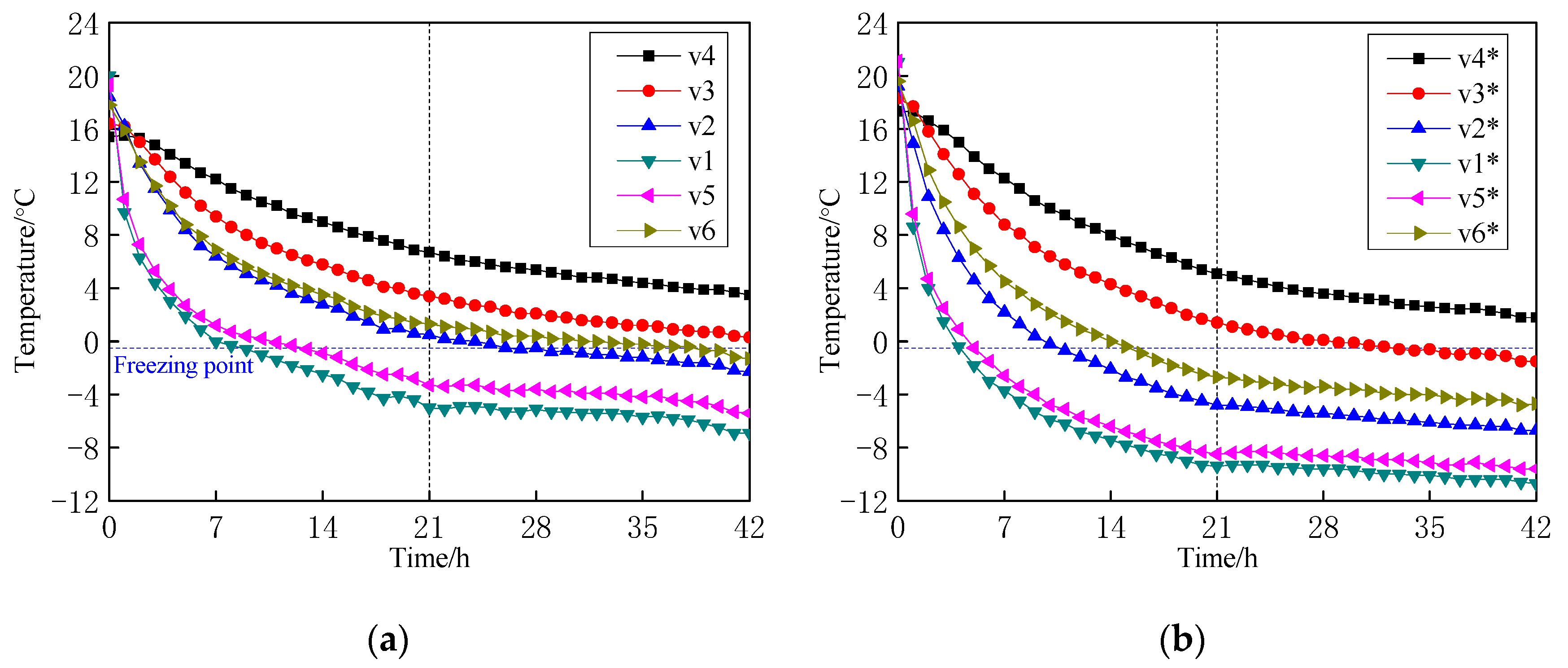
Figure 15.
Temperature–time curves of circumferential points of Configuration 1: (a) circumferential 0 mm; (b) circumferential 50 mm.
Figure 15.
Temperature–time curves of circumferential points of Configuration 1: (a) circumferential 0 mm; (b) circumferential 50 mm.
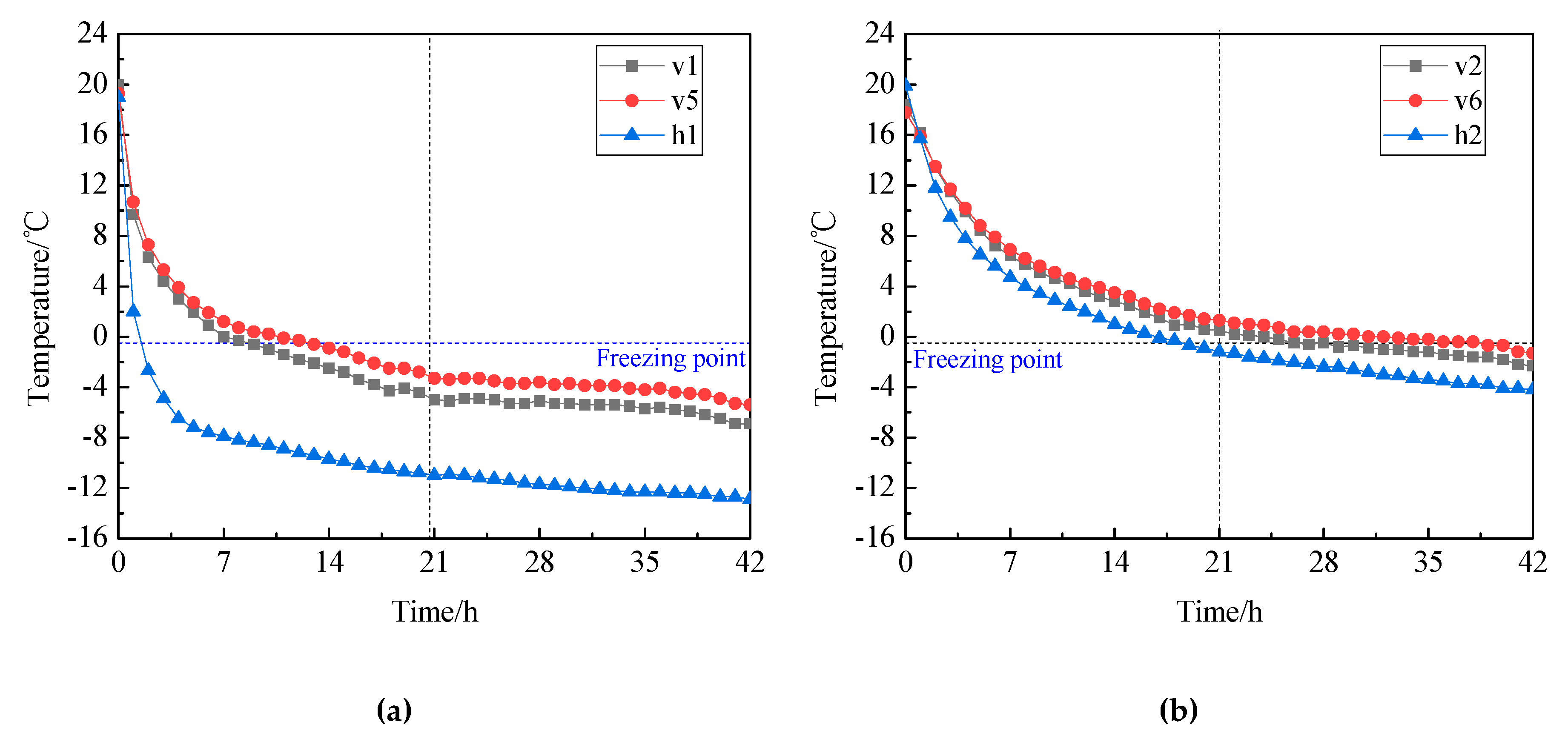
Figure 16.
Temperature–time curves of circumferential points of Configuration 2: (a) circumferential 0 mm; (b) circumferential 50mm.
Figure 16.
Temperature–time curves of circumferential points of Configuration 2: (a) circumferential 0 mm; (b) circumferential 50mm.
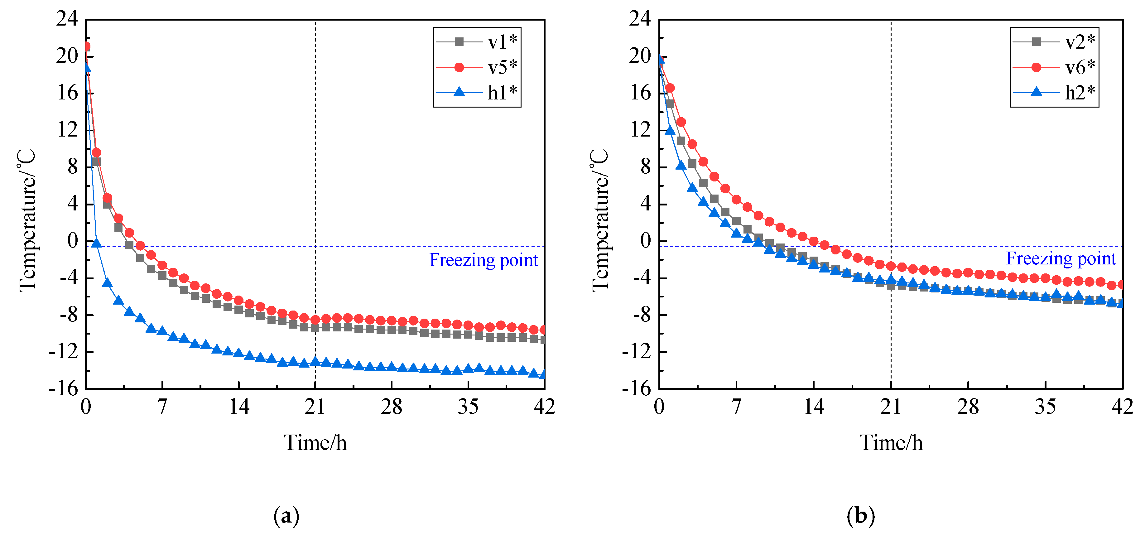
Figure 17.
Illustration of Numerical Model (Configuration 2).
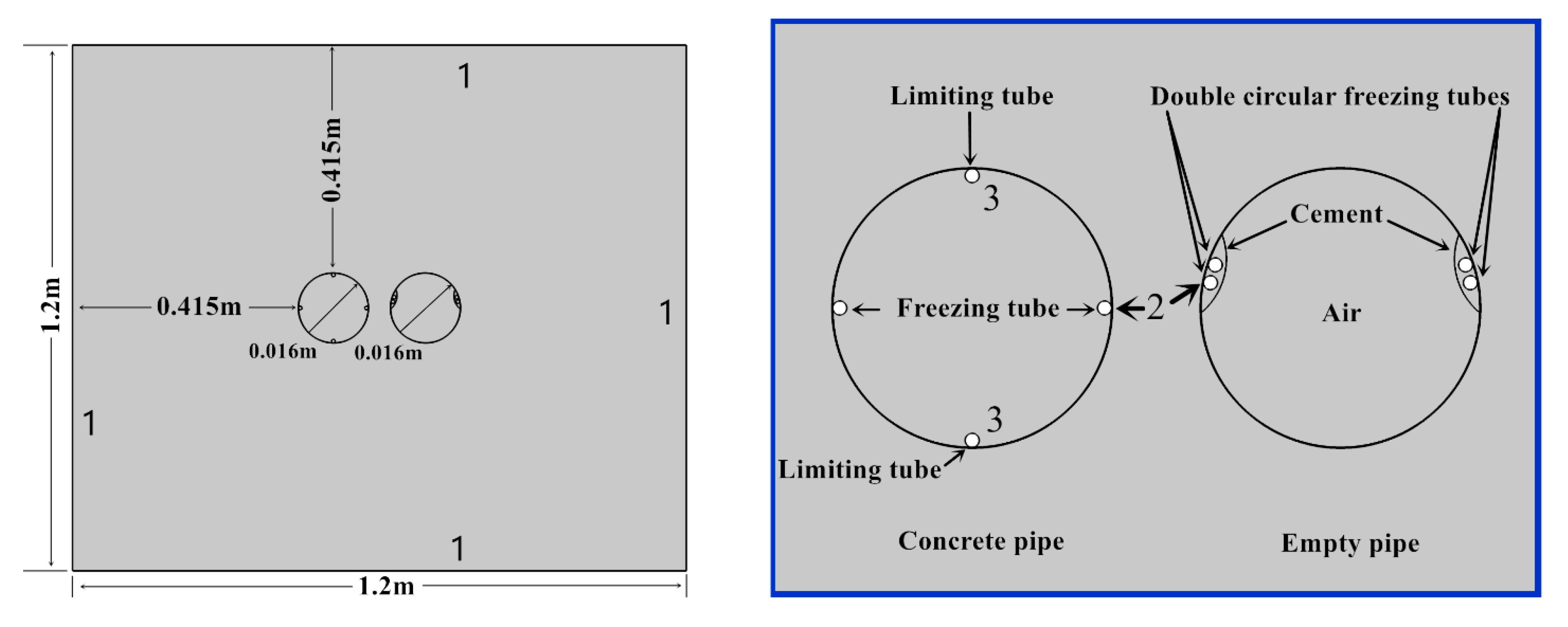
Figure 18.
Schematic Diagram of Grid System of Numerical Model (Configuration 2).
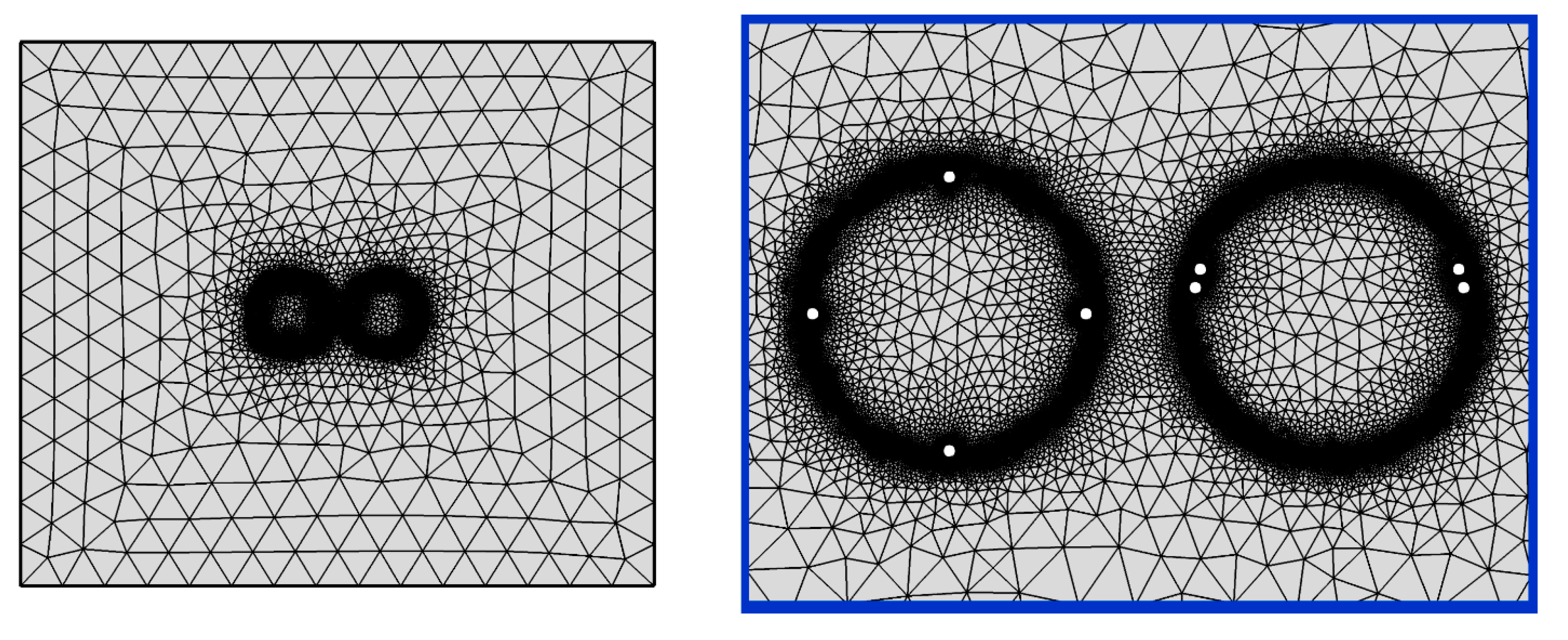
Figure 19.
Comparison of simulated data and experimental data: (a) m2 (Configuration 1), (b) m2* (Configuration 2).
Figure 19.
Comparison of simulated data and experimental data: (a) m2 (Configuration 1), (b) m2* (Configuration 2).
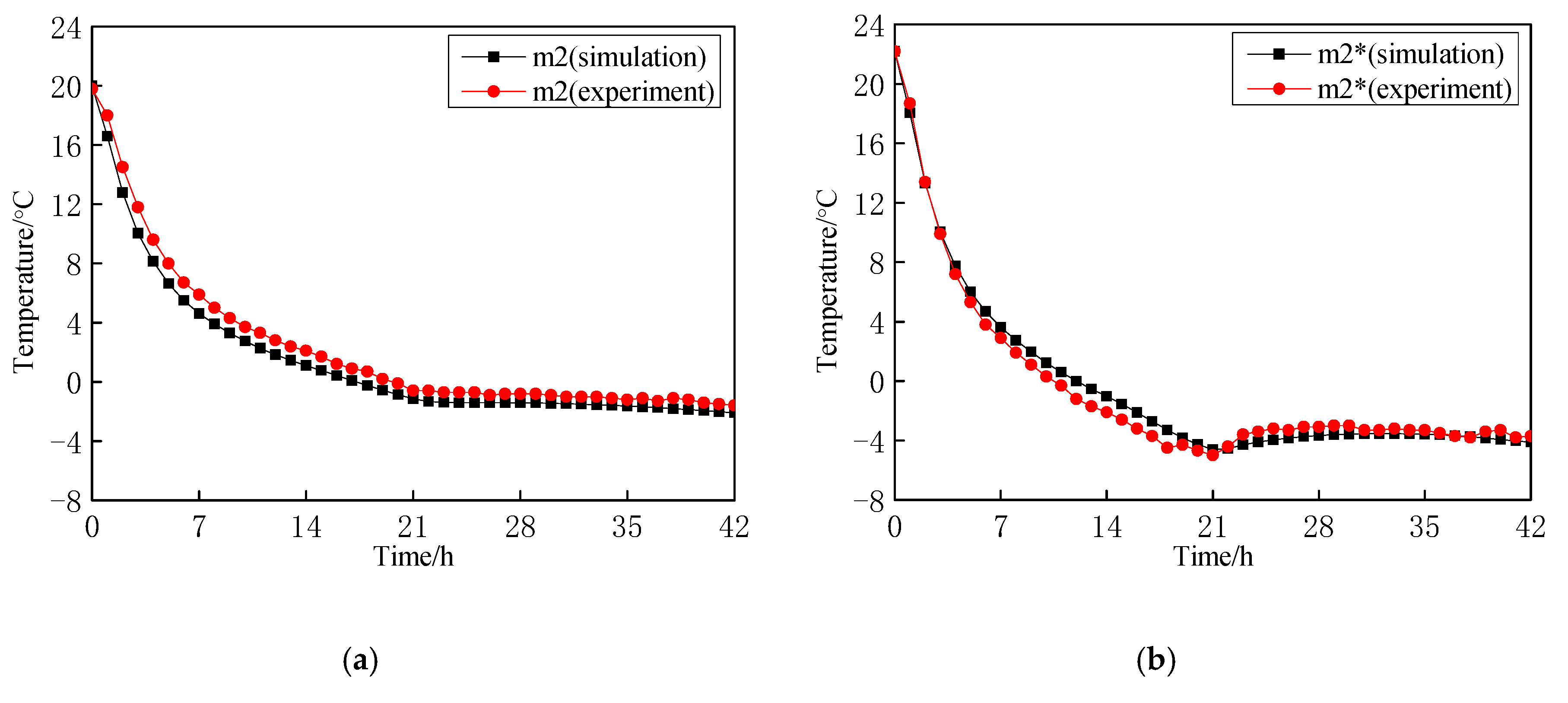
Figure 20.
Freezing temperature field at 21 h: (a) Configuration 1, (b) Configuration 2.
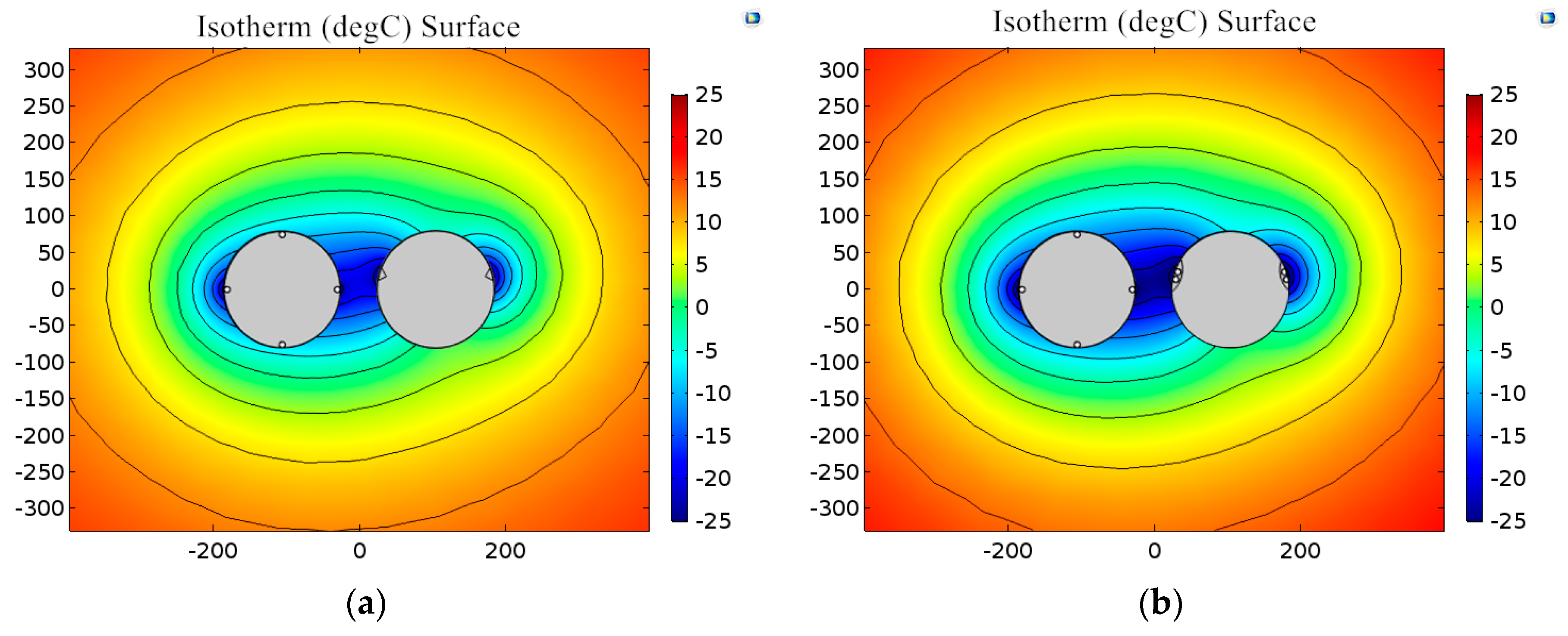
Figure 21.
Average thickness of frozen soil wall in different positions at 21 h.
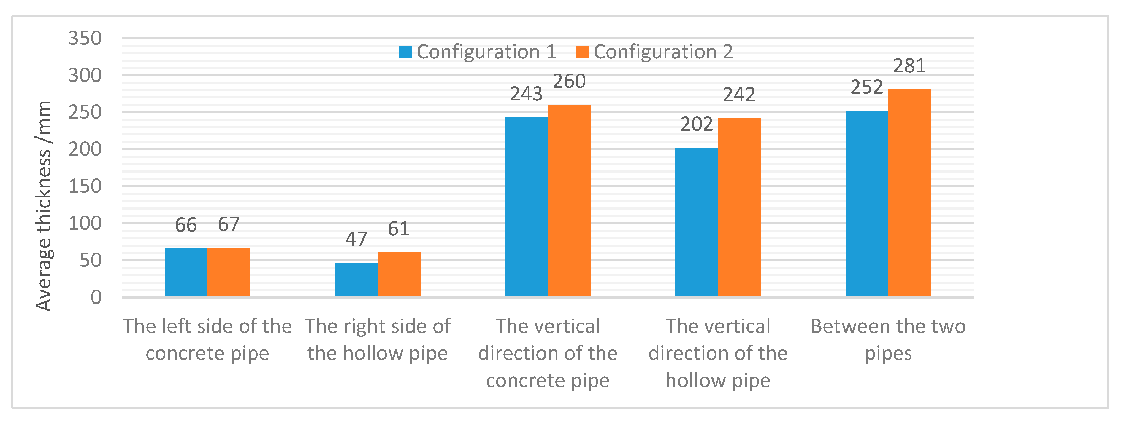
Figure 22.
Freezing temperature field after 42 hours: (a) Configuration 1, (b) Configuration 2.
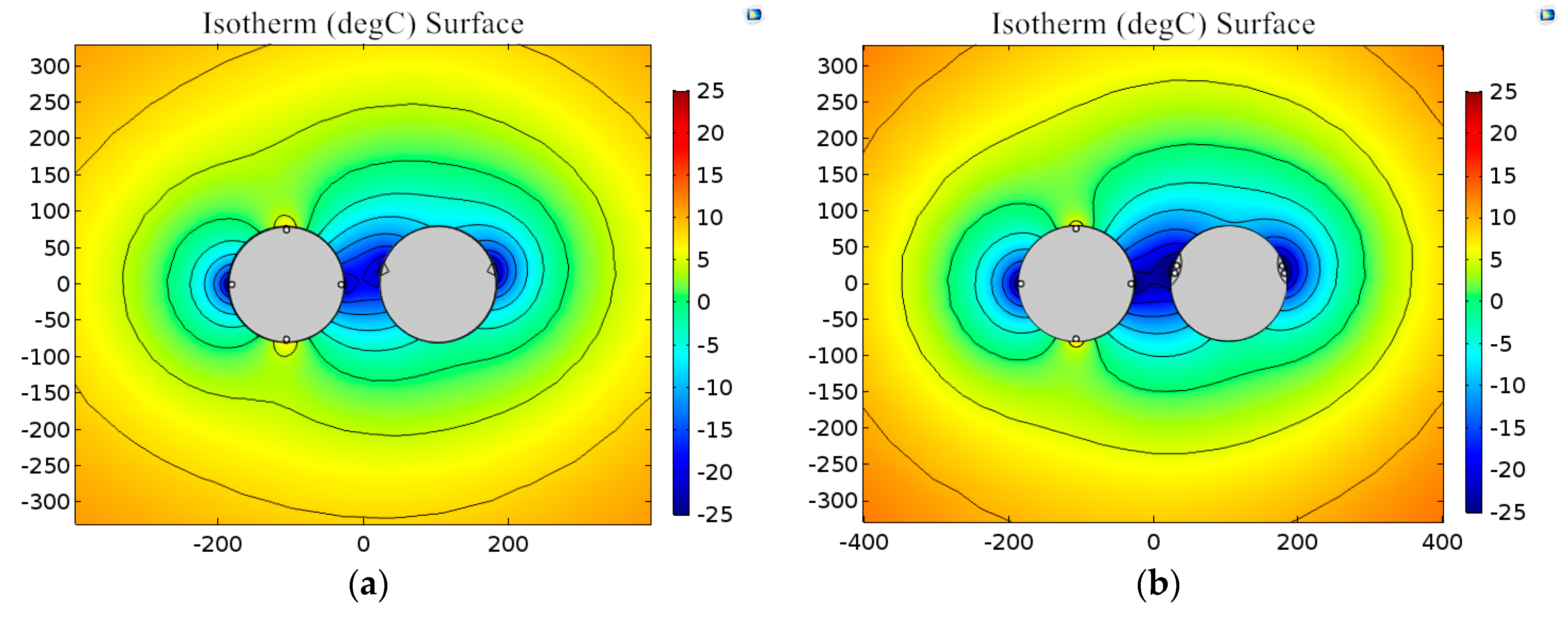
Figure 23.
Average thickness of frozen soil wall in different positions after 42 h.

Table 1.
Dimensions of Pipe and Freezing-Tube.
| Components | Prototype Dimension (mm) | Model Dimension (mm) |
|---|---|---|
| Concrete pipe & hollow pipe (Diameter) | 1600 | 160 |
| Main freezing-tube (Diameter) | 80 | 8 |
| Profiled freezing-tube (Equilateral angle steel) | 125125 | 12.512.5 |
| Limiting-tube (Diameter) | 80 | 8 |
Table 2.
Velocity Parameters.
| Parameter | Prototype Velocity Parameter (Single Tube) | Model Velocity Parameter (Single Tube) |
|---|---|---|
| Tube diameter (mm) | 80 | 8 |
| Rate of flow (m3/h) | 5 | 0.5 |
| Velocity of flow (m/min) | 16.58 | 165.8 |
Table 3.
Properties of the Test Soil.
| Test Soil | Saturated Moisture (%) | Density (g·cm−3) | Thermal Capacity (kJ·kg−1·°C−1) | Thermal Conductivity (W·m−1·K−1) | Freezing Temperature (°C) | |
|---|---|---|---|---|---|---|
| ρ | ρd | |||||
| Saturated sand | 40.29 | 1.435 | 1.317 | 1.372 | 1.475 | −0.5 |
Table 4.
Initial Temperatures before Test.
| Testing Time | Environment Average Temperature (°C) | Average Temperature of Saltwater in Freezing Tube (°C) | Average Temperature of hot Saltwater in Limiting-Tube (°C) | Initial Average Temperature of the Soil (°C) | ||
|---|---|---|---|---|---|---|
| Centerline of the Pipes | Vertical Axis of the Hollow Pipe | Horizontal Axis of the Hollow Pipe | ||||
| 3:30 pm, Apr.30 | 26 | −25 | 9 | 20.2 | 18.7 | 18.4 |
Table 5.
Comparison of temperature data of centerline points 50 mm away from the contour line.
| Measurement Point | t21 (°C) |
Δt21 (°C) | t42 (°C) |
Δt24 (°C) | V1 (°C/h) | V2 (°C/h) | Time of Temperature Below Freezing Point (h) | Δh (h) |
|---|---|---|---|---|---|---|---|---|
| m2 | −0.6 | −4.4 | −1.6 | −2.1 | −0.97 | −0.05 | 21 | −9 |
| m2* | −5 | −3.7 | −1.30 | 0.06 | 12 | |||
| m6 | −0.7 | −3.1 | −1.4 | −1.7 | −1.03 | −0.03 | 21 | −7 |
| m6* | −3.8 | −3.1 | −1.21 | 0.03 | 14 |
Table 6.
Comparison of temperature data of vertical points 50 mm away from the hollow pipe wall.
| Measurement Point | t21 (°C) |
Δt21 (°C) | t42 (°C) |
Δt24 (°C) | V1 (°C/h) | V2 (°C/h) | Time of Temperature Below Freezing Point (h) | Δh (h) |
|---|---|---|---|---|---|---|---|---|
| v2 | 0.5 | −5.3 | −2.3 | −4.4 | −0.85 | −0.13 | 26 | −14 |
| v2* | −4.8 | −6.7 | −1.14 | −0.09 | 12 | |||
| v6 | 1.3 | −4.0 | −1.3 | −3.4 | −0.79 | −0.12 | 33 | −17 |
| v6* | −2.7 | −4.7 | −1.06 | −0.10 | 16 |
Table 7.
Comparison of temperature data of horizontal points of the hollow pipe.
| Measurement Point | t21 (°C) |
Δt21 (°C) | t42 (°C) |
Δt24 (°C) | V1 (°C/h) | V2 (°C/h) | Time of Temperature Below Freezing Point (h) | Δh (h) |
|---|---|---|---|---|---|---|---|---|
| h2 | −1.2 | −3 | −4.2 | −2.6 | −1.00 | −0.14 | 19 | −9 |
| h2* | −4.2 | −6.8 | −1.13 | −0.12 | 10 | |||
| h3 | 4.7 | −3.4 | 0.7 | −2.9 | −0.7 | −0.19 | — | — |
| h3* | 1.3 | −2.2 | −0.97 | −0.16 | 30 |
Table 8.
Thermo-physical properties of materials.
| Materials | Density (kg·m-3) | Thermal Capacity (J·kg-1·K) | Thermal Conductivity (W·m-1·K-1) | Freezing Point (°C) | |||
|---|---|---|---|---|---|---|---|
| Soil | ρ | ρsat | unfrozen | frozen | unfrozen | frozen | −0.5 |
| 1435 | 2055.1 | 1372 | 1071 | 1.475 | 1.795 | ||
| Concrete | 2450 | 920 | 1.95 | - | |||
| Steel pipe | 7850 | 318 | 60 | - | |||
| Cement mortar | 1900 | 840 | 1.28 | - | |||
| Air | 1.29 | 1005 | 0.02 | - | |||
© 2020 by the authors. Licensee MDPI, Basel, Switzerland. This article is an open access article distributed under the terms and conditions of the Creative Commons Attribution (CC BY) license (http://creativecommons.org/licenses/by/4.0/).
Share and Cite
MDPI and ACS Style
Duan, Y.; Rong, C.; Cheng, H.; Cai, H.; Wang, Z.; Yao, Z. Experimental and Numerical Investigation on Improved Design for Profiled Freezing-tube of FSPR. Processes 2020, 8, 992. https://doi.org/10.3390/pr8080992
AMA Style
Duan Y, Rong C, Cheng H, Cai H, Wang Z, Yao Z. Experimental and Numerical Investigation on Improved Design for Profiled Freezing-tube of FSPR. Processes. 2020; 8(8):992. https://doi.org/10.3390/pr8080992
Chicago/Turabian StyleDuan, Yin, Chuanxin Rong, Hua Cheng, Haibing Cai, Zongjin Wang, and Zhishu Yao. 2020. "Experimental and Numerical Investigation on Improved Design for Profiled Freezing-tube of FSPR" Processes 8, no. 8: 992. https://doi.org/10.3390/pr8080992
Note that from the first issue of 2016, this journal uses article numbers instead of page numbers. See further details here.