Numerical Study of Effect of Sawtooth Riblets on Low-Reynolds-Number Airfoil Flow Characteristic and Aerodynamic Performance

Abstract

Riblets with an appropriate size can effectively restrain turbulent boundary layer thickness and reduce viscous drag, but the effects of riblets strongly depend on the appearance of the fabric that is to be applied and its operating conditions. In this study, in order to improve the aerodynamic performance of a low-pressure fan by using riblet technology, sawtooth riblets on NACA4412 airfoil are examined at the low Reynolds number of 1 × 10⁵, and the airfoil is operated at angles of attack (AOAs) ranging from approximately 0° to 12°. The numerical simulation is carried out by employing the SST k–ω turbulence model through the Ansys Fluent, and the effects of the riblets’ length and height on aerodynamic performance and flow characteristics of the airfoil are investigated. The results indicate that the amount of drag reduction varies greatly with riblet length and height and the AOA of airfoil flow. By contrast, the riblets are detrimental to the airfoil in some cases. The most effective riblet length is found to be a length of 0.8 chord, which increases the lift and reduces the drag under whole AOA conditions, and the maximum improvements in both are 17.46% and 15.04%, respectively. The most effective height for the riblet with the length of 0.5 chord is 0.6 mm. This also improves the aerodynamic performance and achieves a change rate of 12.67% and 14.8% in the lift and drag coefficients, respectively. In addition, the riblets facilitate a greater improvement in airfoil at larger AOAs. The flow fields demonstrate that the riblets with a drag reduction effect form “the antifriction-bearing” structure near the airfoil surface and effectively restrain the trailing separation vortex. The ultimate cause of the riblet drag reduction effect is the velocity gradient at the bottom of the boundary layers being increased by the riblets, which results in a decrease in boundary thickness and energy loss.

1. Introduction

Since Walsh [1] and his team took the lead in the study of sharkskin and applied its surface structure to plates in the 1970s, many scholars have studied riblets, which are bionic surfaces, over the last several decades. Nowadays, riblets are applied to surfaces in fluid engineering, such as on aircraft wings, wind turbine blades, and boat surfaces [2]. The most famous application in fluid engineering is the sharkskin swimming suit, which effectively reduces water resistance and increases swimming speed by 3~7.5%.

The research addressing riblets on flat plates provides a basis for the exploration of the appropriate shape and drag-reducing properties of riblets [3,4,5]. Gregory D. et al. [6], and Bechert et al. [7], experimentally investigated different shapes of riblets. The thin blade, sawtooth, scalloped cross-sections, and sharkskin-shape riblets were arranged on a flat plate in an open channel. An improvement in drag reduction of 6% and 7% was achieved by sawtooth riblets and scalloped riblets, respectively. Hou et al. [8], measured the three-dimensional (3D) turbulence over trapezoidal riblets and observed a skin friction reduction of 6.1%. J. H. et al. [9], also compared the flow fields of the V-shaped and thin blade riblets using the direct numerical simulation method. The thin blade riblets were found to produce a higher skin friction drag reduction than that of the V-shape riblets by 3%. The size and arrangement of riblets also affect drag reduction efficiency. O.A. et al. [10], discussed the drag reduction capacity of thin rectangular riblets with different spacing. The maximum drag reduction occurred with a spacing of 18 viscous units. Suzuki Y. et al. [11], demonstrated that the larger the size of riblet, the more pronounced the skin friction of the plate. Moreover, Yulia P. et al. [12], and Sasamori M. et al. [13,14], evaluated the drag reduction effect of the surface of sinusoidal riblets. Via research on flat plates, scholars found that the drag reduction of riblets is achieved by reducing the intensity of the turbulent boundary layer and the amplitude of Reynolds shear stress and vorticity fluctuations [15,16].

The studies on flat plates provide a clear understanding of the drag reduction characteristics and mechanisms of riblets. However, as the flow characteristics of the plate are relatively simple and different from the actual flow, it is inappropriate to directly apply the conclusions of plate flow studies to actual complex flow. Therefore, researchers have begun to investigate how riblets affect the fluid and aerodynamic performance of airfoil. A widely tested airfoil with riblets is the standard airfoil designed by the National Advisory Committee for Aeronautics (NACA) called NACA0012 [17]. Han [18], tested riblets on the NACA0012 at a Reynolds number of 36,000 and observed a drag reduction of 16%. In addition, the airfoil that is common in wind turbine blades has also been arranged with riblets by researchers. Chamorro et al. [19], covered V-shaped riblets on the airfoil section of a full-scale 2.5 MW wind turbine and produced a roughly 6% reduction in airfoil drag. Agrim et al. [20], tested DU 96-W-180 airfoil with four different symmetrical V-shaped riblets. The best configuration significantly reduced the drag by up to 5%, but some riblets with other sizes increased the airfoil drag. To further understand the drag reduction mechanism of riblets on airfoil, the influence of riblets on the flow structure near the airfoil surface is also the focus of many scholars. Viswanath [21], observed flow features caused by riblets at low speeds and found that riblets were more effective under adverse pressure gradients. Zhang et al. [22], applied the implicit large eddy simulation method to simulate the mean velocity profile, Reynolds shear stress, etc. around the airfoil. The results illustrated that the riblets thinned the boundary layer, and the vortex structures were also weakened.

With riblet technology being increasingly applied to fluid engineering, riblets are expected to be arranged on the blade surface of low-pressure fans. Wang et al. [23], simulated the drag reduction capacity of riblets on the airfoil of a centrifugal fan blade and obtained a maximum value of 9.65%. Wu et al. [24], placed riblets on the blade surface of a centrifugal fan and found that the total pressure of the fan with appropriate riblets is higher than that of the original fan. However, low-pressure fans usually operate in a wide variety of conditions. The flow angle of the blades significantly changes when the working operation deviates from the design condition. Therefore, the research conclusions of airfoil riblets mentioned above may no longer be applicable, or they may need to be reconsidered. Consequently, a discussion of the influence of the sizes and placements of riblets on airfoil flow and resistance under different AOA conditions is important.

In this study, the effects of riblets on the resistance of NACA4412 are analyzed. NACA4412 is an asymmetric airfoil; its shape and thickness distributions are similar to those of the elementary stage of fan blades. In addition, the Reynolds number of the airfoil flow is $1\times {10}^5$, under which the blades of low-pressure fans usually operate. Referred to the study conducted by O.A. et al. [10], and those on fans in references [23,24], the sawtooth riblets in the current study are arranged in the airfoil suction surface (SS). The airfoil applying riblets with different lengths and groove widths are meshed by self-coded algebraic grids, and the corresponding flow fields are calculated by steady numerical simulation. The effect of riblets and their mechanisms on aerodynamic performance at various angles of attack (AOAs) are also analyzed in detail.

2. Computational Method

2.1. Problem Definition

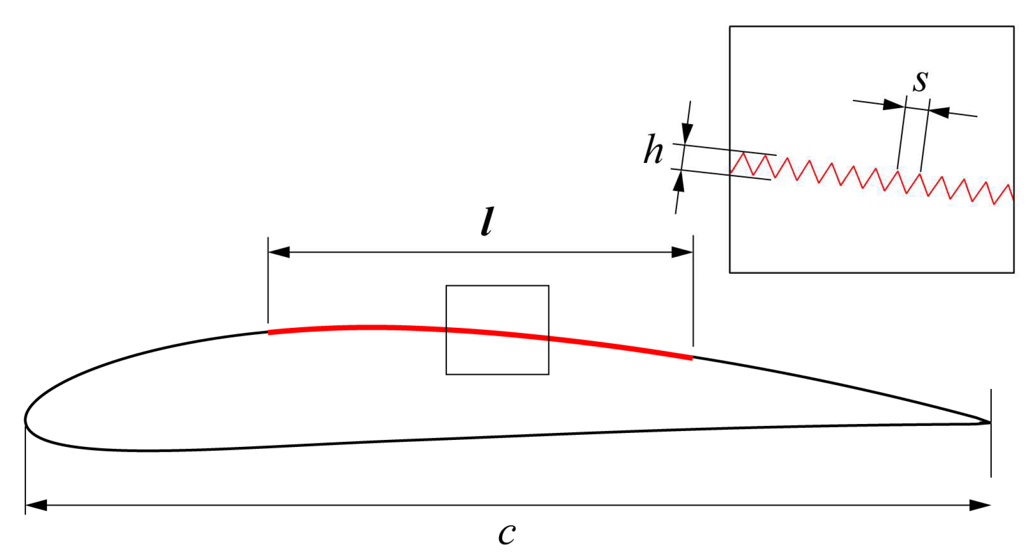
The Reynolds number reflects the effect of inertial force and viscous force on a fluid, which makes the flow present distinct flow characteristics under various operating conditions. With the wide use of low-pressure fans in daily life in both homes and industry, low Reynolds number flow is gradually playing a more critical role. The airfoil is the most essential structure of the fan blade, whose aerodynamic characteristic has a great influence on fan performance. It is important to improve the stability of the airfoil at a low Reynolds number by adopting an optimization strategy.

Considering the fact that the flow angle varies under different working conditions, the turbulent flow over NACA4412 at a 0~12° AOA is considered as the basic flow in this study. The Reynolds number based on the airfoil chord length c and the mean velocity U is $1\times {10}^5$, which is usual in civil-used fans.

The various sawtooth riblets vertical to the flow direction were arranged symmetrically at the middle of the airfoil SS, as shown in Figure 1. The riblets consist of three parameters: their length l, riblet spacing s, and the riblet height h. Numerous studies have shown that the drag can be effectively reduced when s is equal to h [25]. Therefore, the ratio of s and h in this study is set as 1.

2.2. Riblet Design

In this study, we designed sawtooth riblets with various lengths and heights. The cross-sectional shape of the riblets is an isosceles triangle with the apex angle of 53.1°. Michael’s research indicates that riblets with the dimensionless parameters $h^{+}<25$ and $s^{+}<30$ have a certain effect on reducing the friction drag of plates [26]. $h^{+}$ and $s^{+}$ are respectively defined as follows:

$$h^{+}=\frac{h}{K}$$

(1)

$$s^{+}=\frac{s}{K}$$

(2)

where, the dimensionless wall coefficient K is defined as:

$$K=\nu /u_{\tau }$$

(3)

where

$$\nu =\mu /\rho$$

(4)

$$u_{\tau }=\sqrt{{\tau }_w/\rho }$$

(5)

$${\tau }_w=0.0225\rho U^2{\left(\frac{\nu }{U\delta }\right)}^{0.25}$$

(6)

$$\delta =R{e}^{-0.2}$$

(7)

$$Re=\rho Uc/\mu$$

(8)

where $\nu$ is the kinematic viscosity; $u_{\tau }$ is the wall friction velocity; ${\tau }_w$ is the wall shear stress; U is the main flow velocity; c is the chord length of the airfoil; $\mu$ is the dynamic viscosity.

Therefore, the riblet height and spacing can be expressed as

$$h=\frac{h^{+}{c}^{0.875}}{0.15R{e}^{0.9}}$$

(9)

$$s=\frac{s^{+}{c}^{0.875}}{0.15R{e}^{0.9}}$$

(10)

The height of the riblets, whose length varies from $l/c=0.05$ to $l/c=0.8$, is 1 mm; the riblet schemes are named L05~L80, respectively. To gain a further understanding of the relationship between the drag reduction and the riblet height on the airfoil, the heights of the riblets with a length of 0.5c are considered as 0.6, 1.5, 3, 4.5, 6.5, 7.5 and 10 mm, and these riblets are named H06~H100, respectively.

2.3. CFD Governing Equations

The CFD simulations are based on two-dimensional steady Reynolds-averaged Navier–Stokes (RANS) calculations. Imcompressive RANS simulations are performed in Ansys fluent to obtain the flow field, whose governing equations are as follows:

$$\frac{\partial \left(\rho u_i\right)}{\partial x_i}=0$$

(11)

$$\frac{\partial \left(\rho u_i\right)}{\partial t}+\frac{\partial }{\partial x_i}\left(\rho u_i{u}_j\right)=-\frac{\partial P}{\partial x_i}+\frac{\partial }{\partial x_j}\left(\mu \frac{\partial u_i}{\partial x_j}-\rho \overline{u_i^{\prime }{u}_j^{\prime }}\right)+S_i$$

(12)

where $u_i$ represents the velocity components that are averaged in the $x_i$ direction; $\rho$, t, $\mu$, and P are the density, time, dynamic viscosity of the fluid, and average pressure, respectively; $-\rho \overline{u_i^{\prime }{u}_j^{\prime }}$ are Reynolds stresses.

To close Equation (12), the $-\rho \overline{u_i^{\prime }{u}_j^{\prime }}$ must be appropriately modelled. A common method employs the Boussinesq hypothesis to relate the Reynolds stresses to the mean velocity gradients:

$$-\rho \overline{u_i^{\prime }{u}_j^{\prime }}={\mu }_t\left(\frac{\partial u_i}{\partial x_j}+\frac{\partial u_j}{\partial x_i}\right)-\frac{2}{3}\left(\rho k+{\mu }_t\frac{\partial u_k}{\partial x_k}\right){\delta }_{ij}$$

(13)

where, ${\mu }_t$ is the turbulent viscosity, ${\delta }_{ij}$ is the “Kronecker delta” operator.

For determining the ${\mu }_t$, the RANS model can be divided into zero equation model, one equation model and two equation model according to the number of additional transport equation. The two-equation model is the most widely used in engineering simulation comparing with the other equation models.

The shear stress transport k–ω model [27,28] is developed by coupling high Reynolds number $\mathrm{k}\text{–}\mathsf{\epsilon }$ model on the basis of the Wilcox’s $\mathrm{k}\text{–}\mathsf{\omega }$ model. The additional transport equations for the turbulence kinetic energy (k) and the specific dissipation rate (ω) are as follows:

$$\frac{\partial }{\partial t}\left(\rho k\right)+\frac{\partial }{\partial x_i}\left(\rho k{u}_i\right)=\frac{\partial }{\partial x_j}\left({\Gamma }_k\frac{\partial }{\partial x_j}\right)+G_k-Y_k+S_k$$

(14)

$$\frac{\partial }{\partial t}\left(\rho \omega \right)+\frac{\partial }{\partial x_i}\left(\rho \omega u_j\right)=\frac{\partial }{\partial x_j}\left({\Gamma }_{\omega }\frac{\partial \omega }{\partial x_j}\right)+G_{\omega }-Y_{\omega }+S_{\omega }+D_{\omega }$$

(15)

where, $G_k$,$G_{\omega }$ is the generation term of k and ω; ${\Gamma }_k$, ${\Gamma }_{\omega }$ are the effective diffusion terms of k and ω; $Y_k$, $Y_{\omega }$ are the dissipation terms of k and ω; $S_k$, $S_{\omega }$ are the self-defined source terms; $D_{\omega }$ is the cross-diffusion factor.

$${\Gamma }_k=\mu +\frac{{\mu }_t}{{\sigma }_k}, {\Gamma }_{\omega }=\mu +\frac{{\mu }_t}{{\sigma }_{\omega }}$$

(16)

$$Y_k=\rho {\beta }^{*}k\omega , Y_{\omega }=\rho {\beta }^{*}{\omega }^2$$

(17)

$$D_{\omega }=2\left(1-F_1\right)\rho \frac{1}{\omega {\sigma }_{\omega ,2}}\frac{\partial k}{\partial x_j}\frac{\partial \omega }{\partial x_j}$$

(18)

The turbulent viscosity ${\mu }_t$ is computed as follows:

$${\mu }_t=\frac{\rho k}{\omega }\frac{1}{\max \left[\frac{1}{a^{*}},\frac{S{F}_2}{a_1\omega }\right]}$$

(19)

where, S is the strain rate magnitude.

The SST $\mathrm{k}–\mathsf{\omega }$ model combines the advantages of the $\mathrm{k}–\mathsf{\epsilon }$ model and $\mathrm{k}–\mathsf{\omega }$ model. The $\mathrm{k}–\mathsf{\omega }$ model is adopted near the wall while using $\mathrm{k}–\mathsf{\epsilon }$ model at the location far away from the wall. The transition between them is through hybrid functions:

$$F_1=\tanh \left\{{\left\{\min \left[\max \left(\frac{\sqrt{k}}{0.09\omega y},\frac{500\mu }{\rho y^2\omega }\right),\frac{4\rho k}{{\sigma }_{\omega ,2}{D}_{\omega }^{+}{y}^2}\right]\right\}}^4\right\}$$

(20)

$$F_2=\tanh \left\{{\left[\max \left(\frac{2\sqrt{k}}{0.09\omega y},\frac{500\mu }{\rho y^2\omega }\right)\right]}^2\right\}$$

(21)

$$D_{\omega }^{+}=\max \left[2\rho \frac{1}{{\sigma }_{\omega ,2}}\frac{1}{\omega }\frac{\partial k}{\partial x_j}\frac{\partial \omega }{\partial x_j},{10}^{-10}\right]$$

(22)

The rest coefficients ${\sigma }_k$, ${\sigma }_{\omega }$, $\beta$ are calculated by the coefficient ${\varphi }_1$ of $\mathrm{k}–\mathsf{\omega }$ model and the coefficient ${\varphi }_2$:

$$\varphi =F_1{\varphi }_1+\left(1-F_1\right){\varphi }_2$$

(23)

The constants of SST k–ω model are as follows:

• ${\sigma }_{k,1}=1.176,{\sigma }_{\omega ,1}=1.176,{\sigma }_{k,2}=1.0,{\sigma }_{\omega ,2}=1.168$
• $a_1=0.31,{\beta }_{i,1}=0.075,{\beta }_{i,2}=0.0828$

The SIMPLE algorithm is used to perform the pressure–velocity coupling. The second-order upwind discretization and the central difference schemes are adopted for the convection and diffusion terms, respectively. The non-slip wall condition is adopted on the airfoil.

The SIMPLE algorithm is used to perform pressure–velocity coupling. The second-order upwind discretization and the central difference schemes are adopted for the convection and diffusion terms, respectively. The non-slip wall condition is adopted on the airfoil.

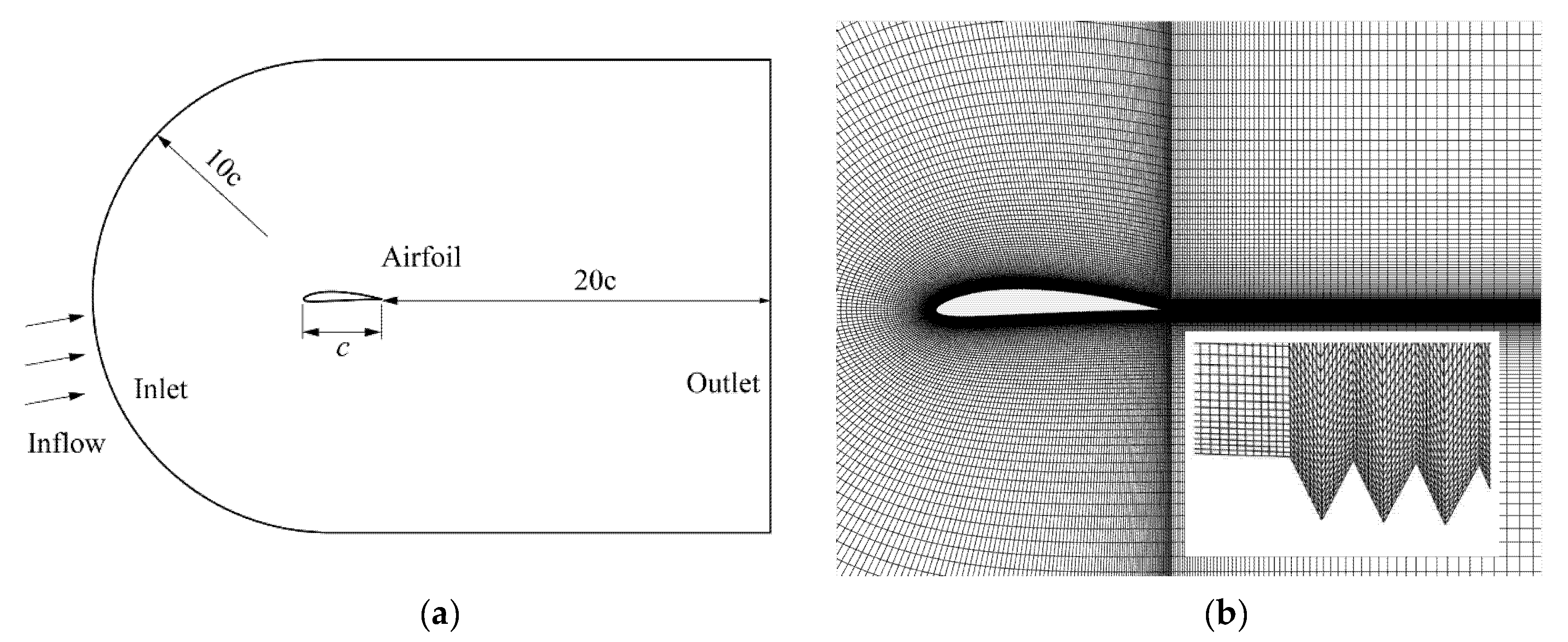
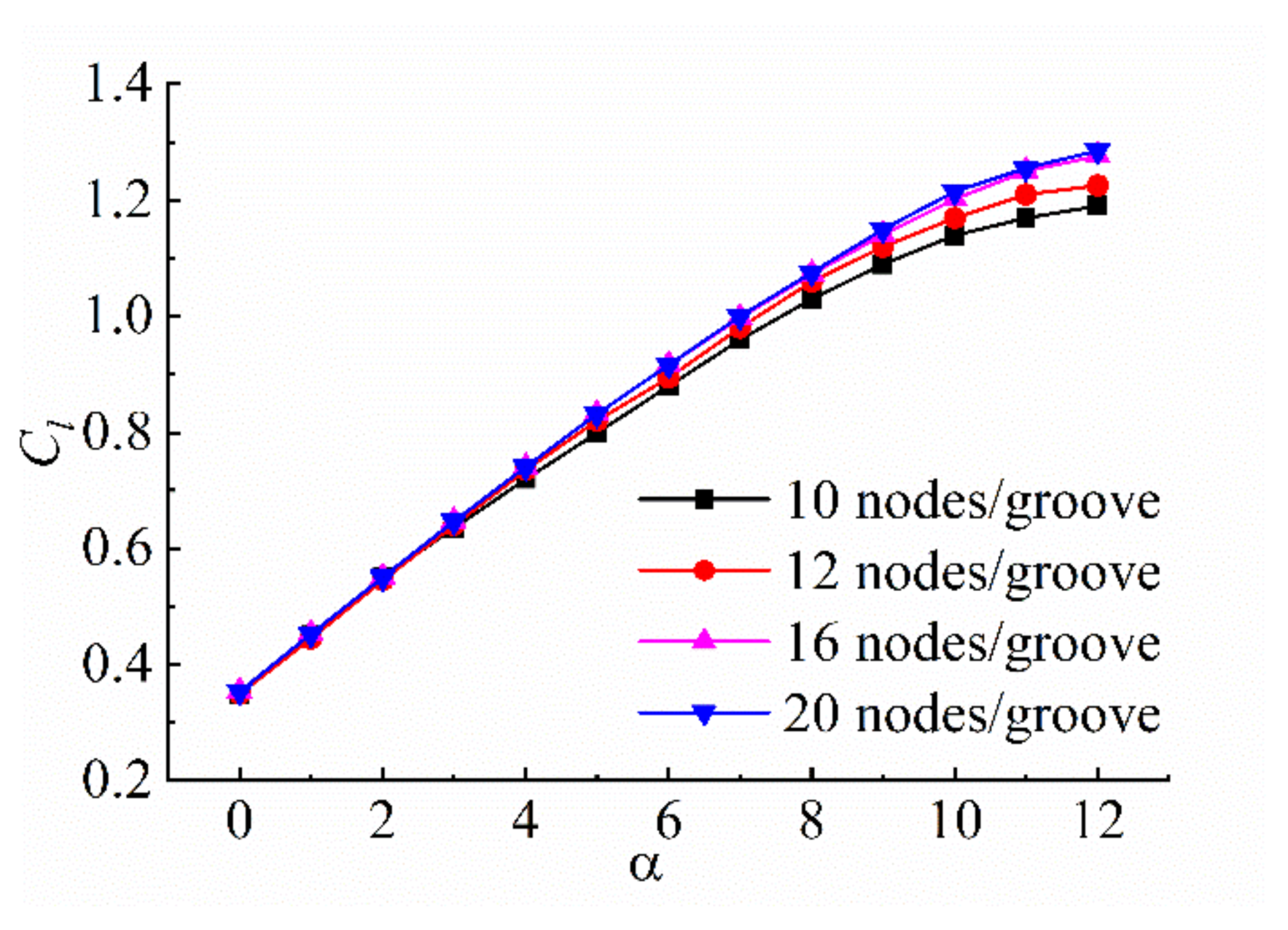
2.4. Mesh Model and Validation

The baseline C-type algebraic meshes generated by the Hermite interpolation function are carried out. The schematic view of flow around the airfoil and the mesh distribution are shown in Figure 2a. The inlet of the computational domain is a semicircle, which is 10c to the airfoil trailing edge (TE), and the outlet is 20c to the airfoil TE. Here, c is the airfoil chord length and is equal to 1 m. The inlet and outlet boundaries are set as the velocity inlet and pressure outlet, respectively. The fluid density is $\rho =1.0 {\mathrm{kg}/\mathrm{m}}^3$, and the dynamic viscosity is $\mu =1\times {10}^{-4} \mathrm{Pa}·\mathrm{s}$. The velocity of the freestream flow is $U=10 \mathrm{m}/\mathrm{s}$, and the Reynolds number based on the main flow velocity is $1\times {10}^5$.

The lift coefficient and drag coefficient are defined as:

$$\begin{gathered} C_l=2F_l/\left(\rho U^{2}c\right) \\ {C}_d=2F_d/\left(\rho U^{2}c\right) \end{gathered}$$

(24)

where $F_l$ and $F_d$ are the lift and drag of the airfoil, respectively.

Four different grid models with increasing grid quantity are built and simulated via three kinds of two equation turbulence models in order to verify the accuracy of the SST $\mathrm{k}–\mathsf{\omega }$ model and the grid convergence. The grid node in the streamwise direction increases from 335 to 793, while the node increases from 101 to 561 in the wall-normal direction. The minimum grid spacing on the airfoil is 0.0002c, located at both the airfoil leading edge (LE) and TE. The first layer height is controlled at 0.00005c to ensure that the first y+ is less than 1. The grid spacing growth rate decreases from 1.15 for the coarsest mesh to 1.03 for the finest one.

Table 1. Lift coefficient comparison of the different turbulence models and grid numbers at various AOAs.

Turbulence Model	Grid Number	0°	4.5°	8°	12°	16°
$\mathrm{RNG}\mathrm{k}–\mathsf{\epsilon }$	$101\times 335$	0.3998	0.8772	1.2003	1.5245	1.7064
	$181\times 441$	0.4024	0.8813	1.2294	1.5379	1.6731
	$271\times 563$	0.4080	0.8855	1.2356	1.5467	1.6617
	$361\times 679$	0.4091	0.8886	1.2398	1.5549	1.6584
$\mathrm{Standard}\mathrm{k}–\mathsf{\omega }$	$101\times 335$	0.4009	0.8793	1.2053	1.5347	1.7099
	$181\times 441$	0.4079	0.8826	1.2327	1.5648	1.6648
	$271\times 563$	0.4126	0.8877	1.2400	1.5690	1.6561
	$361\times 679$	0.4142	0.8905	1.2436	1.5731	1.6519
$\mathrm{SST}\mathrm{k}–\mathsf{\omega }$	$101\times 335$	0.4169	0.8834	1.2115	1.5372	1.7123
	$181\times 441$	0.4213	0.8994	1.2499	1.5733	1.6540
	$271\times 563$	0.4261	0.9036	1.2450	1.5763	1.6470
	$361\times 679$	0.4272	0.9006	1.2435	1.5774	1.6461
Experiment	-	0.4299	0.8959	1.2896	1.6109	1.6120

provides the lift coefficients of the four grids achieved by three turbulence models at different AOAs as well as the experiment data measured by Coles D. and Wadcock A.J. [29]. For the same grid scheme, it can be seen that the lift coefficients solved by the SST $\mathrm{k}–\mathsf{\omega }$ model are closest to the results of the experiment data, and those of the renormalization group $\mathrm{k}–\mathsf{\epsilon }$ model are the worst. Therefore, the $\mathrm{SST}\mathrm{k}–\mathsf{\omega }$ model is sufficiently accurate to solve the two-dimensional flow field of the airfoil.

Except for the results of the coarsest grids ($101\times 335$), the lift coefficients of the other three grid schemes are close to the experimental data at small AOAs. However, the difference between the simulation data and experimental data grows with the increase in the AOA. Figure 3 shows the error between the calculated results of the different grid numbers and experiment values at two AOAs. As the grid number increases, the error continuously decreases. When the grid number exceeds 271 × 563, the deviation can be controlled within 3.4%. However, there is no significant improvement in the prediction accuracy of the lift coefficients when the grid number further increases. As a result, the SST $\mathrm{k}–\mathsf{\omega }$ model and the grid number of 271 × 563 are finally considered as the turbulence model and the mesh model in this study.

Although riblets are microstructures as compared to the entire airfoil, they significantly affect the flow characteristics of airfoil. Therefore, the grid independence of the riblets was also tested based on the grid validation method mentioned above in order to accurately simulate flow field details. That is, the grid number in the riblet was different, while that in the rest of the computational domain was $271\times \left(563-\lfloor 282l/c\rfloor \right)$. l is the length of the riblets on the airfoil. For the riblets with a length $l=0.2c$ and height h of 1 mm, the gird number of each riblet was determined to be 10, 12, 16, or 20. The lift coefficients of different grid schemes at various AOAs were calculated numerically at the Reynolds number of $1\times {10}^5$. Figure 4 shows that the lift coefficients of each scheme are basically identical at small AOAs, and the tendency is consistent. However, the difference grows with the increase in the AOA. When the grid number in each riblet reaches 16 or 20, the lift coefficient remains unchanged, indicating that the riblet grid number is sufficient. Therefore, the grid number on the single riblet is 16, as $h=1 \mathrm{mm}$, and it increases in equal proportion to the enlargement in h. Thus, to ensure the same grid topology and grid density, the grid numbers of the two-dimensional calculation model are 271 × 563 (original airfoil) and $271\times \left(563-\lfloor 282l/c\rfloor +16n\right)$, where n is the riblet number for various schemes.

3. Result, Analysis, and Discussion

The numerical results of the original airfoil and that with the various riblets are compared in this section. The freestream conditions of all cases are based on the $1\times {10}^5$ Reynolds number and a 0~12° AOA.

3.1. Flow Characteristics of the Riblets Inside the Boundary Layer

As several kinds of riblets with different lengths are designed in this section, the L70 scheme is taken as an example to explore the influence of the riblets on the flow characteristics inside the airfoil boundary layer.

Table 2. Change rate of the aerodynamic performance of the L70 scheme at various AOAs.

AOA	$\Delta {\mathit{C}}_{\mathit{l}} (\%)$	$\Delta {\mathit{C}}_{\mathit{d}} (\%)$	$\Delta {\mathit{C}}_{\mathit{l}}/{\mathit{C}}_{\mathit{d}} (\%)$
0	7.610	−0.293	7.926
2	6.383	−1.160	7.632
4	5.798	−1.953	7.906
6	5.478	−2.537	8.224
8	6.121	−4.081	10.636
10	8.852	−8.466	18.920
12	15.778	−15.369	36.803

shows the change in the aerodynamic performance induced by the L70 scheme at several AOAs. The amelioration of the lift coefficient and the ratio of lift to drag are significant. Although the improvement in the drag coefficient is slight at a 0° AOA, it increases as the AOA grows.

Figure 5 compares the velocity profiles of the streamwise locations among the four schemes at a 12° AOA from $x/c=0.1$ to $x/c=0.8$. The abscissa is the non-dimensional velocity at the assigned location, and the ordinate y is the wall-normal distance from the airfoil wall. The leading separation vortex (LSV) and the trailing separation vortex (TSV) of the original are clear at $x/c=0.1$ and $x/c=0.6~0.8$, as the non-dimensional velocity is negative at the valley of the boundary layer.

Due to the advanced LSVs of the three riblet schemes, their non-dimensional velocities at $x/c=0.1$ are also negative. At $x/c=0.2~0.4$, the velocity distributions of the riblet schemes closely resemble that of the original. However, the velocity distribution changes greatly after $x/c=0.5$ because of the different TSVs formed in the four schemes. The L50 and L70 schemes basically eliminate the negative velocity gradient at the boundary layer valley, while it is also relieved by the L20 scheme. Within the boundary layer, the velocity gradient of the riblet schemes is higher than that of the original, resulting in a reduction in the boundary layer thickness. Therefore, the momentum and energy loss in the boundary layer are suppressed by the riblets.

Figure 6 shows the streamlines and pressure contours of the L70 scheme at the different locations of the riblets under the condition of a 12° AOA. The selected riblets are located at the position prior to the TSV, the starting position of the TSV, and the position inside the TSV. The vortex of riblets (VOR) and the minor vortex below the VOR are formed due to the microstructure of the riblets. Before the starting point of the TSV, the VOR is inside the riblet, and the pressure distribution at the riblet peak is the symmetrical sector. When the flow separation arises, the fluid with the inverse velocity increases and flows into the riblet. Therefore, the VOR moves upward and invades the mainstream, contributing to the smaller velocity inside the riblet and the decreased pressure difference at the riblet peak. As the airfoil TSV was adequately developed, the fluid with a reverse velocity gradient occupies most of the riblet, and the VOR is a certain distance away from the riblet. As a result, the pressure difference at the riblet tip is further reduced and forms a symmetrical strip structure. It is noteworthy that the rotational directions of the VORs at the different locations are all in accordance with the main flow. Consequently, the VORs caused by the riblets play the role of the rolling bearings installed on the airfoil surface, reducing the viscous drag of the airfoil.

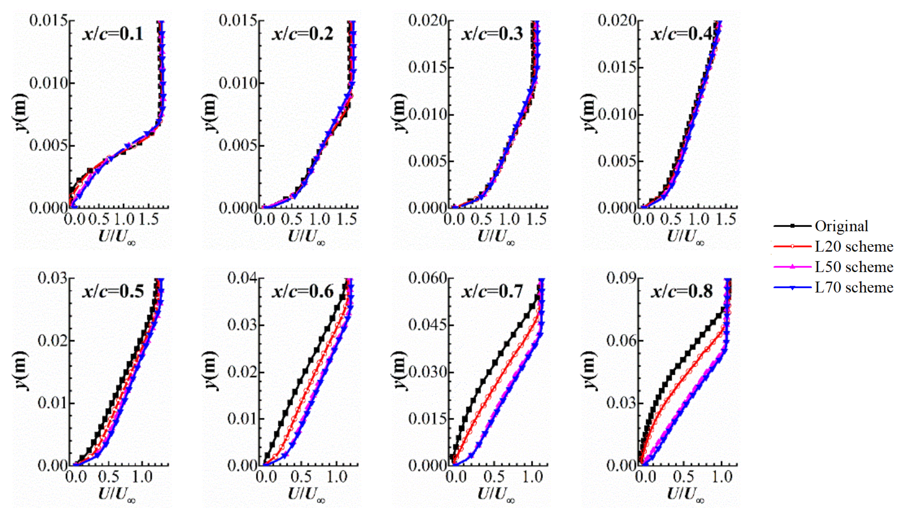
3.2. Effect of the Riblets with Different Lengths

Figure 7 shows the variation in lift and drag coefficients of the configurations with different lengths obtained by surface integration. The lift and drag coefficients are both affected by the various riblets at a 0~12° AOA. The variation in lift coefficients acquired by L05 and L10 schemes is negative at most AOAs, and that of the L10 scheme is the worst. This suggests that a small riblet length is disadvantageous to the airfoil lift coefficient. When the length exceeds 0.2c, the lift coefficient augment is increased with the increase in length. As l reaches 0.8c (L80 scheme), the considerable growth of the maximum lift coefficient is up to 17.46%. Meanwhile, the effect of the riblets on the lift coefficient is also affected by the AOA. When the l of the riblets is between 0.2c and 0.5c, the augmentation of the lift coefficient increases with the increase in the AOA. However, the riblets whose lengths exceed 0.7c perform better at small and large AOAs than at medium AOAs. The minimum improvement is obtained at a 6° AOA.

Figure 7b demonstrates that a portion of the designed riblets with various lengths induces a lower drag coefficient compared to the original airfoil. It is more difficult to decrease the drag coefficient than to increase the lift coefficient for the riblets. The change in the drag reduction is not constant with the riblet length when $l\le 0.1c$, and the drag reduction capacity of scheme L10 is worse than that of scheme L05. As the riblet length exceeds 0.3c, the drag reduction is acquired at the 7~12° AOA, and its change rate increases as the AOA grows. When l is 0.8c, the maximum reduction in the drag coefficient of 15.04% is obtained at 12 degrees. It is clear that the performance of the riblets in decreasing the drag is poor at small AOAs, especially at an AOA of 0~3°. The lower drag can only be induced at a 0~6° AOA by schemes L70 and L80. As a result, when $l\ge 0.2c$, the drag reduction capacity increases with the enlargement of riblet l.

As the airfoil drag is compounded from the viscous drag and pressure drag, the drag coefficient can be expressed by the pressure coefficient and friction coefficient, which is:

$$C_d=C_{d,p}+C_{d,v}=-{\displaystyle \oint C_{p}d{l}_x+{\displaystyle \sum _{i=0}^c{C}_f\sin \phi }}$$

(25)

where $\phi$ is the tangential angle of the airfoil surface. As ${\displaystyle \oint C_{p}d{l}_x}$ is negative, ${\displaystyle \oint C_{p}d{l}_x}$ is marked with a minus to obtain a positive value in order to unify scalars.

Figure 8 shows the drag component changes in the riblets with different lengths. The percentage of the pressure drag in the original drag is positively correlated with the AOA under the whole operating conditions. The viscous drag plays a more critical role than that of the pressure drag at small AOAs, accounting for more than half of the total drag. However, the effect of the drag component is opposite at large AOAs. Therefore, this explains why the performance of the riblets in decreasing the airfoil drag is different at the various AOA. For the L05 scheme, although the riblet raises the pressure drag at most AOAs, the viscous drag is only increased at a 5° AOA, contributing to the total drag of the L05 scheme at the whole range being substantially identical to that of the original. The viscous drag of the L10 scheme increases at a 0~6° AOA and decreases at a 7~12° AOA, while the pressure drag increases under a 0~11° AOA. Consequently, the reduction in the airfoil drag is only induced at a 12° AOA by 1.447%.

It can be seen that the riblets with an appropriate length exert a favorable effect on the viscous drag decrease. When the length of the riblets increases, the viscous drag reduction efficiency is entirely superior. On the contrary, the pressure drag of the riblet schemes is significantly increased, especially at 0~3° AOA, which counteracts the viscous drag decrease at those AOAs. It is mentioned that the pressure drag increment of each riblet scheme is reduced with the enlargement of the AOA. Consequently, the pressure drag of the designed schemes at 10~12° AOA is decreased when $l\ge 0.2c$, resulting in a significant effect on the drag reduction.

The reduction in the pressure drag at 10~12° AOA is mainly caused by the diminishing separation vortex at the airfoil TE. Figure 9 shows the pressure coefficients, the pressure contour, and the streamlines of the original and the three riblet schemes at a 12° AOA. A primarily TSV and a tiny LSV are formed at the original profile, as shown in Figure 9a. When the riblets are arranged at the airfoil surface, the TSVs of the three configurations are significantly reduced. However, the enlarged LSVs are also induced by the designed riblets. It can clearly be seen that the pressure coefficient of the original airfoil has a slight bump at 0.1c~0.13c, corresponding to the LSV. The bumps in the L50 and L70 schemes are larger than those in the original, and their locations move forward, indicating an increase in the LSVs. The pressure coefficients of the riblet schemes on the airfoil SS are lower than those on the original, leading to an increase in the lift coefficients. Moreover, the increment rate of the lift coefficients is relative to the riblet length.

Distinct from the change in the pressure drag at large AOAs, its significate increase at small AOAs is due to the pressure difference at the riblet surface. Figure 10 shows the pressure contours and the streamlines of the original and the L70 schemes at a 0° AOA. No flow separation appears at the original airfoil, and no flow separation is restrained by the riblets. The pressure distribution and the streamline of the L70 scheme are also similar to those of the original. As a result, the pressure drag increases rather than decreasing. Moreover, the pressure difference at each riblet increases. Figure 11 shows the pressure contours of the L20 and L70 schemes at the riblets. The pressure difference of these two schemes riblet at the same location is 0.5 Pa and 0.6 Pa, respectively. Considering the fact that longer riblets contain more riblet structures, the pressure drag of the L70 scheme is much higher than that of the L20 scheme and the original.

As shown in Figure 8a, the reduction in viscous drag is achieved by the riblets with $l\ge 0.2c$ at most AOAs. To understand the cause of the reduction, the wall shear stress (WSS) distributions of the four schemes at the 0.45c~0.564c on airfoil SS with 12° AOA are compared in Figure 12. The WSS changes periodically in every riblet, and the WSS value reaches the maximum at the riblet peak. The peak value is significantly larger than that of the original because of the higher velocity gradient at the location. In contrast, the velocity gradient inside the riblet is lower than that of the original, resulting in a smaller WSS value. Moreover, the WSS near the riblet valley is very close to zero, demonstrating that the fluid is almost static at the valley. The undulant WSS distribution of the riblets was equivalent averaged and is depicted by the dash–dot line in the graphs. It can be seen that the equivalent mean WSS on the riblets at this position is much lower than that of the original due to the small value at the riblet valley.

The influences of the various riblets on the WSS distribution of the airfoil suction surface are compared in Figure 13. For the convenience of comparison, the WSS at the locations with riblets is averaged due to the periodic fluctuation. The WSS of the original airfoil suddenly increases at 0.1c and decreases to nearly 0 at 0.13c, because the LSV appears. With the LSV developed, the inverse velocity gradient increases, thereby increasing the WSS. When the mainstream is reattached to the airfoil surface, the inverse velocity gradient and the WSS gradually decrease to 0, and the positive velocity gradient increases again. At 0.5194c, the original TSV begins to take form and develops until reaching the airfoil TE. Therefore, the WSS decreases to the minimum at 0.5194c and then increases with the development of the inverse velocity gradient.

When the riblets are arranged on the airfoil, a sudden increase in the WSS arises at the starting position of the riblets, and the WSS distribution of each riblet scheme is similar to that of the original. However, the positions of the minimum WSS and the maximum WSS are slightly different on account of the advance and enlargement in the airfoil LSVs. Moreover, the larger LSVs of the riblet schemes are responsible for the higher inverse velocity gradient inside the separation bubbles. As a result of the shorter riblet length and larger WSS at the airfoil LE, the viscous drag of the L20 scheme slightly increases.

When the riblet $l$ exceeds 0.5c, the position and size of the advanced LSVs slightly change, indicating that the influence of riblet $l$ on the airfoil LSV decreases when $l>0.5c$. Although the WSS of the riblet schemes is higher than that of the original at $x<0.13c$, the much lower averaged WSSs at the riblets are obtained by the small WSS value at each riblet valley. Consequently, the reduction in viscous drag is mainly caused by a decrease in the WSS of the riblets, which is more significant when the riblet $l$ is large.

3.3. Effect of Riblets with Different Heights

As the riblets with a length of 0.5c effectively improve the airfoil aerodynamic performance at most AOAs, the riblets with different heights under 0.5c are designed in this section. Figure 14 illustrates the changes in the lift and the drag coefficients caused by the riblet scheme with five different heights. The lift coefficient at each AOA is improved when $h\le 6.5 \mathrm{mm}$, and the increase rate multiplies rapidly after an 8° AOA. However, the capability of the lift increase gradually reduces as h increases, and the lift coefficient of the H100 scheme is less than that of the original at a 0~7° AOA.

The variation law of the drag coefficient with riblet h is similar to that of the lift coefficient. When $h=10 \mathrm{mm}$, the drag coefficient significantly increases at a 0°~10° AOA, and the maximum reaches 9.49% at a 7° AOA. It is worth mentioning that the drag reduction capacity of the riblets at each $h$ is inadequate when the AOA is between 0° and 7°. The drag reduction is inefficient when $h\le 4.5 \mathrm{mm}$, while the drag coefficients are increased by the other schemes.

Table 3. Change in the pressure drag, viscosity drag, and total drag among the various riblet schemes.

Scheme	Pressure Drag (%)	Viscous Drag (%)	Total Drag (%)
H06	6.45	−15.68	−2.37
H15	8.47	−16.70	−1.56
H45	15.35	−20.08	1.23
H65	20.43	−21.42	3.76
H75	23.85	−21.99	5.58
H100	31.17	−22.46	9.80

presents the change in the drag components and the total drag among the six riblet schemes at a 7° AOA. When the fluid passes through the riblet tip, the pressure difference in the riblet increases with the increase in h. This contributes to the notion that the pressure drag of the riblet scheme is greater than that of the original, and its amount is in proportion to the riblet height. By contrast, the value of the viscosity drag decreases with the increase in height, and the reduction rate declines when the size exceeds 4.5 mm. As the pressure drag of the riblet schemes becomes the principal component of the total drag, and the viscous drag reduction is not proportional to the riblet size at larger heights, the drag reduction capability of riblets decreases, and the total drag of the configurations increases.

The pressure coefficients of the riblet schemes and the original at a 7° AOA are compared in Figure 15. The pressure coefficient of the H06 scheme is slightly higher than that of the original, resulting in a greater lift coefficient. Moreover, the pressure coefficient changes periodically in each riblet because of the pressure differences at the riblets’ windward and leeward sides. As the pressure coefficient of the H100 scheme is the same as that of the original at most of the surface, the reduction at 0.25c~0.411c on the SS is the main reason for the decline in the lift coefficient. Therefore, the riblets with an inappropriate height leads to the pressure coefficient being diminished.

The WSSs of the original and the three riblet schemes at 0.45c~0.5c of the airfoil surface are depicted in Figure 16. Due to the different heights of the riblets, the riblet number of the three configurations at the assigned location is 34, 11, and 5. Although the values of the WSS are almost 0 at the riblet valley, the value at the riblet peak varies considerably. As the peak value is determined by the velocity gradient magnitude at the riblet tip, it is in proportion to the riblet height. By contrast, the riblet with a more considerable height is able to accommodate more low-speed airflows, resulting in the lower WSS inside the riblet. Therefore, the riblets with a more significant height have a more specific effect on reducing the viscous drag.

Figure 17 shows the streamlines and pressure distribution of the three schemes in the riblets at the same locations. Because the TSV is not present at this position, the VORs are inside the riblets. It is noteworthy that the cores of the VORs gradually deviate from the riblet center when the riblet height increases. The larger the height of the riblets, the more eccentric the cores of VORs.

The bottom row of Figure 17 shows the pressure distribution at the local riblets. The pressure difference of the riblet raises from 1.2 Pa to 3.8 Pa as the riblet height increases from 0.6 mm to 10 mm, resulting in more considerable pressure drag. Meanwhile, the pressure distribution at the riblet peak is also different. The high-pressure area of the H06 scheme is basically consistent with its low-pressure area, forming a symmetrical distribution at each riblet peak. However, when the height reaches 10 mm, the low-pressure area clearly moves to the windward side of the downstream riblet and squeezes its high-pressure area. Consequently, the VORs’ cores of the H100 scheme are close to the riblet’s windward side.

4. Conclusions

In order to introduce riblets into the blade surface of a low-pressure fan, riblets with multiple lengths and heights are applied to a NACA4412 airfoil at the Reynolds number of $1\times {10}^5$. The influence of various riblets on the airfoil aerodynamic performance and the riblet drag reduction mechanism are numerically studied using the $\mathrm{SST}\mathrm{k}–\mathsf{\omega }$ turbulence model. The following conclusions are obtained:

(1)

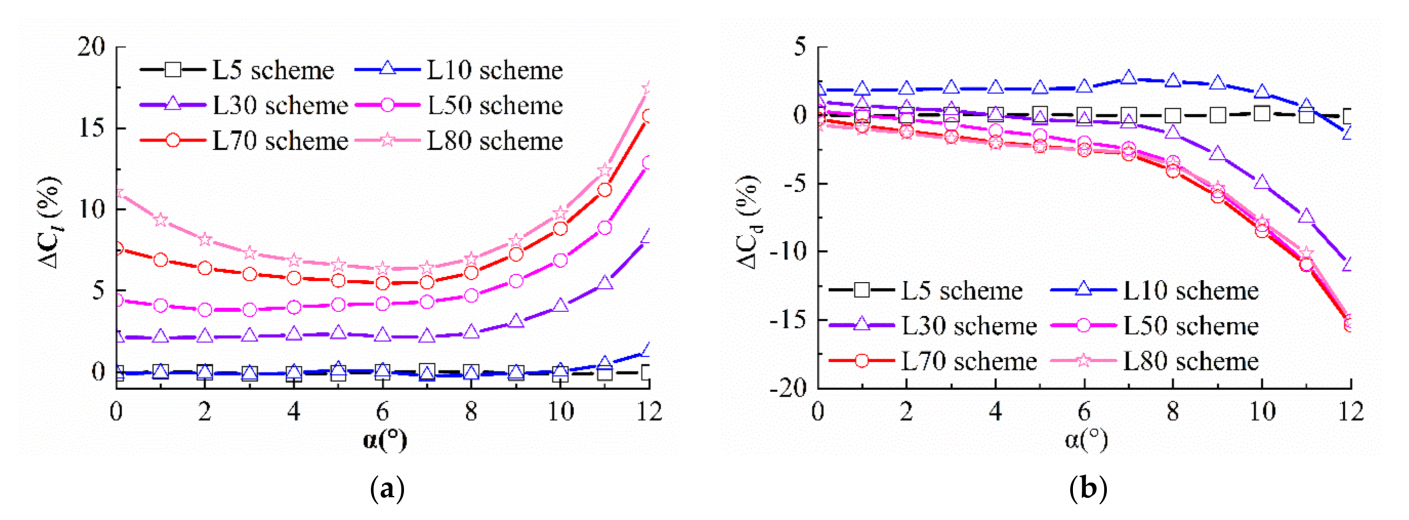
The amount of drag reduction considerably varies with the length and height of the riblet and the AOA of the airfoil flow. When the length exceeds 0.2c, the improvement in the aerodynamic performance is nearly proportional to the riblet length. The most efficient riblet length is found to be 0.8c, which increases the lift and reduces the drag by 17.46% and 15.04% at a 12° AOA, respectively. On the contrary, the riblets with a length of 0.05c and 0.1c are unfavorable to the airfoil.

(2)

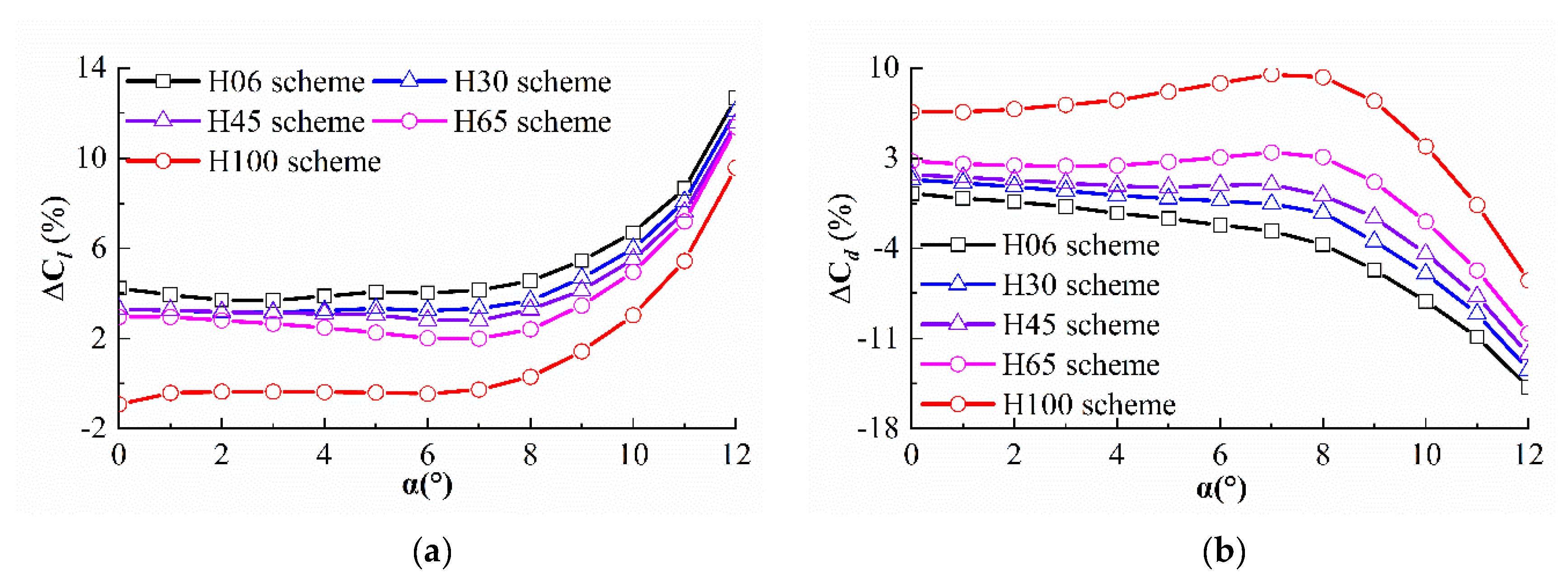
The drag reduction effect is in inverse proportion to the riblet height. The riblets with larger heights the airfoil drag at most of the designed AOAs. The most efficient riblet height in this study is 0.6 mm, as it produces an increase in lift and reduction in drag of 12.67% and 14.8%, respectively. Moreover, the riblets with different sizes perform better at a large AOA than at a small AOA, especially when considering riblet height. The drag coefficients of the riblets whose heights exceed 0.6 mm are significantly increased at a 0~7° AOA.

(3)

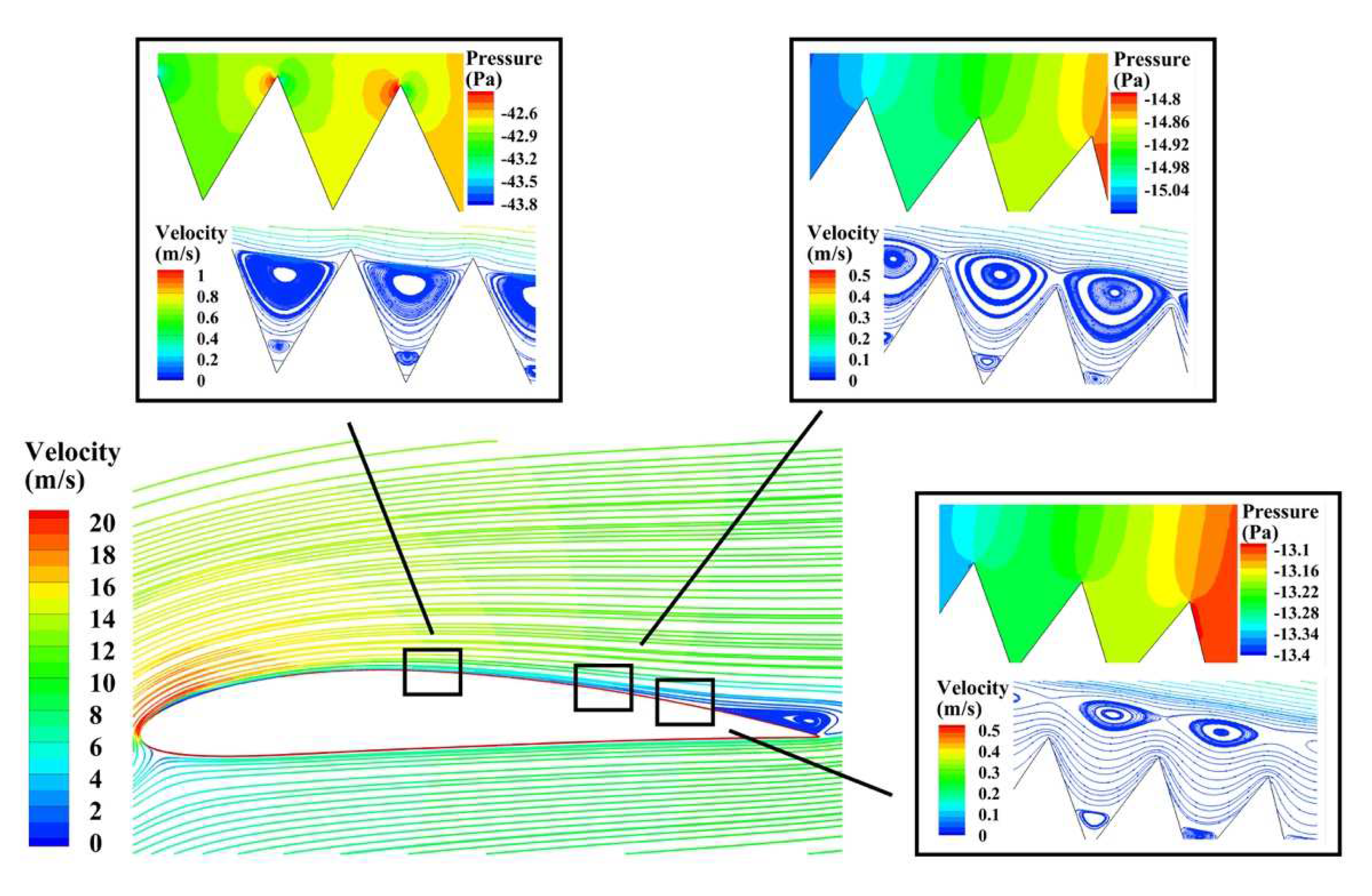
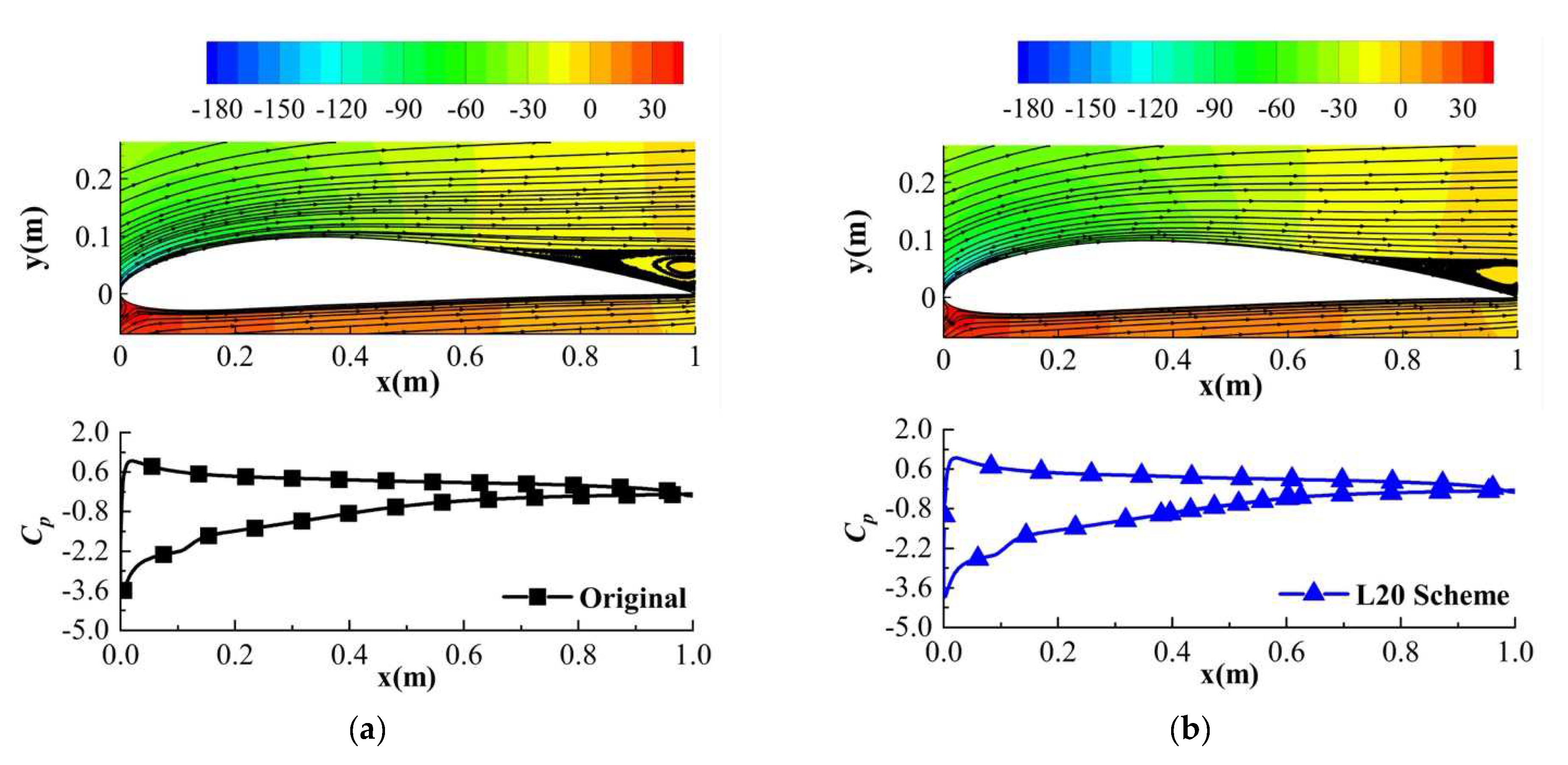
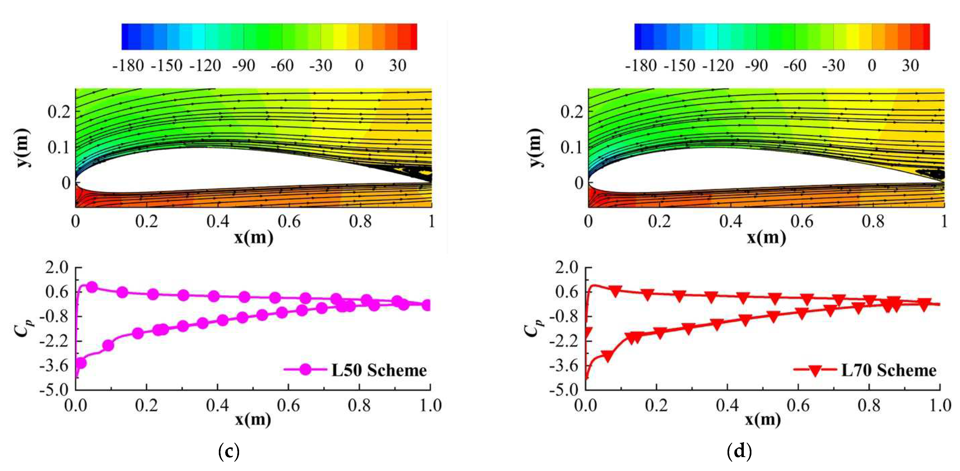
When the flow separation occurs at the airfoil surface, the presence of riblets effectively restrains the trailing edge separation (TSV) compared with the original profile. Nevertheless, no flow separation appears at the small AOA, while the riblets increase the pressure difference at the tip of the structure. The significantly diminished TSV at a large AOA is the main reason for the reduction in the pressure drag, and it explains why the riblets perform better under these conditions.

(4)

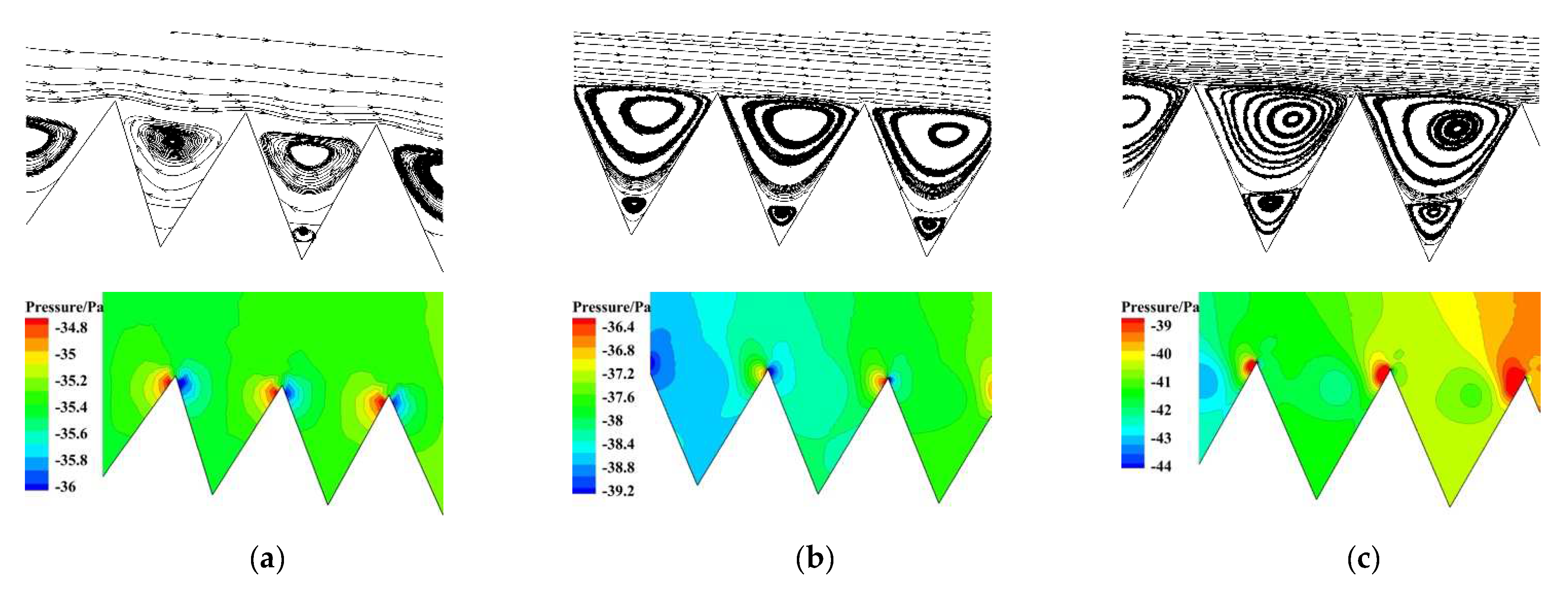
The reason why the riblets decrease the airfoil viscous drag is that the vortex of riblet formed in it plays the role of the rolling bearing. The boundary layer’s thickness, energy loss, and momentum loss are also reduced due to the increase in the velocity gradient at the bottom of the boundary layer.

The influence of riblet size on NACA4412 airfoil is clarified in this study, which provides a reference for the design of riblets on fan blades. Further research is required to determine whether these principles work in the three-dimensional blade. The impact of riblet blades on the fan performance and flow field will be verified in future work.

References

1. Walsh, M.J. Drag Characteristics of V Groove and Transverse Curvature Riblets. In Viscous Flow Drag Reduction; Hough, G.R., Ed.; American Institute of Aeronautics and Astronautics: Dallas, TX, USA, 1980; Volume 72, pp. 168–184. [Google Scholar]
2. Fu, Y.F.; Yuan, C.Q.; Bai, X.Q. Marine drag reduction of shark skin inspired riblet surfaces. Biosurf. Biotribol. 2017, 3, 11–24. [Google Scholar] [CrossRef]
3. Jung, Y.C.; Bhushan, B. Biomimetic Structures for Fluid Drag Reduction in Laminar and Turbulent Flows. J. Phys. Condens. Matter 2010, 22, 35104–35112. [Google Scholar] [CrossRef]
4. Bechert, D.W.; Bruse, M.; Hage, W. Experiments on Drag-Reducing Surfaces and Their Optimization with an Adjustable Geometry. J. Fluid Mech. 1997, 338, 59–87. [Google Scholar] [CrossRef]
5. Bai, X.; Zhang, X.; Yuan, C. Numerical Analysis of Drag Reduction Performance of Different Shaped Riblet Surfaces. Mar. Technol. Soc. J. 2016, 50, 62–72. [Google Scholar] [CrossRef]
6. Bixler, G.D.; Bhushan, B. Fluid Drag Reduction with Shark-Skin Riblet Inspired Microstructured Surfaces. Adv. Funct. Mater. 2013, 23, 4507–4528. [Google Scholar] [CrossRef]
7. Bechert, D.W.; Bruce, M.; Hage, W. Experiments with three-dimensional riblets as an idealized model of shark skin. Exp. Fluids 2000, 28, 403–412. [Google Scholar] [CrossRef]
8. Hou, J.; Vajdi Hokmabad, B.; Ghaemi, S. Three-dimensional measurement of turbulent flow over a riblet surface. Exp. Therm. Fluid Sci. 2017, 85, 229–239. [Google Scholar] [CrossRef]
9. Ng, J.H.; Jaiman, R.K.; Lim, T.T. Direct Numerical Simulations of Riblets in a Fully-Developed Turbulent Channel Flow: Effects of Geometry. In Advances in Computation, Modeling and Control of Transitional and Turbulent Flows; World Scientific: Singapore, 2016. [Google Scholar]
10. El-Samni, O.A.; Chun, H.H.; Yoon, H.S. Drag reduction of turbulent flow over thin rectangular riblets. Int. J. Eng. Sci. 2007, 45, 436–454. [Google Scholar] [CrossRef]
11. Suzuki, Y.; Kasagi, N. Turbulent drag reduction mechanism above a riblet surface. AIAA J. 1994, 32, 1781–1790. [Google Scholar] [CrossRef]
12. Yulia, P.; Pierre, S.; Yves, C. Turbulent Drag Reduction using Sinusoidal Riblets with Triangular Cross-Section. In Proceedings of the 38th AIAA Fluid Dynamics Conference and Exhibit, Seattle, WA, USA, 23–26 June 2008; pp. 2008–3745. [Google Scholar]
13. Sasamori, M.; Mamori, H.; Iwamoto, K. Experimental study on drag-reduction effect due to sinusoidal riblets in turbulent channel flow. Exp. Fluids 2014, 55, 1828. [Google Scholar] [CrossRef]
14. Sasamori, M.; Iihama, O.; Mamori, H. Parametric Study on a Sinusoidal Riblet for Drag Reduction by Direct Numerical Simulation. Flow Turbul. Combust. 2017, 99, 47–69. [Google Scholar] [CrossRef]
15. Goldstein, D.; Handler, R.; Sirovich, L. Direct numerical simulation of turbulent flow over a modeled riblet covered surface. J. Fluid Mech. 1995, 302, 333–376. [Google Scholar] [CrossRef]
16. Choi, H.; Moin, P.; Kim, J. Direct Numerical Simulation of Turbulent Flow Over Riblets. J. Fluid Mech. 1993, 255, 503–509. [Google Scholar] [CrossRef]
17. Caram, J.M.; Ahmed, A. Effect of riblets on turbulence in the wake of an airfoil. AIAA J. 1991, 29, 1769–1770. [Google Scholar] [CrossRef]
18. Han, M.; Lim, H.C.; Jang, Y.G. Fabrication of a Micro-Riblet Film and Drag Reduction Effects on Curved Objects. In Proceedings of the TRANSDUCERS, Solid-State Sensors, Actuators and Microsystems, 12th International Conference on Solid State Sensors, Boston, MA, USA, 8–12 June 2003. [Google Scholar]
19. Chamorro, L.P.; Arndt, R.E.A.; Sotiropoulos, F. Drag reduction of large wind turbine blades through riblets: Evaluation of riblet geometry and application strategies. Renew. Energy 2013, 50, 1095–1105. [Google Scholar] [CrossRef]
20. Sareen, A.; Deters, R.W.; Henry, S.P. Drag Reduction Using Riblet Film Applied to Airfoils for Wind Turbines. J. Sol. Energy Eng. 2013, 136, 021007. [Google Scholar] [CrossRef]
21. Viswanath, P.R. Aircraft viscous drag reduction using riblets. Prog. Aerosp. Sci. 2002, 38, 571–600. [Google Scholar] [CrossRef] [Green Version]
22. Zhang, Y. Numerical study of an airfoil with riblets installed based on large eddy simulation. Aerosp. Sci. Technol. 2018, 78, 661–670. [Google Scholar] [CrossRef]
23. Wang, S.; Rong, R.; Zhengren, W.U. Research on Drag-reduction Characteristic of Non-smooth Surface Riblet Structure on Aerofoil Blade of Centrifugal Fan. Proc. CSEE 2013, 33, 112–118. [Google Scholar]
24. Zhengren, W.U.; Hao, X.; Rong, R. Three-dimensional Numerical Analysis on Drag Reduction Characteristics of the Riblet Structure for Centrifugal Fan Blades. Proc. CSEE 2014, 34, 1815–1821. [Google Scholar]
25. Neumann, D.; Dinkelacker, A. Drag measurements on V-grooved surfaces on a body of revolution in axial flow. Appl. Sci. Res. 1991, 48, 105–114. [Google Scholar] [CrossRef]
26. Walsh, M.J. Riblets as a Viscous Drag Reduction Technique. AIAA J. 1983, 21, 485–486. [Google Scholar] [CrossRef]
27. Li, X.; Li, Z.; Zhu, B.; Wang, W. Effect of Tip Clearance Size on Tubular Turbine Leakage Characteristics. Processes 2021, 9, 1481. [Google Scholar] [CrossRef]
28. Huang, Z.; Shi, G.; Liu, X. Effect of Flow Rate on Turbulence Dissipation Rate Distribution in a Multiphase Pump. Processes 2021, 9, 886. [Google Scholar] [CrossRef]
29. Coles, D.; Wadcock, A.J. Flying-Hot-Wire Study of 2-Dimensional Mean Flow Past an NACA 4412 Airfoil at Maximum Lift. In Proceedings of the 11th Fluid and Plasma Dynamics Conference, Seattle, WA, USA, 10–12 July 1978. [Google Scholar]
Figure 1. Schematic diagram of riblets on airfoil SS and their parameters.
Processes 09 02102 g001
Figure 2. Schematic diagram of the calculation domain. (a) Schematic diagram of flow region, (b) Global grid and groove grid.
Processes 09 02102 g002
Figure 3. Grid independence validation of the original airfoil. (a) AOA = 12°, (b) AOA = 16°.
Processes 09 02102 g003
Figure 4. Grid independence validation of the groove nodes.
Processes 09 02102 g004
Figure 5. Velocity profiles of the streamwise locations among four configurations at 12° AOA.
Processes 09 02102 g005
Figure 6. Streamlines and the pressure contours of the L70 scheme at different riblet locations under the condition of 12° AOA.
Processes 09 02102 g006
Figure 7. Aerodynamic characteristics of airfoil with different riblet lengths at Reynolds number of 1 × 10⁵. (a) Lift coefficient, (b) Drag coefficient.
Processes 09 02102 g007
Figure 8. Drag component change in the airfoil with different riblets lengths. (a) Viscous drag, (b) Pressure drag.
Processes 09 02102 g008
Figure 9. Streamlines and pressure contours of the four schemes at 12° AOA. (a) Original, (b) L20 scheme, (c) L50 scheme, (d) L70 scheme.
Processes 09 02102 g009aProcesses 09 02102 g009b
Figure 10. Pressure contours and streamlines of the two schemes at 0° AOA. (a) Original, (b) L70 scheme.
Processes 09 02102 g010
Figure 11. Pressure contours of the two riblet schemes at 0.47c~0.472c. (a) L20 scheme, (b) L70 scheme.
Processes 09 02102 g011
Figure 12. Comparison of the four-scheme WSS distributions at SS 0.45c~0.465c with 12° AOA. (a) L20 scheme, (b) L50 scheme, (c) L70 scheme.
Processes 09 02102 g012
Figure 13. Comparison of the mean WSS distribution on the four airfoil SSs at 12° AOA.
Processes 09 02102 g013
Figure 14. Aerodynamic performance of riblet scheme with different h at various AOAs. (a) Lift coefficient, (b) Drag coefficient.
Processes 09 02102 g014
Figure 15. Pressure coefficient of the two riblet schemes and the original at 7° AOAs. (a) H06 scheme, (b) H100 scheme.
Processes 09 02102 g015
Figure 16. WSS of the original and three riblet schemes at SS 0.45c~0.5c under 7° AOA. (a) H15 scheme, (b) H45 scheme, (c) H100 scheme.
Processes 09 02102 g016
Figure 17. Streamlines and pressure contours on both sides of riblet with three different h schemes at 7° AOA. (a) H15 scheme, (b) H45 scheme, (c) H100 scheme.
Processes 09 02102 g017