Article

T-S Fuzzy Model-Based Fault Detection for Continuous Stirring Tank Reactor

1
School of Mechatronics Engineering, Daqing Normal University, Daqing 163712, China
2
Artificial Intelligence Energy Research Institute, Northeast Petroleum University, Daqing 163318, China
3
Heilongjiang Provincial Key Laboratory of Networking and Intelligent Control, Northeast Petroleum University, Daqing 163318, China
4
School of Electrical and Information Engineering, Northeast Petroleum University, Daqing 163318, China
5
School of Electrical Engineering, University of Rostock, 18051 Rostock, Germany
*
Author to whom correspondence should be addressed.
Processes 2021, 9(12), 2127; https://doi.org/10.3390/pr9122127
Submission received: 19 October 2021 / Revised: 17 November 2021 / Accepted: 19 November 2021 / Published: 25 November 2021

Abstract

:
Continuous stirring tank reactors are widely used in the chemical production process, which is always accompanied by nonlinearity, time delay, and uncertainty. Considering the characteristic of the actual reaction of the continuous stirring tank reactors, the fault detection problem is studied in terms of the T-S fuzzy model. Through a fault detection filter performance analysis, the sufficient condition for the filtering error dynamics is obtained, which meets the exponential stability in the mean square sense and the given performance requirements. The design of the fault detection filter is transformed into one that settles the convex optimization issue of linear matrix inequality. Numerical analysis shows the effectiveness of this scheme.

1. Introduction

Continuous stirring tank reactors (CSTR) are the most widely used chemical reactors in chemical production [1]. The CSTR reaction process is an important chemical production process, and the complexity and risk of its operation are determined by the nonlinearity, time delay, and uncertainty of the reaction process. With the development of chemical equipment being geared towards integration and larger scales, the importance of fault detection (FD) for the reaction process has increased and the technology used in its performance is continuously being improved [2]. The nonlinear dynamic equation of CSTR can be established according to the equilibrium formula of reaction materials. However, in the actual production process, most of the systems are uncertain nonlinear systems, and the uncertainty is represented by model error, parameter perturbation, and unknown disturbance, which increases the complexity and difficulty of FD.
As is well known, the task of FD is to check whether there is a fault in the system and to determine the time of the fault occurrence [3]. During the past several decades, the technology for detecting faults has already been widely adopted in industrial processes and has gradually become a significant method of enhancing both system security and reliability [4,5,6,7,8,9,10,11]. For linear systems, the FD issue has been discussed since the 1970s, and several applicable FD methods have been developed [12,13,14,15,16]. Nevertheless, numerous industrial systems exhibit inherent nonlinearity. Nonlinearity is known to be a primary factor that impacts system performance. The existence of nonlinearity raises the system complexity, which simultaneously brings significant challenges to the issue of system analysis and synthesis. Note that these problems can no longer be solved by using the former FD approaches for linear systems. So far, the problem of FD for nonlinear systems has not been discussed enough [17,18,19].
On the other hand, the fuzzy set theory has been proven to be a powerful method in dealing with nonlinear systems, and a considerable number of reports have been published on it [20,21]. More particularly, a substantial amount of attention has been paid to the Takagi–Sugeno (T-S) fuzzy model for the reason that it can approach any smooth nonlinear system reaching an arbitrarily designated accuracy inside any compact set. This approach has been employed in numerous fields, e.g., electrical controlling, quantitative modeling, signal processing and pattern recognition, intelligent decision-making, and robot investigation [22,23]. Compared with the extensive research on controller and filter design problems with regard to the T-S fuzzy system, the corresponding FD problem has not been investigated thoroughly [24].
The channel fading phenomenon unavoidably occurs in systems linked through wireless and shared connections. As is known, the fading effect is one of the major features of wireless transmission. Diffraction, reflection, and scattering seriously affect signal power, which results in fading or attenuation. Some scholars have paid attention to the problem of channel fading, and some works have emerged. For instance, [25] studied the filtering problem of linear systems subject to channel fading. An event-based state-feedback controller is designed in [26] for interval type-2 fuzzy systems over fading channels. Nevertheless, despite the large number of research findings about filtering and control issues in the case of channel fading [27], the FD problem still has not received enough attention.
Inspired by the aforementioned statements, this paper is devoted to dealing with the FD issue in CSTR with regard to parameter uncertainty and channel fading within a networked environment and in terms of the T-S fuzzy model. We are to realize the FD by carrying out the fuzzy FD filtering, which presents a residual signal in order to obtain the estimate of the fault signal. The primary principle is to decrease the error between the residual and the fault to the minimum. Distinct from other published results in previous papers, the highlights of this paper are as follows: (1) the issue discussed is novel in view of the fact that this paper represents the first of a few endeavors to settle the H fault detection issue against parameter uncertainties, channel fading, and delays for the CSTR reaction process; (2) the considered system is comprehensive and reflects the reality of the CSTR reaction process, which involves the Takagi-Sugeno fuzzy model, parameter uncertainties, time delay, and channel fading; and (3) a specific fault detection scheme is proposed, which ensures that CSTR fuzzy systems achieve exponential stability in the mean square and H performance.
The rest of this paper is organized as follows. The T-S fuzzy model of CSTR is established in Section 2. The performance of an FD dynamic system is analyzed in Section 3. A fuzzy FD filter is designed in Section 4. Section 5 presents a numerical example. A conclusion is given in Section 6.

2. Model of CSTR

The material enters CSTR at a certain concentration and temperature for exothermic reaction. The operational goal is to continuously adjust the coolant temperature to make the product concentration and reactor temperature meet the production requirements, as shown in Figure 1. Based on the law of energy conservation and the principle of chemical dynamics, the dimensionless mechanism model of the CSTR system is as follows [1]:
x ˙ 1 ( t ) = D α [ 1 x 1 ( t ) ] exp [ x 2 ( t ) 1 + x 2 ( t ) / γ 0 ] 1 λ x 1 ( t ) + ( 1 λ 1 ) x 1 ( t d ( t ) )
x ˙ 2 ( t ) = H D α [ 1 x 1 ( t ) ] exp [ x 2 ( t ) 1 + x 2 ( t ) / γ 0 ] ( 1 λ + β ) x 2 ( t ) + ( 1 λ 1 ) x 2 ( t d ( t ) ) + ζ w ( t ) + δ f ( t )
where x 1 ( t ) = C 0 C a ( t ) C 0 and x 2 ( t ) = γ 0 ( T a ( t ) T 0 ) T 0 represent the dimensionless product concentration and reactor temperature, respectively.
The symbols in the formula are explained as follows: λ , D α , γ 0 , H , β , T 0 are dimensionless system parameters, ζ is the disturbance coefficient, w ( t ) is the external disturbance, d ( t ) is the term of variable time delay. In this paper, the T-S fuzzy model is adopted in order to approach the mechanism model. The reactor temperature, which is easier to measure online, is chosen as the precursor variable, and the linear processing is carried out near each steady-state equilibrium point. Then, considering the parameter uncertainty, the T-S fuzzy model is obtained, which is expressed as follows:
Plant Rule i: IF θ 1 ( k ) is M i 1 , θ 2 ( k ) is M i 2 , …… θ p ( k ) is M i p , then
{ x ( k + 1 ) = ( A i + Δ A i ) x ( k ) + ( A d i + Δ A d i ) x ( k d ( k ) ) + D 1 i w ( k ) + G i f ( k ) y ( k ) = C i x ( k ) + D 2 i w ( k ) x ( k ) = ψ ( k ) , k [ d ¯ , 0 ]
where r is the IF-THEN rule number; M i j is the fuzzy set; θ ( k ) = [ θ 1 ( k ) , θ 2 ( k ) , , θ p ( k ) ] is the premise variable vector; x ( k ) n is the state vector; y ( k ) m is the measurement output; w ( k ) q is the disturbance input; f ( k ) l is the fault signal; w ( k ) and f ( k ) belong to l 2 [ 0 , ) ; 0 d ( k ) d ¯ represents time delay; system matrices A i , C i , D 1 i , D 2 i , and G i are given real-valued matrices with appropriate dimensions; ψ ( k ) , k [ d ¯ , 0 ] is the given initial state and satisfies sup k [ d ¯ , 0 ] E { ψ ( i ) 2 } < ; Δ A i and Δ A d i represent norm-bounded parameter uncertainties, which satisfy the following formula:
[ Δ A i Δ A d i ] = H i F ( k ) [ E a E d ]
where F ( k ) is the unknown matrix that satisfies F T ( k ) F ( k ) I , and H i , E a , E d stand for known matrices with appropriate dimensions.
For the T-S fuzzy system (1), the defuzzified output is denoted as follows:
{ x ( k + 1 ) = i = 1 r h i ( θ ( k ) ) [ ( A i + Δ A i ) x ( k ) + ( A d i + Δ A d i ) x ( k d ( k ) ) + D 1 i w ( k ) + G i f ( k ) ] y ( k ) = i = 1 r h i ( θ ( k ) ) [ C i x ( k ) + D 2 i w ( k ) ] x ( k ) = ψ ( k ) , k
where the fuzzy basis functions are described as
h i ( θ ( k ) ) = ϑ i ( θ ( k ) ) i = 1 r ϑ i ( θ ( k ) )
with ϑ i ( θ ( k ) ) = j = 1 p M i j ( θ j ( k ) ) , ϑ i ( θ ( k ) ) 0 , i = 1 , 2 , , r , i = 1 r ϑ i ( θ ( k ) ) > 0 , M i j ( θ j ( k ) ) denoting the membership of θ j ( k ) in M i j , understandably.
h i ( θ ( k ) ) 0 , i = 1 , 2 , , r , i = 1 r h i ( θ ( k ) ) = 1
For simplicity, we denote h i = h i ( θ ( k ) ) .
Considering that the fading phenomenon occurs in the transmission process of the measurement signal from the sensor to the FD filter, based on the Lth-order rice fading model, the measurement signal obtained by the fault detection filter is expressed in the following form:
y f ( k ) = s = 0 β s ( k ) y ( k s ) + E y ξ ( k )
where is a given positive scalar and β k s ( s = 0 , 1 , , ) represent the channel coefficients, and they are mutually independent. Moreover, β k s own the probability density function over the interval [0, 1], which has the expectation β ¯ s and variance β ˜ s . ξ k l 2 ( [ 0 , ) ; m ) stands for external noise and E y denotes a given real-valued matrix with a proper dimension.
Remark 1.
In this paper, channel fadings are characterized via the improved Lth-order Rice model. Such a model has been extensively utilized in fields of signal processing and remote control due to its capacity to describe both channel fadings and random time-delays at the same time. Differing from the conventional model of channel fadings, in model (4), the channel coefficients are described by random variables obeying an arbitrary probabilistic distribution over the interval [0, 1]. Note that the consideration of channel fadings increases the complexity of acquiring the FD filter.
Taking into account the physical object described by (1) and (2), an FD filter is constructed with the following expression:
Filter Rule i: IF θ 1 ( k ) is M i 1 , θ 2 ( k ) is M i 2 , …… θ p ( k ) is M i p , then
{ x ^ ( k + 1 ) = A f i x ^ ( k ) + B f i y f ( k ) r ( k ) = C f i x ^ ( k ) + D f i y f ( k )
where x ^ ( k ) n denotes the state vector of the filter, r ( k ) l represents the residual signal being compatible with the fault signal f ( k ) , A f i , B f i , C f i , and D f i are appropriately dimensioned filter gains to be decided. Therefore, the whole fuzzy fault detection filter is constructed in the following formulation:
{ x ^ ( k + 1 ) = i = 1 r h i [ A f i x ^ ( k ) + B f i y f ( k ) ] r ( k ) = i = 1 r h i [ C f i x ^ ( k ) + D f i y f ( k ) ] .
In what follows, we denote
a 1 , a 2 , , a s = 1 r h a 1 h a 2 h a s = a 1 = 1 r h a 1 a 2 = 1 r h a 2 a s = 1 r h a s , s 1
η ( k ) = [ x T ( k ) x ^ T ( k ) ] T ,   v ( k ) = [ w T ( k ) ξ T ( k ) f T ( k ) ] T ,   r ¯ ( k ) = r ( k ) f ( k ) ,
η ( k ) = [ η T ( k 1 ) η T ( k 2 ) η T ( k ) ] T ,   v ^ ( k ) = [ v T ( k ) v T ( k ) ] T
v ( k ) = [ v T ( k 1 ) v T ( k 2 ) v T ( k ) ] T .
By (3) and (6), the following FD dynamic system can be obtained:
{ η ( k + 1 ) = i , j = 1 r h i h j [ ( A ¯ i j + Δ A ¯ i j + β ˜ 0 ( k ) A ^ i j ) η ( k ) + ( A ¯ d i + Δ A ¯ d i ) η ( k d ( k ) ) + ( Λ ¯ l A i j + Λ ˜ l ( k ) A i j ) η ( k ) + ( B ¯ i j + β ˜ 0 ( k ) B ^ i j ) v ( k ) + ( Λ ¯ l B i j + Λ ˜ l ( k ) B i j ) v ( k ) ] r ¯ ( k ) = i , j = 1 r h i h j [ ( C ¯ i j + β ˜ 0 ( k ) C ^ i j ) η ( k ) + ( Λ ¯ l C i j + Λ ˜ l ( k ) C i j ) η ( k ) + ( D ¯ i j + β ˜ 0 ( k ) D ^ i j ) v ( k ) + ( Λ ¯ l D i j + Λ ˜ l ( k ) D i j ) v ( k ) ]
where
A ¯ i j = [ A i 0 B f j C i A f j ] ,   Δ A ¯ i = [ Δ A i 0 0 i 0 ] ,   A ^ i j = [ 0 0 B f j C i 0 ] ,   B ¯ i j = [ D 1 i 0 G i β ¯ 0 B f j D 2 i B f j E y 0 ] ,
B ^ i j = [ 0 0 0 B f j D 2 i 0 0 ] ,   A ¯ d i = [ A d i 0 0 0 ] ,   Δ A ¯ d i = [ Δ A d i 0 0 0 ] ,   C ¯ i j = [ β ¯ 0 D f j C i C f j ] ,
C ^ i j = [ D f j C i 0 ] ,   D ¯ i j = [ β ¯ 0 D f j D 2 i E y I ] ,   D ^ i j = [ D f j D 2 i 0 0 ] ,
A i j = diag { A ^ i j , , A ^ i j } ,   B i j = diag { B ^ i j , , B ^ i j } ,   Λ ¯ l = [ β ¯ 1 I , , β ¯ l I ] ,
Λ ˜ l ( k ) = [ β ˜ 1 I , , β ˜ l I ] ,   C i j = diag { C ^ i j , , C ^ i j } ,   D i j = diag { D ^ i j , , D ^ i j } ,
α ˜ m ( k ) = α m ( k ) α ¯ m ,   E { α ˜ m ( k ) } = 0 ,   E { α ˜ m 2 ( k ) } = α ¯ m ( 1 α ¯ m ) ,
E { β ˜ s 2 ( k ) } = β ˜ s ,   β ˜ s ( k ) = β s ( k ) β ¯ s ( s = 0 , 1 , , l ) .
Definition 1.
With the FD dynamic system (7) and each initial condition ψ , in the situation of v ^ ( k ) = 0 , system (7) is said to be exponentially mean-square stable if there are constants δ > 0 and 0 < κ < 1 , which achieve the following [28].
E { η ( k ) 2 } δ κ k sup i Z E { ψ ( i ) 2 } , k 0 .
Thus, the ideal FD filter is designed via the following steps:
Step (1) Introduce a residual signal. With system (2), a fuzzy FD filter expressed as (5) is designed to produce a residual signal r ( k ) . Then, the filter is devised to guarantee that the whole FD system (6) achieves exponential stability in the mean square and the following H performance under the zero-initial condition:
k = 0 E { r ¯ ( k ) 2 } γ 2 k = 0 v ^ ( k ) 2
where v ^ ( k ) 0 and γ > 0 are made as small as possible in the feasibility of (8).
Step (2) Establish a residual evaluation stage containing an evaluation function J ( k ) and a threshold J th as follows [29]:
J ( k ) = { k = s L k = s r T ( k ) r ( k ) } 1 2 ,   J th = sup w l 2 , f = 0 E { J ( k ) }
where L is the length of the finite evaluating time horizon. Based on (9), whether a fault occurs is detected according to the rule below:
J ( k ) > J th   fault   occurs   and   alarm
J ( k ) J th   no   fault   occurs .

3. Performance Analysis of an FD Dynamic System

In this part, we are concerned with the performance analysis of the FD filter for the T-S fuzzy system, as stated previously. Before proceeding, we present several useful lemmas:
Lemma 1.
(Schur Complement) Given constant matrices X = [ X 11 X 12 X 21 X 22 ] , where X 11 is r × r , the following three conditions are equivalent:
(i) 
X < 0 ;
(ii) 
X 11 < 0 , X 22 X 12 T X 11 1 X 12 < 0 ;
(iii) 
X 22 < 0 , X 11 X 12 X 22 1 X 12 T < 0 .
Lemma 2.
(S-procedure) Given matrix E = E T , M and N are real matrices with suitable dimensions, and F satisfies F T F I , then the sufficient condition for E + M F N + N T F T M T < 0 is that there is a positive number, so that
E + μ M M T + μ 1 N T N < 0   o r   Π = [ E μ M T N μ M μ I 0 N T 0 μ I ] < 0 .
Lemma 3.
For any real matrices  X i j , i , j = 1 , 2 , , r and Λ > 0 with proper dimensions, one has [30].
i = 1 r j = 1 r k = 1 r l = 1 r h i h j h k h l X i j T Λ X k l i = 1 r j = 1 r h i h j X i j T Λ X i j
The following analysis outcome provides a theoretical basis for the subsequent discussion.
Theorem 1.
For the fuzzy CSTR system (2) with known filter parameters and a specified  H performance γ > 0 . The fuzzy FD system (6) becomes exponentially stable in the mean square with a disturbance attenuation level γ if there are positive definite matrices P > 0 and Q > 0 satisfying
Π i i T P ˜ Π i i + Π ˜ i i T P ´ Π ˜ i i + P ¯ i i < 0  
2 ( P ¯ i i + P ¯ j j ) + ( Π i j + Π j i ) T P ˜ ( Π i j + Π j i ) + ( Π ˜ i j + Π ˜ j i ) T P ´ ( Π ˜ i j + Π ˜ j i ) < 0
where
Π i j = [ A ¯ i j + Δ A ¯ A ¯ d i + Δ A ¯ d i Λ ¯ l A i j B ¯ i j Λ ¯ l B i j C ¯ i j 0 Λ ¯ l C i j D ¯ i j Λ ¯ l D i j ] ,   Π ˜ i j = [ Π ˜ 1 i j T Π ˜ 2 i j T Π ˜ 3 i j T Π ˜ 4 i j T ] T , Π ˜ 1 i j = [ β ˇ A ^ i j 0 0 β ˇ B ^ i j 0 ] ,   Π ˜ 2 i j = [ 0 0 β ˇ l A i j 0 β ˇ l B i j ] , Π ˜ 3 i j = [ β ˇ C ^ i j 0 0 β ˇ D ^ i j 0 ] ,   Π ˜ 4 i j = [ 0 0 β ˇ l C i j 0 β ˇ l D i j ] , P ´ = diag { P , P , I , I } , = I + 2 P ,   P ¯ i s = diag { Q ¯ , Q , γ 2 I } , Q ¯ = P + ( d ¯ + 1 ) Q + l = 1 R l , P ˜ = diag { P , I } , R l = diag { R 1 , , R } ,   β ˇ = β ˜ 0 I ,   β ˇ l = diag { β ˜ 1 I , , β ˜ I } ,   Λ ˜ l = diag { β ˜ 1 , , β ˜ l } , β ˜ l = E { β ˜ l 2 ( k ) } , E { Λ ˜ l T ( k ) P Λ ˜ l ( k ) } = diag { β ˜ 1 P , , β ˜ l P } Λ ˜ l P .
Proof. 
For simplicity, denote η ^ ( k ) = [ η T ( k ) η T ( k d ( k ) ) η T ( k ) v T ( k ) v T ( k ) ] T . With the dynamic system (7), define the following Lyapunov function:
V ( k ) = i = 1 4 V i ( k )
where
V 1 ( k ) = η T ( k ) P η ( k ) ,   V 2 ( k ) = i = k d ( k ) k 1 η T ( i ) Q η ( i ) , V 3 ( k ) = n = d ¯ + 1 0 i = k + n k 1 η T ( i ) Q η ( i ) ,   V 4 ( k ) = l = 1 i = k l k 1 η T ( i ) R l η ( i )
where P > 0 and Q > 0 denote unknown matrices yet to be decided. By (7), one has
E { Δ V 1 ( k ) } = E { η T ( k + 1 ) P η ( k + 1 ) η T ( k ) P η ( k ) } = E { i , j , s , t = 1 r h i h j h s h t [ η T ( k ) ( ( A ¯ i j + Δ A ¯ i ) T P ( A ¯ s t + Δ A ¯ s ) + β ˜ 0 A ^ i j T P A ^ s t P ) η ( k ) + 2 η T ( k ) ( A ¯ i j + Δ A ¯ i ) T P Λ ¯ l A s t η ( k ) + 2 η T ( k ) ( A ¯ i j + Δ A ¯ i ) T P B ¯ s t v ( k ) + 2 β ˜ 0 η T ( k ) A ^ i j T P B ^ s t v ( k ) + 2 η T ( k ) ( A ¯ i j + Δ A ¯ i ) T P Λ ¯ l B s t v ( k ) + 2 η T ( k ) ( A ¯ i j + Δ A ¯ i ) T P ( A ¯ d s + Δ A ¯ d s ) η ( k d ( k ) ) + η T ( k ) A i j T Λ ¯ l T P Λ ¯ l A s t η ( k ) + η T ( k ) A i j T ( Λ ˜ l P ) A s t η ( k ) + 2 η T ( k ) A i j T Λ ¯ l T P B ¯ s t v ( k ) + 2 η T ( k ) A i j T Λ ¯ l T P Λ ¯ l B s t v ( k ) + 2 η T ( k ) A i j T ( Λ ˜ l P ) B s t v ( k ) + 2 η T ( k ) A i j T Λ ¯ l T P ( A ¯ d s + Δ A ¯ d s ) η ( k d ( k ) ) + v T ( k ) B ¯ i j T P B ¯ s t v ( k ) + β ˜ 0 v T ( k ) B ^ i j T P B ^ s t v ( k ) + 2 v T ( k ) B ¯ i j T P Λ ¯ l B s t v ( k ) , + 2 v T ( k ) B ¯ i j T P ( A ¯ d s + Δ A ¯ d s ) η ( k d ( k ) ) + v T ( k ) B i j T Λ ¯ l T P Λ ¯ l B s t v ( k ) + v T ( k ) B i j T ( Λ ˜ l P ) B s t v ( k ) + 2 v T ( k ) B i j T Λ ¯ l T P ( A ¯ d s + Δ A ¯ d s ) η ( k d ( k ) ) + η T ( k d ( k ) ( A ¯ d i + Δ A ¯ d i ) P ( A ¯ d s + Δ A ¯ d s ) η ( k d ( k ) ) ] ,
E { Δ V 2 ( k ) } = E { V 2 ( k + 1 ) V 2 ( k ) } [ η T ( k ) Q η ( k ) η T ( k d ( k ) ) Q η ( k d ( k ) ) + i = k d ¯ + 1 k η T ( i ) Q η ( i ) ] ,
E { Δ V 3 ( k ) } = E { V 3 ( k + 1 ) V 3 ( k ) } E [ d ¯ η T ( k ) Q η ( k ) i = k d ¯ + 1 k η T ( i ) Q η ( i ) ] ,
E { Δ V 4 ( k ) } = E { V 4 ( k + 1 ) V 4 ( k ) } = l = 1 { i = k + 1 l k η T ( i ) R l η ( i ) i = k l k 1 η T ( i ) R l η ( i ) } = l = 1 { η T ( k ) R l η ( k ) η T ( k l ) R l η ( k l ) } .
In the next stage, firstly, we are to verify the exponential stability of the FD dynamic system (7) with v ^ ( k ) = 0 . By (14)–(17) and Lemma 1, we acquire the following:
E { Δ V 1 ( k ) | v ^ ( k ) = 0 } E i , j , s , t = 1 r h i h j h s h t [ η T ( k ) ( ( A ¯ i j + Δ A ¯ i ) T P ( A ¯ s t + Δ A ¯ s ) + β ˜ 0 A ^ i j T P A ^ s t P ) η ( k ) + 2 η T ( k ) ( A ¯ i j + Δ A ¯ i ) T P Λ ¯ l A s t η ( k ) + 2 η T ( k ) ( A ¯ i j + Δ A ¯ i ) T P Λ ¯ l B s t v ( k ) + 2 η T ( k ) ( A ¯ i j + Δ A ¯ i ) T P ( A ¯ d s + Δ A ¯ d s ) η ( k d ( k ) ) + η T ( k ) A i j T Λ ¯ l T P Λ ¯ l A s t η ( k ) + η T ( k ) A i j T ( Λ ˜ l P ) A s t η ( k ) + 2 η T ( k ) A i j T Λ ¯ l T P ( A ¯ d s + Δ A ¯ d s ) η ( k d ( k ) ) + η T ( k d ( k ) ( A ¯ d i + Δ A ¯ d i ) P ( A ¯ d s + Δ A ¯ d s ) η ( k d ( k ) ) ] .
Denote A i j = [ A ¯ i j + Δ A ¯ A ¯ d i + Δ A ¯ d i Λ ¯ l A i j ] , A ˜ i j = diag { β ˇ A ^ i j , 0 , β ˇ l A i j } , then
E { Δ V ( k ) | v ^ ( k ) = 0 } E { i , j , s , t = 1 r h i h j h s h t η ^ T ( k ) ( A i j T P A s t + Ã i j T Ã s t + P ^ i s ) η ^ ( k ) } E i , j = 1 r h i h j η ^ T ( k ) A ¯ i T P A i j + Ã i j T P Ã i j + P ^ i i ) η ^ ( k ) E i = 1 r h i j 2 η ^ T ( k ) A i i T P A i i + Ã i i T P Ã i i + P ^ i i ) η ^ ( k ) + 1 2 i , j = 1 , i < j r h i h j η ^ T ( k ) [ ( A i j = A j i ) T P ( A i j = A j i ) + ( Ã i j = Ã j i ) T ( Ã i j = Ã j i ) + 2 ( P ^ i i + P ^ j j ) ] η ^ ( k )
where P ^ i s = diag { Q ¯ , Q , R l } ,   Q ¯ = P + ( d ¯ + 1 ) Q + l = 1 R l .
By Theorem 1, we have Ω < 0 . Furthermore, according to the method used in the proof in reference [31], it is observed that system (7) reaches exponential stability. Next, the H performance of fuzzy dynamic system (7) is analyzed. Suppose zero initial conditions and construct the exponential function as follows:
J ( n ) = E k = 0 n [ r ¯ T ( k ) r ¯ ( k ) γ 2 v ^ T ( k ) v ^ ( k ) ] E k = 0 n [ r ¯ T ( k ) r ¯ ( k ) γ 2 v T ( k ) v ( k ) γ 2 v T ( k ) v ( k ) + Δ V ( k ) ] .
It can be deduced from (7) that
r ¯ T ( k ) r ¯ ( k ) = i , j , s , t = 1 r h i h j h s h t [ η T ( k ) ( C ¯ i j T C ¯ s t + β ˜ 0 C ^ i j T C ^ s t ) η ( k ) + 2 η T ( k ) ( C ¯ i j T Λ ¯ l C s t ) η ( k ) + 2 η T ( k ) ( C ¯ i j T D ¯ s t + β ˜ 0 C ^ i j T D ^ s t ) v ( k ) + 2 η T ( k ) ( C ¯ i j T Λ ¯ l D s t ) v ( k ) + η T ( k ) ( C i j T Λ ¯ l T Λ ¯ l C s t + Λ ˜ l C i j T C s t ) η ( k ) + 2 η T ( k ) ( ( Λ ¯ l C i j ) T D ¯ s t ) v ( k ) + 2 η T ( k ) ( C i j T Λ ¯ l T Λ ¯ l D s t + Λ ˜ l C i j T D s t ) v ( k ) + v T ( k ) ( D ¯ i j T D ¯ s t + β ˜ 0 D ^ i j T D ^ s t ) v ( k ) + 2 v T ( k ) ( D ¯ i j T Λ ¯ l D s t ) v ( k ) + v T ( k ) ( D i j T Λ ¯ l T Λ ¯ l D s t + Λ ˜ l D i j T D s t ) v ( k ) ] .
Denote
η ^ ( k ) = [ η T ( k ) η T ( k d ( k ) ) η T ( k ) ] T ,   η ˜ ( k ) = [ η ^ T ( k ) v T ( k ) v T ( k ) ] T .
By (19) and (20) and Lemma 1, we have
J ( n ) E { k = 0 n i , j , s , t = 1 r h i h j h s h t η ˜ T ( k ) ( Π i j T P ˜ Π s t + Π ˜ i j T P ´ Π ˜ i j + P ¯ i s ) η ˜ ( k ) } i , j = 1 r h i h j η ˜ T ( k ) ( Π i j T P ˜ Π i j + Π ˜ i j T P ´ Π ˜ i j + P ¯ i i ) η ˜ ( k ) i = 1 r h i 2 η ˜ T ( k ) ( Π i i T P ˜ Π i i + Π ˜ i i T P ´ Π ˜ i i + P ¯ i i ) η ˜ ( k ) + 1 2 i , j = 1 , i < j r h i h j η ˜ T ( k ) [ ( Π i j + Π j i ) T P ˜ ( Π i j + Π j i ) + ( Π ˜ i j + Π ˜ j i ) T P ´ ( Π ˜ i j + Π ˜ j i ) + 2 ( P ¯ i i + P ¯ j j ) ] η ˜ ( k ) .
With Theorem 1, J ( n ) 0 , then (8) is obtained, and the proof is complete. □

4. Fuzzy FD Filter Design

In this section, on the basis of the previous analysis, the fuzzy FD filter design problem will be settled by the subsequent theorem.
Theorem 2.
Consider the fuzzy dynamic system (7) and make γ > 0 a known scalar. If there are matrices P > 0 , Q > 0 , X and K satisfying the following linear matrix inequality (LMI):
[ Γ ¯ 1 M i T ε I ε N 0 ε I ] < 0
[ Γ ¯ 2 M i T + M j T ε I ε N 0 ε I ] < 0
then the FD filter in the form of (6) exists with the following:
Γ ¯ 1 = [ P ¯ i i Z ¯ 1 i i P ¯ ] , Γ ¯ 2 = [ 2 ( P ¯ i i + P ¯ j j ) Z ¯ 1 i j + Z ¯ 1 j i P ¯ ] , Z ¯ 1 i j = [ P A ^ 0 i + X j R ^ 1 i P A ¯ d i Λ ¯ l ( X j R ^ 2 i ) P B ^ 0 i + X j R ^ 3 i Λ ¯ l ( X j R ^ 4 i ) K j R ^ 1 i 0 Λ ¯ l ( K j R ^ 2 i ) D ¯ 0 + K j R ^ 3 i Λ ¯ l ( K j R ^ 4 i ) β ˇ X j R ^ 2 i 0 0 β ˇ X j R ^ 4 i 0 0 0 β ˇ l ( X j R ^ 2 i ) 0 β ˇ l ( X j R ^ 4 i ) β ˇ K j R ^ 2 i 0 0 β ˇ K j R ^ 4 i 0 0 0 β ˇ l ( K j R ^ 2 i ) 0 β ˇ l ( K j R ^ 4 i ) ] , M i = [ 0 0 0 0 0 H ¯ i T P 0 0 0 0 0 ] T , N = [ E ¯ a E ¯ d 0 0 0 0 0 0 0 0 0 ] , E ^ = [ 0 I ] T , D ¯ 0 = [ 0 I ] , A ^ 0 i = [ A i 0 0 0 ] , B ^ 0 i = [ D 1 i G i 0 0 ] ,   R ^ 1 i = [ 0 I C i 0 ] ,   R ^ 2 i = [ 0 0 D 2 i 0 ]
If P , Q , X j and K j are feasible solutions to (23) and (24), then the FD filter gains of (5) are computed via the following formula:
[ A f j B f j ] = ( E ^ T P E ^ ) 1 E ^ T X j ,   [ C f j D f j ] = K j .
Proof. 
For the purpose of avoiding splitting the matrix P , Q m , and R l , the parameters in Theorem 1 are rewritten as follows:
A ¯ i j = A ^ 0 i + E ^ L j R ^ 1 i ,   B ¯ i j = B ^ 0 i + E ^ L j R ^ 2 i , C ¯ i j = K j R ^ 1 i ,   D ¯ i j = D ¯ 0 + K j R ^ 2 i
where L j = [ A f j B f j ] , K j = [ C f j D f j ] .
Then, according to Lemma 1, (11) and (12) are rewritten as follows:
[ P ¯ i i Z ˜ i i P ¯ 1 ] < 0
[ 2 ( P ¯ i i + P ¯ j j ) Z ˜ i j + Z ˜ j i P ¯ 1 ] < 0
where 1 i < j r   ( i , j R ) .
Z ˜ i j = [ A ^ 0 i + E ^ L j R ^ 1 i + Δ A ¯ i A ¯ d i + Δ A ¯ d i Λ ¯ l ( X j R ^ 2 i ) B ^ 0 i + E ^ L j R ^ 3 i Λ ¯ l ( E ^ L j R ^ 4 i ) K j R ^ 1 i 0 Λ ¯ l ( K j R ^ 2 i ) D ¯ 0 + K j R ^ 3 i Λ ¯ l ( K j R ^ 4 i ) β ˇ E ^ L j R ^ 2 i 0 0 β ˇ E ^ L j R ^ 4 i 0 0 0 β ˇ l ( E ^ L j R ^ 2 i ) 0 β ˇ l ( E ^ L j R ^ 4 i ) β ˇ K j R ^ 2 i 0 0 β ˇ K j R ^ 4 i 0 0 0 β ˇ l ( K j R ^ 2 i ) 0 β ˇ l ( K j R ^ 4 i ) ]
Pre- and post-multiply inequalities (25) and (26) by diag { I , P ¯ } , respectively, and denote X j = P E ^ L j , one acquires the following:
Γ 1 = [ P ¯ i i Z ¯ i i P ¯ ] < 0
Γ 2 = [ 2 ( P ¯ i i + P ¯ j j ) Z ¯ i j + Z ¯ j i P ¯ ] < 0
where
Z ¯ i j = [ P A ^ 0 i + X j R ^ 1 i + P Δ A ¯ i P A ¯ d i + P Δ A ¯ d i Λ ¯ l ( X j R ^ 2 i ) P B ^ 0 i + X j R ^ 3 i Λ ¯ l ( X j R ^ 4 i ) K j R ^ 1 i 0 Λ ¯ l ( K j R ^ 2 i ) D ¯ 0 + K j R ^ 3 i Λ ¯ l ( K j R ^ 4 i ) β ˇ X j R ^ 2 i 0 0 β ˇ X j R ^ 4 i 0 0 0 β ˇ l ( X j R ^ 2 i ) 0 β ˇ l ( X j R ^ 4 i ) β ˇ K j R ^ 2 i 0 0 β ˇ K j R ^ 4 i 0 0 0 β ˇ l ( K j R ^ 2 i ) 0 β ˇ l ( K j R ^ 4 i ) ]
According to the expression of the uncertainty parameters, we have
Δ A ¯ i = H ¯ i F ( k ) E ¯ a , Δ A ¯ d i = H ¯ i F ( k ) E ¯ d , H ¯ i = [ H i T 0 ] T , E ¯ a = [ E a 0 ] , E ¯ d = [ E d 0 ] .
Equations (27) and (28) can be rewritten as follows:
Γ ¯ 1 + M F ( k ) N + N T F T ( k ) M i T < 0
Γ ¯ 2 + ( M i + M j ) F ( k ) N + N T F T ( k ) ( M i + M j ) T < 0
where 1 i < j r   ( i , j R ) ; the parameters therein are defined in Theorem 2. In accordance with the S-procedure in Lemma 2, (23) and (24) are obtained, and the proof is now complete. □
Remark 2.
Until now, the H fault detection filter design has been accomplished for the CSTR reaction process subject to parameter uncertainties, channel fadings, and delays. The main results of this paper are thus highlighted as follows. In Section 3, Lemmas 1–3 lay a necessary foundation for later analysis and design, and Theorem 1 realizes the performance analysis (exponential stability in the mean square of the error dynamics of the fault detection filter and the H disturbance rejection level of the residual filtering error against external disturbances). In Section 4, the fault detection filter design is fulfilled in Theorem 2, the gain expression of the desired fault detection filter is acquired by virtue of the feasible solution to certain LMIs. More specifically, Theorem 2 contains all the system parameters such as delay bound, parameters in the parameter uncertainties, and statistical characteristics of the channel coefficient.
Remark 3.
The main work of this paper is further emphasized as follows: (1) constructing a fuzzy T-S model to reflect the CSTR reaction process on the basis of the dimensionless mechanism model; (2) the channel fading phenomenon is considered in the transmission process of CSTR measurement signal from the sensor to the FD filter, which is characterized by the improved Lth-order Rice fading model by reflecting the actual situation of signal transmission more accurately; and (3) a reinforced stochastic analysis technique is implemented in order to conform to the H performance of the fault detection filter concerning the CSTR fuzzy systems, except for the constraint of exponential stability in the mean square.

5. Numerical Example

The chosen CSTR system parameters are the following: γ 0 = 20 , H = 8 , β = 1 , D α = 0.072 , and λ = 0.8 . Let d ¯ = 5 , D 11 = D 12 = D 13 = [ 0 1 ] T . In the reaction, the CSTR system has three equilibrium points: x ^ 01 = [ 0.1440 0.8862 ] T , x ^ 02 = [ 0.4472 2.7520 ] T , x ^ 03 = [ 0.7646 4.7052 ] T , the following T-S fuzzy rules are then employed to expand near the three equilibrium points.
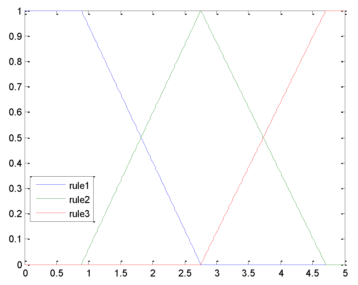
Rule 1: If x 2 ( k ) is small ( x 2 ( k ) is about 0.8862), then
x ( k + 1 ) = ( A 1 + Δ A 1 ) x ( k ) + ( A d 1 + Δ A d 1 ) x ( k d ( k ) ) + D 11 w ( k ) + G 1 f ( k ) ;
Rule 2: If x 2 ( k ) is medium ( x 2 ( k ) is about 2.7520), then
x ( k + 1 ) = ( A 2 + Δ A 2 ) x ( k ) + ( A d 2 + Δ A d 2 ) x ( k d ( k ) ) + D 12 w ( k ) + G 2 f ( k ) ;
Rule 3: If x 2 ( k ) is large ( x 2 ( k ) is about 4.7052), then
x ( k + 1 ) = ( A 3 + Δ A 3 ) x ( k ) + ( A d 3 + Δ A d 3 ) x ( k d ( k ) ) + D 13 w ( k ) + G 3 f ( k ) .
Here, x ( k ) and x ( k d ( k ) ) are the set of differences between the temperature state value and the corresponding equilibrium point temperature value. According to the selected parameters, there are
A 1 = [ 0 . 0418   0 . 0132 0 . 0346 - 0 . 0194 ] , A 2 = [ 0 . 0590 0 . 0346 - 0 . 0472 0 . 0515 ] , A 3 = [ 0 . 0498 - 0 . 0167 0 . 0983 0 . 0758 ] , A d 1 = A d 2 = A d 3 = diag { 0.25 , 0.25 } , F ( k ) = sin ( 0.6 k ) , C 2 = [ - 0.79 0.65 ] , H 1 = H 2 = H 3 = [ 0.2 0.01 ] , E a = [ 0 0.15 ] , E d = [ 0 0.2 ] , G 1 = [ 0.21 - 0.14 ] , C 3 = [ - 0.81 0.65 ] , G 2 = [ 0.20 - 0.12 ] , G 3 = [ 0.19 - 0.15 ] , D 21 = D 22 = D 23 = 0.02 , C 1 = [ - 0.8 0.65 ] .
The membership functions are shown in Figure 2.
The order of the fading model is = 2 , the probability quality function of the channel coefficient is as follows:
f ( β 0 ) = 0.0005 ( e 9.89 β 0 1 ) ,   0 β 0 1 f ( β 1 ) = { 10 β 1 , 0 β 1 0.20 2.50 ( β 1 1 ) , 0.20 < β 1 1 f ( β 2 ) = 8.5017 e 8.5 β 2 ,   0 β 2 1
The mathematical expectations β ¯ s ( s = 0 , 1 , 2 ) are acquired as 0.8991, 0.4000, and 0.1174, the variance ( β ˜ s ) 2 are 0.0133, 0.0467, and 0.01364, respectively. In terms of the above parameters and using the LMI toolbox in the Matlab software, the gains of the FD filter can be calculated by solving the feasible solution to matrix inequalities (23) and (24). The obtained gains of the fault detection filter (5) are shown in Table 1.
The initial state is taken as x ( 0 ) = [ 0.9 0.9 ] T , noise w ( k ) = { 0 . 2 rand ( 1 , 1 ) , 30 k 130 0 , else , and the fault signal f ( k ) is chosen as follows:
f ( k ) = { 1 , 50 k 100 0 , else
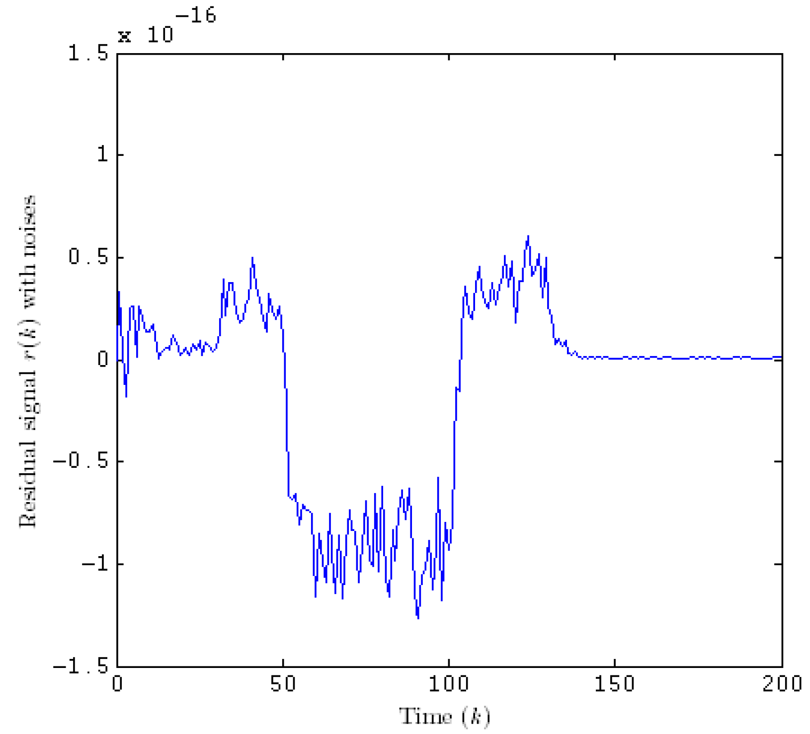
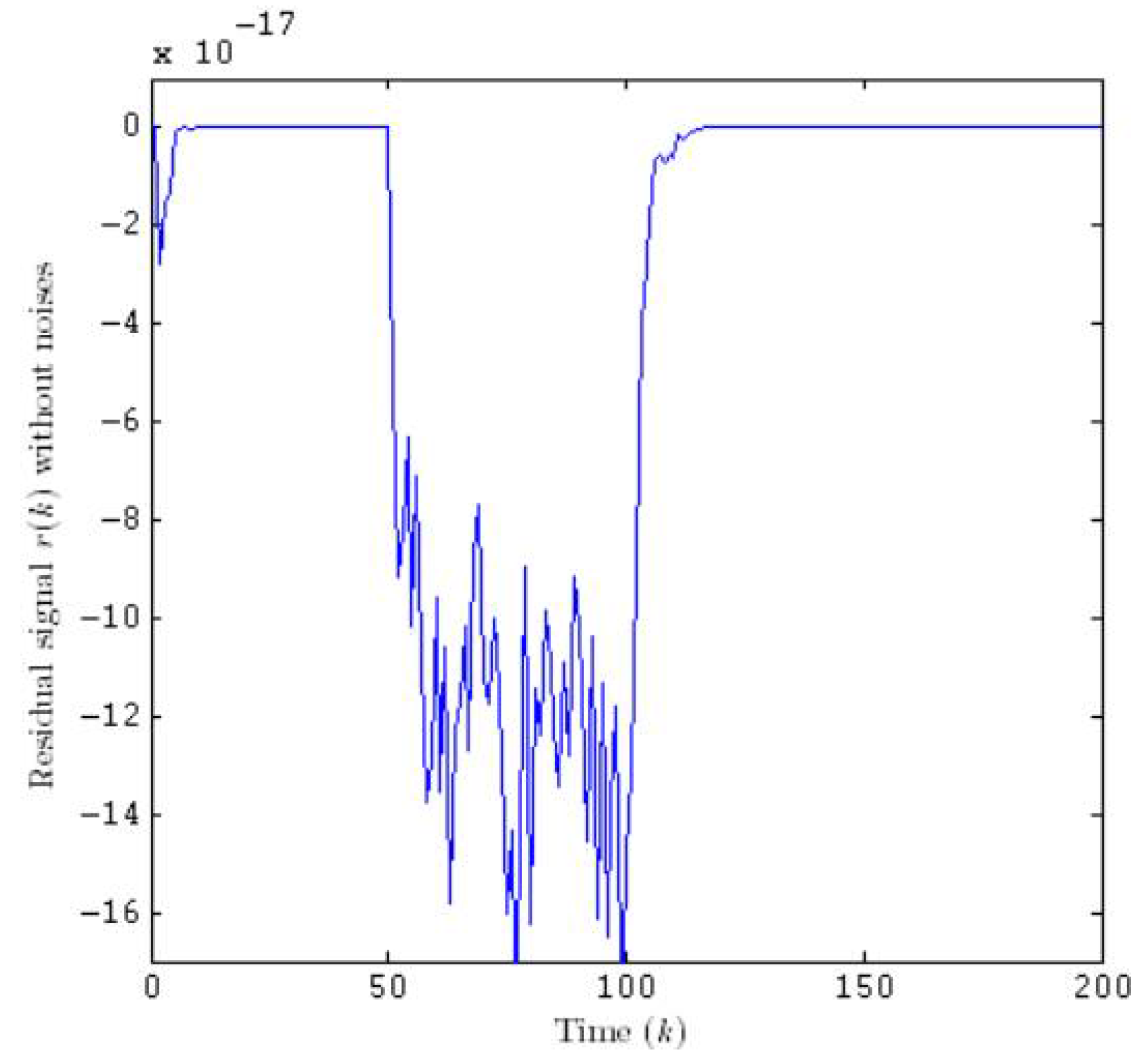
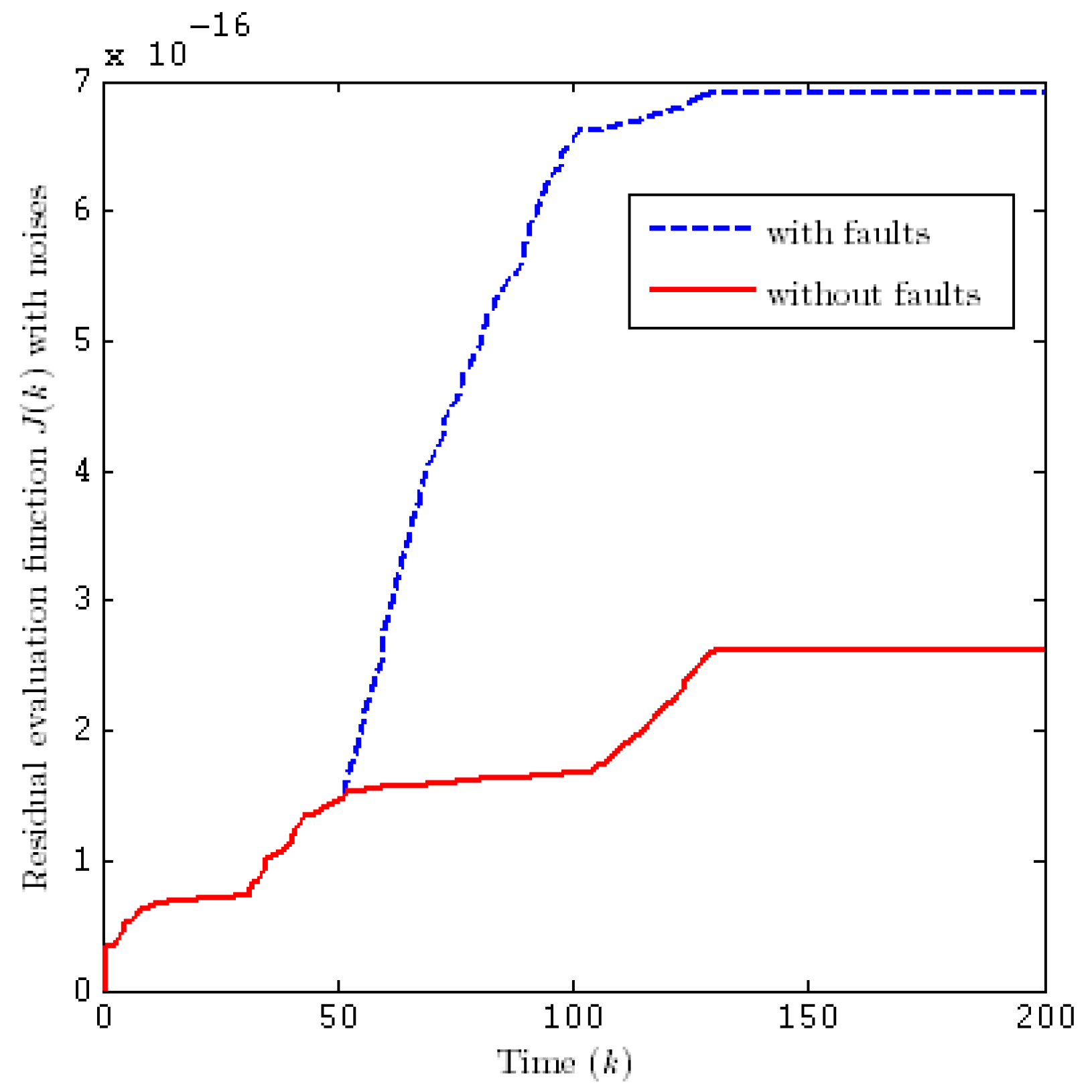
Figure 3 plots measurement curves, in which the dashed line denotes the ideal measurement output, and the solid line represents the signal actually received by the fault detection filter. It can be seen that the amplitude change of the received signal is more intense than that of the ideal measurement, which validates that channel fadings may lead to the signal distortion (signal missing and delays). Additionally, the occurrence and existence of faults cause the abnormal values of the measurement signals. Figure 4 and Figure 5 describe the residual signal curves with and without noise, respectively. We notice that the residual signal curve without noise is smoother than the one with noise, and the influence of both faults and channel fadings on the residual signal is obvious, which is in accordance with Equation (5). In terms of Equation (9), Figure 6 and Figure 7 reflect the evolution of the residual evaluation function curves with and without noise, respectively. It is shown that there are more fluctuations in the residual evaluation function with noise than those without noise. In Figure 6 (or Figure 7), the dashed line and the solid line depict the residual evaluation function with and without faults, respectively. It is also illustrated that the value of the residual evaluation function increases due to the existence of faults, which lay a basis for the fault detection.
Assuming the threshold J t h = sup f = 0 h = 0 200 r T ( h ) r ( h ) , after 200 fault-free simulation runs, the average threshold is then J t h = 0 . 2622 . It can be recognized from Figure 6 that 2.519 = J ( 59 ) < J t h < J ( 60 ) = 2.772 , i.e., the fault is detected in step 10, after it occurs. It can be concluded that the residual can not only reflect the fault in time, but also detect the fault in the case of disturbance.

6. Conclusions

In this paper, the FD issue for CSTR with respect to time delay, uncertainty parameters, and channel fadings was investigated in terms of the T-S fuzzy model. Norm-bounded uncertainties were adopted to describe parameter imprecision caused by modelling errors. The phenomenon of channel fadings was considered while the measurement output signal was transmitted from the sensor to the FD filter, which was then reflected with an improved L-th Rice fadings model. The performance constraints to be met by the constructed fault detection filter were both the exponential stability in the mean square of the filtering error system and the H disturbance rejection level of the residual filtering error in resistance to external disturbances. With the help of the Lyapunov stability theory and reinforced stochastic analysis techniques, the analysis of the performance and the design of the fault detection filter were carried out for the CSTR. As a result, a sufficient condition was put forward, ensuring the existence of a satisfactory FD filter. Simultaneously, a direct expression was acquired from the FD filter in accordance with the feasible solution to a specified LMI, which is solved conveniently via the standard Matlab software. Lastly, a simulation example demonstrated that faults can be reflected and detected in time under circumstances of disturbance by choosing the thresholds appropriately, which validates the effectiveness and the correctness of the developed FD strategy for CSTR in this paper. For subsequent research topics, we would like to deal with fault estimation, fault prognosis, and related issues therein [32].

Author Contributions

Model construction, system performance analysis, filter design, and writing—original draft preparation, Y.W.; investigation, D.Z.; writing—review and editing, Z.L.; supervision and project administration, W.R.; numerical simulation, J.L. All authors have read and agreed to the published version of the manuscript.

Funding

This research was funded by the Starting Fund for Doctoral Research of Daqing Normal University, grant number 19ZR09, and the Natural Science Foundation of Heilongjiang Province of China, grant number LH2021F006.

Institutional Review Board Statement

Not applicable.

Informed Consent Statement

Not applicable.

Data Availability Statement

Not applicable.

Conflicts of Interest

Authors declare no conflict of interest.

References

  1. Li, Y.; Feng, Y. T-S model based L2-L∞ control for continuous stirring tank reactor. J. Jilin Univer. (Inform. Sci. Ed.) 2014, 329, 247–253. [Google Scholar]
  2. Chen, Z.; Cao, Y.; Ding, S.X.; Zhang, T. A Distributed canonical correlation analysis-based fault detection method for plant-wide process monitoring. IEEE Trans. Ind. Inform. 2019, 15, 2710–2720. [Google Scholar] [CrossRef]
  3. Gao, Z.; Cecati, C.; Ding, S.X. A survey of fault diagnosis and fault-tolerant techniques—Part I: Fault diagnosis with model-based and signal-based approaches. IEEE Trans. Ind. Electron. 2015, 62, 3757–3767. [Google Scholar] [CrossRef] [Green Version]
  4. Gao, Z.; Cecati, C.; Ding, S.X. A survey of fault diagnosis and fault-tolerant techniques—Part II: Fault diagnosis with knowledge-based and hybrid/active approaches. IEEE Trans. Ind. Electron. 2015, 62, 3768–3774. [Google Scholar] [CrossRef] [Green Version]
  5. Gao, Z.; Sheng, S. Real-time monitoring, prognosis, and resilient control for wind turbine systems. Renew. Energy 2017, 116, 1–4. [Google Scholar] [CrossRef]
  6. Hou, N.; Wang, Z.; Ho, D.W.; Dong, H. Robust partial-nodes-based state estimation for complex networks under deception attacks. IEEE Trans. Cybern. 2020, 50, 2793–2802. [Google Scholar] [CrossRef]
  7. Chen, H.; Jiang, B.; Chen, W.; Yi, H. Data-driven detection and diagnosis of incipient faults in electrical drives of high-speed trains. IEEE Trans. Ind. Electron. 2019, 66, 4716–4725. [Google Scholar] [CrossRef]
  8. Gao, Z.; Liu, X. An Overview on Fault Diagnosis, Prognosis and resilient control for wind turbine systems. Processes 2021, 9, 300. [Google Scholar] [CrossRef]
  9. Ali, N.; Hong, J. Failure detection and prevention for cyber-physical systems using ontology-based knowledge base. Computers 2018, 7, 68. [Google Scholar] [CrossRef] [Green Version]
  10. Dong, H.; Hou, N.; Wang, Z. Fault estimation for complex networks with randomly varying topologies and stochastic inner couplings. Automatica 2020, 112, 108734. [Google Scholar] [CrossRef]
  11. Zhang, Z.; Yang, G. Distributed fault detection and isolation for multiagent systems: An interval observer approach. IEEE Trans. Syst. Man Cybern. Syst. 2020, 50, 2220–2230. [Google Scholar] [CrossRef]
  12. Ye, D.; Chen, M.; Yang, H. Distributed adaptive event-triggered fault-tolerant consensus of multiagent systems with general linear dynamics. IEEE Trans. Cybern. 2019, 49, 757–767. [Google Scholar] [CrossRef]
  13. Zhu, X.; Liu, Y.; Fang, J.; Zhong, M. Fault detection for a class of linear systems with integral measurements. Sci. China Inform. Sci. 2021, 64, 1–10. [Google Scholar] [CrossRef]
  14. Taoufik, A.; Defoort, M.; Djemai, M.; Busawon, K.; Sánchez-Torres, J.D. Distributed global actuator fault-detection scheme for a class of linear multi-agent systems with disturbances. IFAC-PapersOnLine 2020, 53, 4202–4207. [Google Scholar] [CrossRef]
  15. Alikhani, H.; Meskin, N. Event-triggered robust fault diagnosis and control of linear Roesser systems: A unified framework. Automatica 2021, 128, 109575. [Google Scholar] [CrossRef]
  16. Zhong, M.; Ding, S.X.; Zhou, D.; He, X. An Hi/ H∞ optimization approach to event-triggered fault detection for linear discrete time systems. IEEE Trans. Autom. Control 2020, 65, 4464–4471. [Google Scholar] [CrossRef]
  17. Ren, W.; Gao, M.; Kang, C. Non-fragile h-infinity fault detection for nonlinear systems with stochastic communication protocol and channel fadings. Int. J. Control Autom. Syst. 2021, 19, 2150–2162. [Google Scholar] [CrossRef]
  18. Ma, H.; Xu, L. Cooperative fault diagnosis for uncertain nonlinear multiagent systems based on adaptive distributed fuzzy estimators. IEEE Trans. Cybern. 2020, 50, 1739–1751. [Google Scholar] [CrossRef]
  19. Gao, Z. Estimation and compensation for Lipschitz nonlinear discrete-time systems subjected to unknown measurement delays. IEEE. Trans. Indust. Electron. 2015, 62, 5950–5961. [Google Scholar] [CrossRef]
  20. Liu, X.; Gao, Z.; Zhang, A. Observer-based fault estimation and tolerant control for stochastic Takagi–Sugeno fuzzy systems with Brownian parameter perturbations. Automatica 2019, 102, 137–149. [Google Scholar] [CrossRef]
  21. Ji, W.; Wang, T.; Qiu, J.; Fu, S. Distributed fuzzy H∞ filtering for nonlinear multi-rate networked double-layer industrial processes. IEEE Trans. Indust. Electron. 2017, 64, 5203–5211. [Google Scholar]
  22. Su, X.; Shi, P.; Wu, L.; Basin, M.V. Reliable filtering with strict dissipativity for T–S fuzzy time-delay systems. IEEE Trans. Cybern. 2017, 44, 2470–2483. [Google Scholar]
  23. Ali, M.S.; Gunasekaran, N.; Zhu, Q. State estimation of T–S fuzzy delayed neural networks with Markovian jumping parameters using sampled-data control. Fuzzy Sets Syst. 2017, 306, 87–104. [Google Scholar]
  24. Chibani, A.; Chadli, M.; Ding, S.X.; Braiek, N.B. Design of robust fuzzy fault detection filter for polynomial fuzzy systems with new finite frequency specifications. Automatica 2018, 93, 42–54. [Google Scholar] [CrossRef]
  25. Shen, Y.; Wang, Z.; Shen, B.; Fuad, E. Alsaadi. Event-based recursive filtering for a class of nonlinear stochastic parameter systems over fading channels. Int. J. Gen. Syst. 2018, 47, 401–415. [Google Scholar] [CrossRef]
  26. Zhang, Z.; Su, S.; Niu, Y. Dynamic event-triggered control for interval type-2 fuzzy systems under fading channel. IEEE Trans. Cybern. 2020, 99, 1–10. [Google Scholar] [CrossRef]
  27. Wang, Y.; Ren, W.; Lu, Y. Fault detection for complex systems with channel fadings, randomly occurring multiple delays and infinitely distributed delays. J. Syst. Sci. Complex. 2018, 31, 419–435. [Google Scholar] [CrossRef]
  28. Dong, H.; Wang, Z.; Lam, J.; Gao, H. Fuzzy-model-based robust fault detection with stochastic mixed time delays and successive packet dropouts. IEEE Trans. Syst. Man Cybern. Syst. 2012, 42, 365–376. [Google Scholar] [CrossRef] [Green Version]
  29. Li, M.; Yu, D.; Chen, Z.; XiaHou, K.; Ji, T.; Wu, Q.H. Data-driven residual-based method for fault diagnosis and isolation in wind turbines. IEEE Trans. Sustain. Energy 2019, 10, 895–904. [Google Scholar] [CrossRef]
  30. Guan, X.P.; Chen, C.L. Delay-dependent guaranteed cost control for T-S fuzzy systems with time delays. IEEE Trans. Fuzzy Syst. 2004, 12, 236–249. [Google Scholar] [CrossRef]
  31. Wang, Z.; Ho, D.; Liu, Y.; Liu, X. Robust H∞ control for a class of nonlinear discrete time-delay stochastic systems with missing measurements. Automatica 2009, 45, 684–691. [Google Scholar] [CrossRef] [Green Version]
  32. Djeziri, M.; Nguyen, T.-B.-L.; Benmoussa, S.; M’Sirdi, N. Fault prognosis based on physical and stochastic models. In Proceedings of the 2016 European Control Conference, Aalborg, Denmark, 29 June–1 July 2016; pp. 2269–2274. [Google Scholar]
Figure 1. Schematic of CSTR.
Processes 09 02127 g001
Figure 2. Membership function.
Processes 09 02127 g002
Figure 3. Ideal and practical measurement outputs.
Processes 09 02127 g003
Figure 4. Residual signal with noise.
Processes 09 02127 g004
Figure 5. Residual signal without noise.
Processes 09 02127 g005
Figure 6. Residual evaluation function with noise.
Processes 09 02127 g006
Figure 7. Residual evaluation function without noise.
Processes 09 02127 g007
Table 1. The computed gains of the fault detection filter.
A f i B f i C f i D f i
i = 1 [ 0.8972 0.7112 0.4820 0.4996 ] [ 0.0145 0.0017 ] [ 0.0893 0.4515 ] 2.4358
i = 2 [ 0.4122 0.3698 0.6324 0.5753 ] [ 0.0166 0.0139 ] [ 0.4414 0.3681 ] 5.2732
i = 3 [ 0.0014 0.0012 0.0002 0.0002 ] [ 0.0489 0.0214 ] [ 0.1356 0.0628 ] 7.4592
Publisher’s Note: MDPI stays neutral with regard to jurisdictional claims in published maps and institutional affiliations.