Article

Optimisation of a Side Inlet for H2 Entry into an Ultrasonic Spray Pyrolysis Device

Faculty of Mechanical Engineering, University of Maribor, Smetanova ulica 17, 2000 Maribor, Slovenia
*
Author to whom correspondence should be addressed.
Processes 2021, 9(12), 2256; https://doi.org/10.3390/pr9122256
Submission received: 29 October 2021 / Revised: 9 December 2021 / Accepted: 10 December 2021 / Published: 14 December 2021
(This article belongs to the Topic Modern Technologies and Manufacturing Systems)

Abstract

:
An ultrasonic spray pyrolysis (USP) device consists of an evaporation and two reaction zones of equal length, into which an aerosol with a precursor compound enters, and where nanoparticles are formed in the final stage. As part of this research, we simulated the geometry of a side inlet, where the reaction gas (H2) enters into the reaction tube of the device by using numerical methods. Mixing with the carrier gas (N2) occurs at the entry of the H2. In the initial part, we performed a theoretical calculation with a numerical simulation using ANSYS CFX, while the geometries of the basic and studied models were prepared with Solidworks. The inlet geometry of the H2 included a study of the position and radius of the inlet with respect to the reaction tube of the USP device, as well as a study of the angle and diameter of the inlet. In the simulation, we chose the typical flows of both gases (N2, H2) in the range of 5 L/min to 15 L/min. The results show that the best geometry is with the H2 side inlet at the bottom, which the existing USP device does not allow for. Subsequently, temperature was included in the numerical simulation of the basic geometry with selected gas flows; 150 °C was considered in the evaporation zone and 400 °C was considered in the other two zones—as is the case for Au nanoparticle synthesis. In the final part, we performed an experiment on a USP device by selecting for the input parameters those that, theoretically, were the most appropriate—a constant flow of H2 5 L/min and three different N2 flows (5 L/min, 10 L/min, and 15 L/min). The results of this study show that numerical simulations are a suitable tool for studying the H2 flow in a UPS device, as the obtained results are comparable to the results of experimental tests that showed that an increased flow of N2 can prevent the backflow of H2 effectively, and that a redesign of the inlet geometry is needed to ensure proper mixing. Thus, numerical simulations using the ANSYS CFX package can be used to evaluate the optimal geometry for an H2 side inlet properly, so as to reconstruct the current and improve future USP devices.

Graphical Abstract

1. Introduction

Nanoparticles range in size from 0.1 nm to 100 nm, and gold nanoparticles have recently been at the forefront of research. This is due to their different properties [1] compared to bulk gold, which are known at the macro level. Gold nanoparticles have a large surface area in terms of volume, so they are useful for many new applications. They have functional properties, among which biocompatibility and catalytic activity make them different from other metal nanoparticles [2,3].
Ultrasonic spray pyrolysis (USP) is a method of nanoparticle synthesis. Compared to other methods (laser ablation [4], nanoemulsion [5], reduction in liquid [3]) it enables the continuous synthesis of nanoparticles and represents a promising method for their industrial production [6]. The existing USP device (Figure 1) [7], which has three temperature zones, allows for the controlled synthesis of metal nanoparticles on a laboratory scale. They are synthesised by the transformation of the pre-prepared solution (the so-called precursor) by ultrasound into an aerosol, which is transported with the help of a carrier gas within three zones of the heated reaction tube. In the first zone, the solvent evaporates. In the second, the thermal decomposition of the precursor compound and the reaction with H2 gas occur, and the nanoparticles are densified in the third zone. Thus, the formed nanoparticles can be trapped in liquid, where a suitable stabiliser is dissolved, which prevents their possible agglomeration [1].
The H2 gas enters a USP device in the second zone via a side inlet at a fixed inlet angle with respect to the reaction tube. The inlet angle and geometry must be chosen to ensure the proper mixing of the carrier gas, reaction gas, and precursor compound, with the aim of producing as many controlled nanoparticles as possible, defined by the target final size and shape. Effective mixing of all the components is key to ensuring a fast and reliable synthesis. Common issues that can be attributed to bad mixing include unreacted residue, which can exacerbate the agglomeration of the suspended nanoparticles, and material losses due to the backflow of reduction gas into the evaporation chamber, causing the premature formation of nanoparticles that are deposited on the walls of the reaction tube.
The numerical models used by Wang [8] and Ternik [9] have been shown to be able to simulate the behaviour of aerosolised droplets in a USP device effectively. Therefore, computer fluid dynamics (CFD) seemed to be an appropriate path for the purpose of evaluating the most optimal geometry and dimensions of the side inlet for H2 gas into a three-zone USP device. To achieve this, we used a (CFD) programme, which is, nowadays, an essential tool for fluid dynamics.
With the ANSYS CFX programme, we can model and prepare geometries for simulations, and the programme also supports various types of files from other modelling programmes [10]. All computer fluid dynamics programmes follow basic conservation laws. As part of our scientific work, we performed the law of conservation of mass, the law of conservation of momentum, and the law of conservation of energy when performing all simulations. Detailed records of all laws are presented in references [11,12]. The “thermal energy” model was used to calculate the heat transfer. The Reynolds-averaged Navier–Stokes (RANS) approach was used for modelling the turbulent flow, with which one-equation and two-equation turbulent models can be used to calculate fluctuating current field quantities. In the presented research work, we used a two-equation k–ε turbulent model to inventory the turbulent flow [13].
As industrial applications of USP are still relatively rare [14,15], significant optimisation steps must be taken in order to improve the method’s viability and efficiency within an industrial setting [16]. In order to obtain sustainable mixing and prevent the agglomeration of nanoparticles, which is common in the current design of the USP device, the optimisation of the reaction gas inlet was performed in the presented study. The obtained results indicate that the proper design of the reaction gas inlet can eliminate backflow (leakage). This results in the production of nanoparticles with different sizes and characteristics for a broader range of operating regimes, and it brings the usability of USP devices closer to the industrial scale. The presented study also indicates that numerical simulations are an appropriate tool for studying flow in a USP device. The obtained results give significant information about gas flow in the device and enable the study of possible future designs of USP devices.

2. Materials and Methods
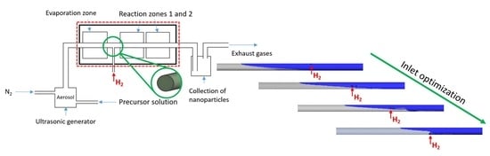
2.1. USP Device

The USP device is shown schematically in Figure 1. The ultrasonic generator has a diameter of 20 mm, operates at a frequency of 1.6 MHz, produces aerosol droplets of 3 µm, and is able to convert 500 mL/h of liquid into an aerosol [7]. The furnace has a metal housing and fireclay brick insulation inside. Rock wool is used around the reaction tube so that it does not rest on the brick, and the insulation is tight. The furnace has a temperature regulator on the side for each zone separately. All glass tubes in the UPS device are made of quartz glass [17,18].
The USP device has 3 zones. The first is an evaporation zone in which the solvent evaporates, and it operates at temperatures of 100 to 300 °C. The second is the reaction zone into which the H2 [19,20,21,22,23,24], enters and where the reaction with the precursor compound takes place. It has temperatures from 400 °C to 1000 °C. The last zone can be a reaction or cooling zone, so temperatures range from 20 °C to 1000 °C. Temperature setting and monitoring were performed with a temperature controller located directly on the furnace (Pixsys, model ATR244). N2 was used as the carrier gas [19,21,25,26]. Gas flow control instruments were from the manufacturer Messer, with a maximum flow of 16 L/min or a minimum flow of 1 L/min at 1 bar, and with a possible step-scale of 1 L/min.
The photo in the process of the experiment was taken with a Nikon D7500 camera and a Nikkor AF-S f2.8 24–70 mm lens.
In the case of the presented research, where the optimisation of the H2 side inlet was performed, we had to consider the following limitations and assumptions: (i) experimental testing was performed on the basic geometry of the USP device; (ii) the research work focused only on the flow in the reaction tube, and not on the entire USP device; (iii) the experimental testing was performed with coloured water vapour (green pigment), which was not taken into account in the simulations; (iv) the numerical simulation was performed on at least three different geometries; and (v) nanoparticles were not considered in the simulations and experimental testing.

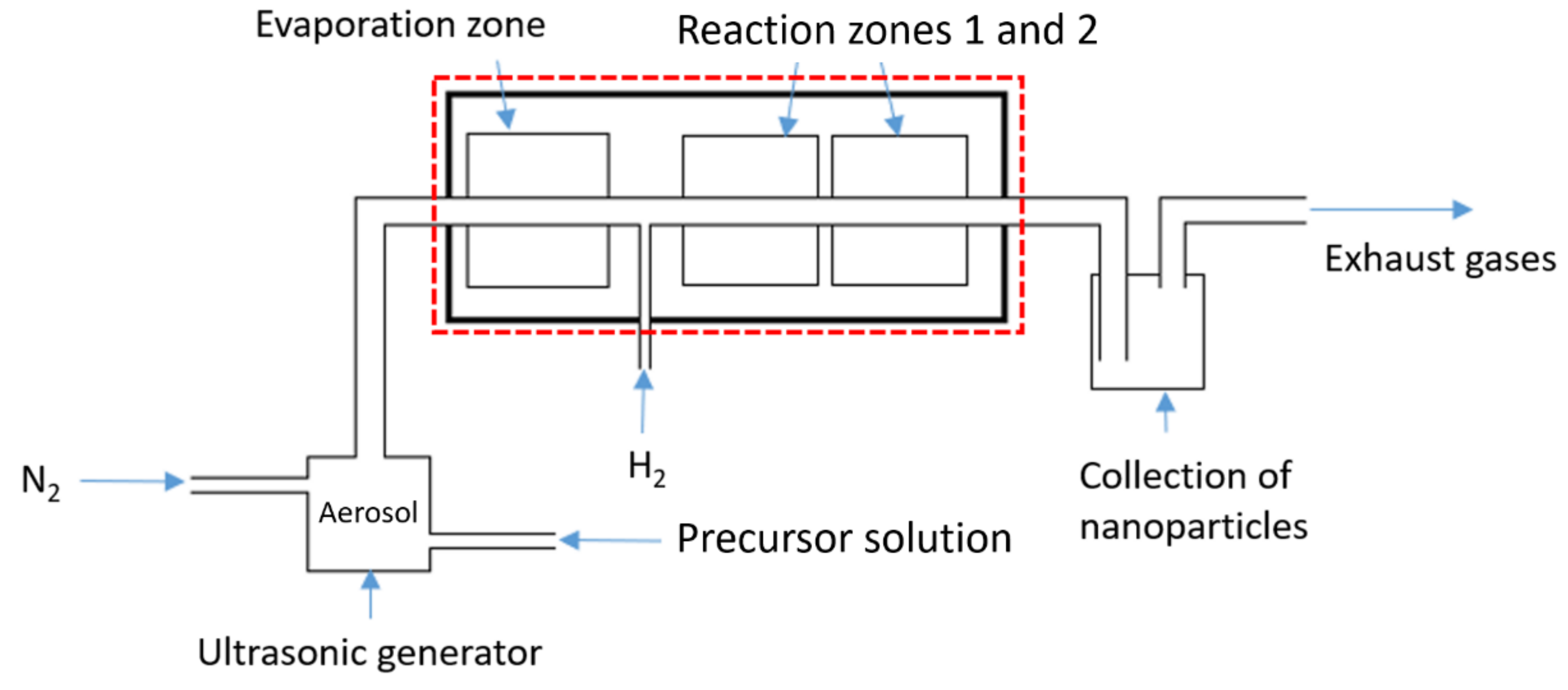
2.2. Numerical Model—Description of the Geometry

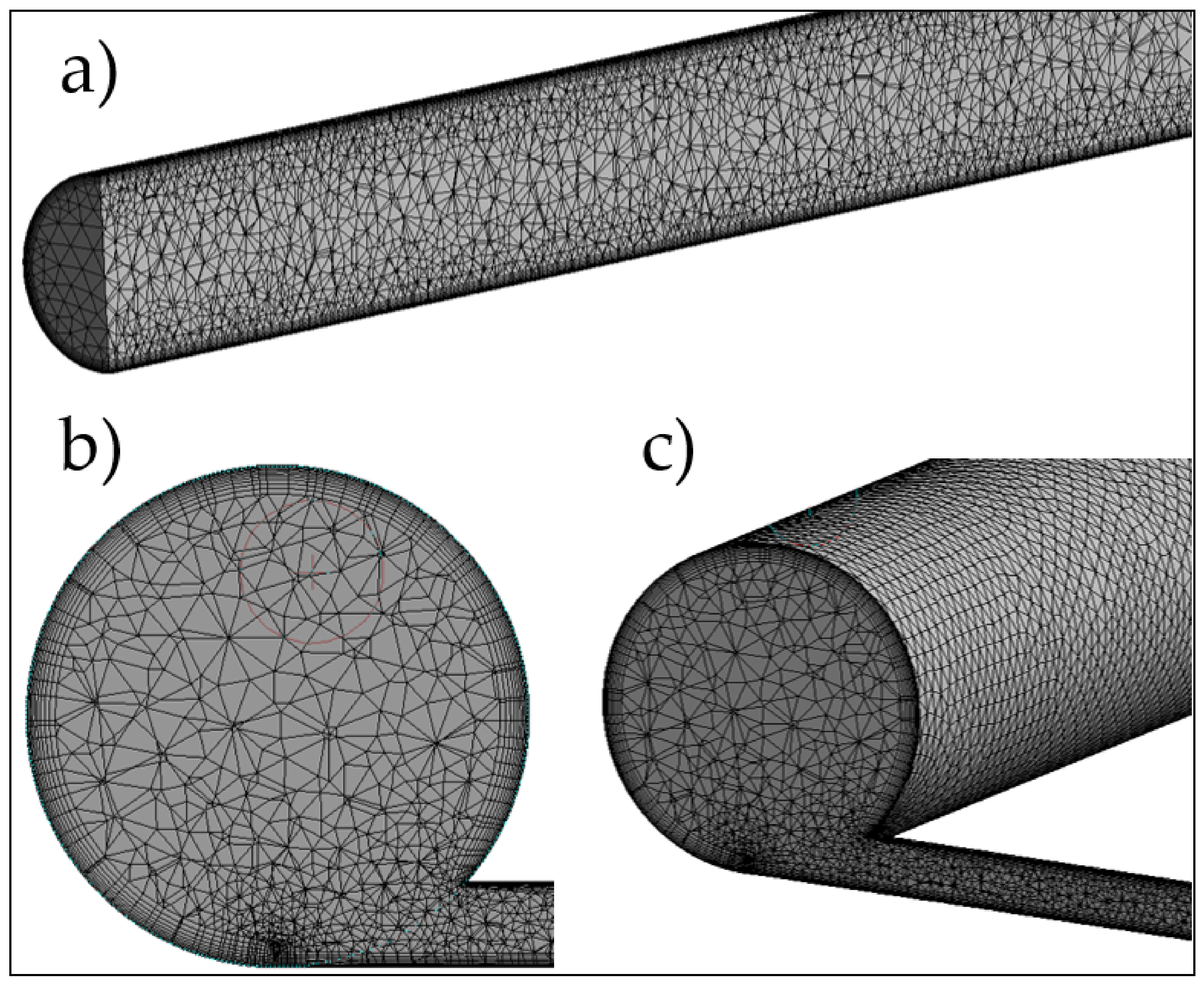
2.2.1. Description of the Geometry

All geometries were formed from a reaction tube, with a length of 1780 mm, an inner diameter of 35 mm, and an outer diameter of 40 mm, and a side inlet, which has a centreline at 655 mm from the entrance of the reaction tube due to the shape of the furnace of the USP device. The side inlet has an inner diameter of 6 mm and an outer diameter of 10 mm. In the basic geometry, the side inlet enters the main tube at an angle of 90° to the reaction tube, as shown in Figure 2.

2.2.2. New Geometries—A Case Study

As part of the research, we prepared new side-feed geometries, which are shown in Table 1. The following references [27,28,29,30,31] were helpful in selecting the different geometries. The geometries differed in the inlet angle of the side inlet for H2. The side inlet had an inside diameter of 6 mm in all cases except for the last geometry, where we considered an inside diameter of 10 mm.
For the mesh of the basic model we chose CFD for “physics preference”, CFX for “solver preference”, and 10 mm for the size of the elements. The reaction tube and side feed were then crosslinked separately. For the reaction tube (Figure 3a), the size of the mesh elements was chosen to be 2.5 mm, and an “inflation layer” was added, which is a layer on the tube walls that makes the mesh denser and allows for a more accurate calculation of the boundary layer. This layer had a thickness of 2 mm and was distributed across 10 layers of elements. Based on the thickness and the growth factor, which was 1.2, the programme itself determined the thickness of the layers. For the side inlet (Figure 3b,c), we selected the size of the grid elements as 1 mm, to which we also added the “inflation layer”. This layer had a thickness of 1 mm, 8 layers, and a layer growth factor of 1.2.
With this method, we got a computational mesh with 1.24 million elements. The references [32,33,34] were helpful when preparing the computational mesh. The same settings were used in the preparation of the computational meshes of all the new geometries.

2.3. Conditions

To determine the H2 flow, it was necessary to make certain calculations, which showed that the theoretical minimum required flow was 3.3 L/min. Therefore, a minimum flow rate of 5 L/min was chosen for the study. A gas temperature of 20 °C was used for the simulations. The gravitational force (9.81 m/s2) was considered in the simulations. It was necessary to determine the inlet, outlet, and walls on the numerical model. The inlet to the reaction tube to which N2 was fed is marked as “IN1”, the inlet to the side feed to which H2 was fed is marked as “IN2”, and the outlet from the reaction tube is “OUT” (Figure 4).

2.3.1. Conditions for Basic Geometry Disregarding Temperature

For the basic geometry, we decided to perform simulations at five different boundary conditions. We chose different combinations of H2 and N2 flows. With the selected combinations, we wanted to gain theoretical insight into the events in the evaporation and reaction zones of the considered UPS device, and, thus, indirectly, the influence of the flow of an individual gas on the events in the USP process. The selected flows are shown in Table 2.

2.3.2. Conditions for Basic Geometry Taking into Account Temperature

Subsequently, we also performed a simulation on the basic geometry considering the temperatures in all three zones of the furnace. The first zone is the evaporation zone, for which a temperature of 150 °C was selected, the second is the reaction zone, in which the temperature was 400 °C, and the third, the reaction or cooling zone, also had a temperature of 400 °C. For the flow boundary conditions, we used the flows of the third simulation of the basic geometry, with a flow rate of H2 5 L/min and N2 10 L/min, as it was necessary to ensure a sufficient flow rate of N2 for the reaction to take place in the reaction zones. In the temperature-based simulations, we had to adjust for the carrier and reaction gases that the density of the gases varied with the temperature. We did this by writing the equations in the CEL module of the CFX programme. We also marked the points on the model where we monitored the gas temperatures (Figure 5). These points included Point 1—beginning of the evaporation zone; Point 2—end of the evaporation zone; Point 3—end of the first reaction zone; Point 4—end of the second reaction zone.

2.3.3. New Geometries

For all new geometries, we had a flow of both gases of 5 L/min, as we wanted to determine a geometry in which H2 would not leak back through the tube, even at the lowest flows. Simulations for all geometries were performed without considering the wall temperatures.

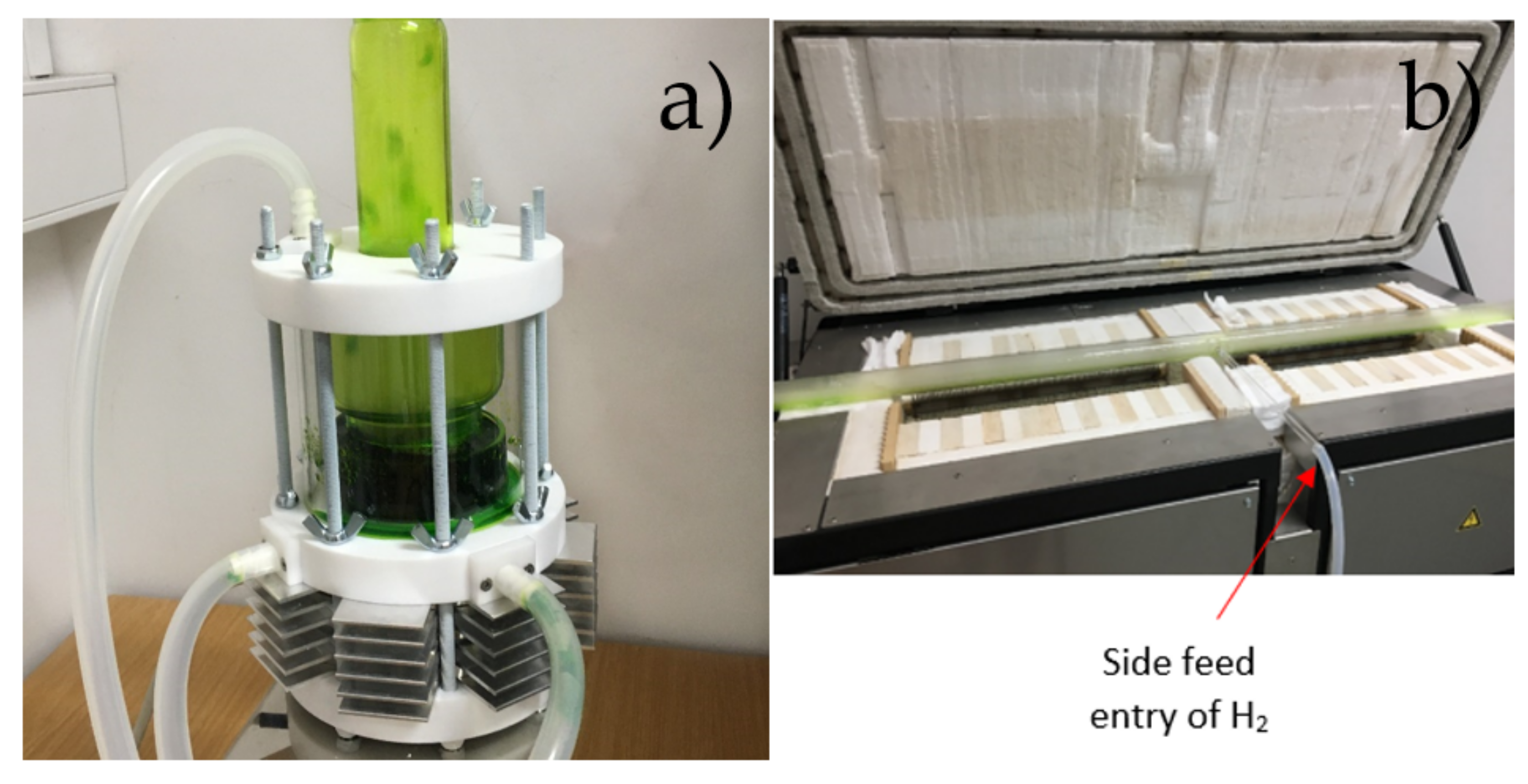
2.4. Experimental Setup

The experimental test in the USP device was performed by staining the water with a water-soluble organic dye powder of green colour (E142). When the ultrasonic generator was started, an aerosol was formed from the water, which was transported to the reaction tube with the help of N2, and H2 was fed to the side inlet. The reaction tube was eventually opened without a collection system because we did not produce nanoparticles that would need to be collected. The experiments were performed at three different N2 flows and a constant H2 flow, as shown in Table 3. The flows were selected based on those used later in the simulations.
To facilitate the monitoring of the aerosol transport process in the USP device reaction tube and to observe the mixing of N2 and H2, the experiment was performed by lifting the device cover as well as the quartz tube. For better visibility, we used an additional light source (a lamp) to be able to capture the key moments of the mixing of all the components (gases and aerosol) in the reaction tube with the camera. The results of the experimental testing were used further for the validation of the numerical results on the basic geometry.

3. Results

3.1. Results of the Numerical Simulations

All simulations were performed as time dependent. The total time of each simulation was 10 s. The selected time step was Δt = 0.01 s. We set the value of 10–4 s for the convergence criterion. The average time of one simulation was 8 h. The presented results show the conditions at 10 s of flow in the model. In all presentations of the results, the H2 profile is coloured blue and the N2 profile is grey.

3.1.1. Results of Simulations on the Basic Geometry

First, simulations were performed with different flows on the basic geometry. All the results shown in Table 4, show the state in the reaction tube after 10 s of current.
We found that in the simulations of the basic geometry, the N2 flow had the greatest influence on the H2 leakage back into the reaction tube. The leakage profile H2 is wedge-shaped. The calculations show that at a flow of N2 and H2 5 L/min, the wedge length was approximately 250 mm. At flows of N2 = 5 L/min and H2 = 10 L/min, it was approximately 300 mm, and at flows of N2 = 10 L/min and H2 = 5 L/min, it was approximately 25 mm. For other flows, the leakage was negligible, or no H2 leakage was obtained.

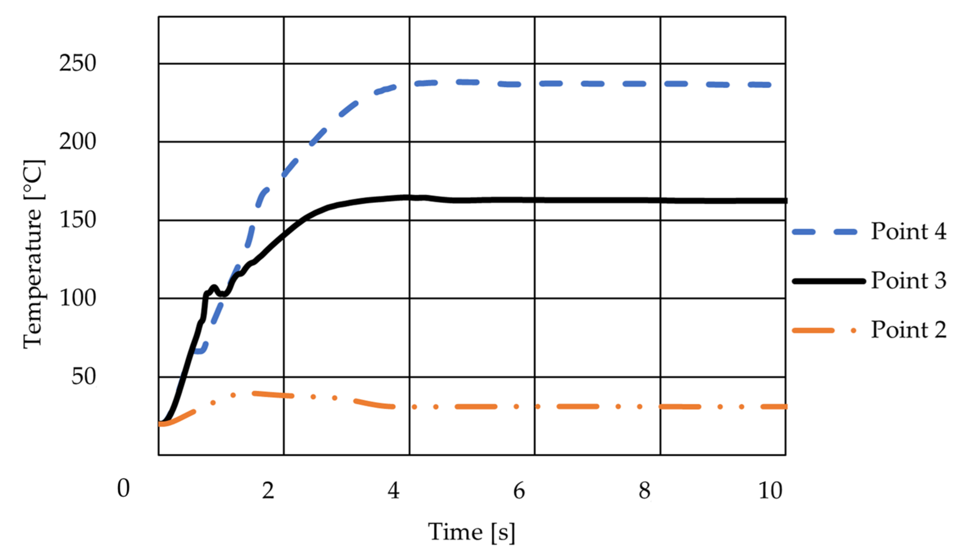
3.1.2. The Results of the Simulation of the Basic Geometry with Regard to Temperature

For the temperature-based simulation, flow rates of H2 = 5 L/min and N2 = 10 L/min were selected. These flows were chosen because they proved to be the most optimal if we did not consider other external conditions. The inlet temperature of the gases was 20 °C. The graphical results of the numerical simulation are shown in Figure 6.
Prior to the simulation, we marked the points on the model at which we measured the gas temperatures (5). At Point 1, the constant temperature was 20 °C. The highest calculated simulation temperatures at the other points were as follows: Point 2—39.8 °C, Point 3—164.6 °C, Point 4—238.4 °C. In this simulation, it was shown that H2 was not leaking back, but sufficient temperatures were not reached (Figure 7).

3.1.3. Results of Simulations on the New Geometries

The results of simulations on the new geometries are shown in Table 5. Of all the selected different geometries, geometry No. 2, where the side feed was at the bottom of the reaction tube, the backflow of H2 was the lowest. For other geometries, H2 leaked back down the reaction tube to at least one-third of its length, its leakage profile being wedge-shaped. For this purpose, we also performed a simulation considering the temperature on geometry No. 2.

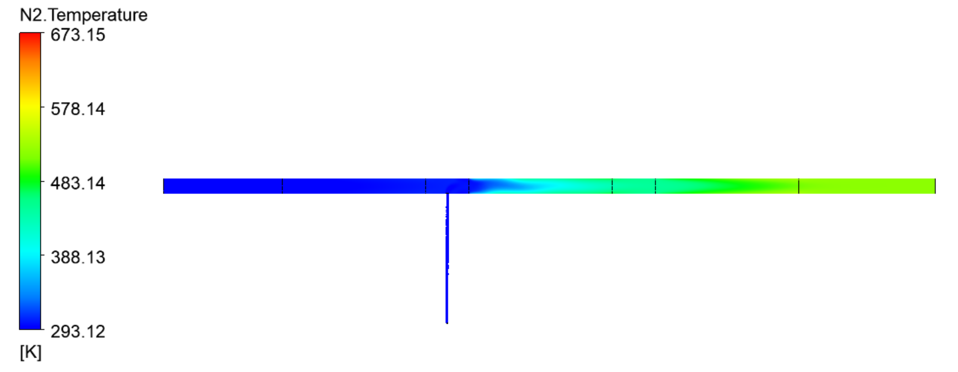
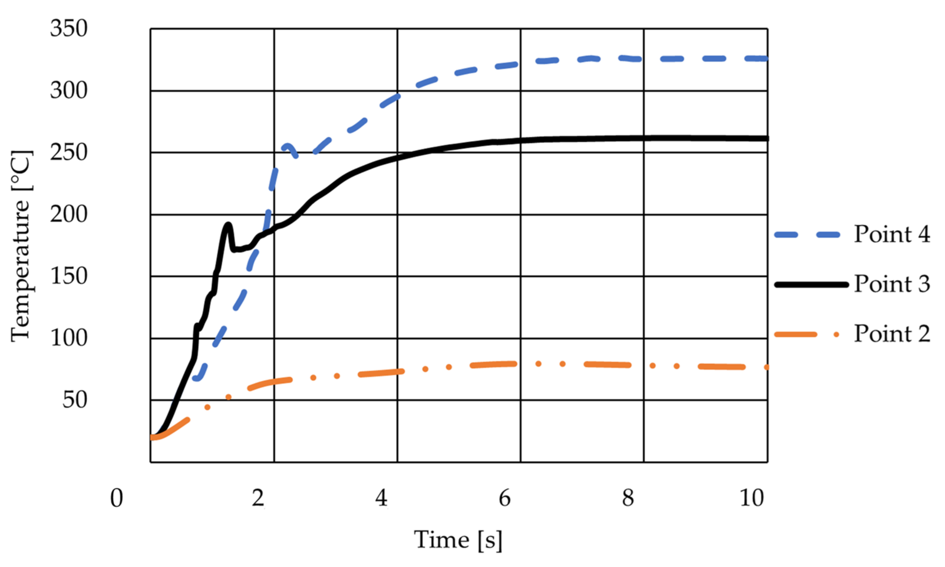
3.1.4. Temperature-Based Simulation on Geometry No. 2 by Entering the Side Inlet at the Bottom of the Reaction Tube

For the simulation of the new geometry, taking into account the temperature, we determined that the flow of both gases was 5 L/min, the temperature of the evaporation zone was 150 °C, and the temperature of both reaction zones was 400 °C. The inlet temperature of the gases was 20 °C. The simulation shown in Figure 8 shows that H2 would still leak back, but much less so than in the basic geometry simulation with the same flows.
Figure 9 shows how H2 cooled N2 at the entrance to the reaction tube since the N2 had a higher temperature when leaving the evaporation zone than when entering the first reaction zone.
The temperature measurement points during the simulation were the same as in the simulation with the basic geometry (Figure 5). The calculated simulation temperatures at the points were as follows: Point 2—79.5 °C, Point 3—261.9 °C, Point 4—326.5 °C. The differences in the calculated temperatures between the basic and the new geometries were due to the lower N2 flow. The calculations also show that the temperatures stabilised later than in the basic geometry simulation (Figure 10). The results of our simulations were also compared with other studies [34,35,36,37,38,39,40,41,42] and were consistent.

3.2. Results of Experimental Tests

During the experiment, it was observed that the ultrasonic generator generated a sufficiently large amount of aerosol, which the N2 transported successfully to the evaporation zone of the reaction tube. During this aerosol transport, the pigment was deposited on the walls of the reaction tube of the USP device, as shown in Figure 11.
Accurate observations and monitoring of the process show that before the side inlet, that is, before the entry of H2, the flow of aerosol and carrier gas was laminar (Figure 12). In the part of the side feed where the H2 entered, it was possible to see how it entered, the collision of the H2 molecules with the wall of the reaction tube, and the process of displacing the H2 with N2 molecules, which are generally 14× heavier than H2. From this point on, before the first reaction zone, it was seen that the flow of the mixture of both gases and vapour was turbulent (Figure 12). Based on the obtained images, we determined that the turbulent flow zone started at 15 mm from the side inlet, centrally in front of the first reaction zone (Figure 12). At the maximum N2 flow rate (15 L/min), the experiment did not show that H2 would leak back into the evaporation zone, as shown in Figure 13.
In the experiment, when the N2 and H2 flows were 5 L/min, it was possible to observe the leakage of H2 back into the evaporation zone (Figure 14). The leakage profile is wedge-shaped, with a measured length of 155 mm into the evaporation zone. The Video S1: H2—backflow is available online.
Among the results of the performed simulations and experiments, the following consistencies were confirmed. Changes in the flow at the entry of the H2 were laminar to turbulent. H2 displaced N2 at lower flows in the upper part of the reaction tube, causing H2 leakage back into the evaporation zone. The H2 leakage profile into the evaporation zone was wedge-shaped; with the numerical simulation, the length of the H2 leakage wedge was calculated to be approximately 250 mm, while the experiment showed a wedge length of approximately 155 mm. The reasons for the deviation in length are more than an incomplete consideration of the actual situation and include other restrictions, such as the accuracy of the gas flow regulators, and so forth. A high N2 flow (>10 L/min) prevented H2 leakage back into the evaporation zone, which reduced the process of displacing H2 with N2.
The general conclusion of the comparison of the results is that the numerical simulations predicted a longer wedge range, where the return flow (leakage) of H2 occurred. Thus, the results were not quantitatively comparable to the experimental tests. However, numerical simulations can predict the trend of H2 behaviour of the flow in the reaction tube, so they can be used to study the process of optimising the design of individual elements of the USP device.

4. Discussion

Limitations and understanding of the USP process were the basis for conducting a theoretical study with numerical methods. We first performed simulations with minimum and maximum flow values (H2 flow of 5–10 L/min and N2 flow of 5–15 L/min) so that we could gain insight into the processes and events in the selected zones. The research work was related to limitations, among which the key one was not allowing for the change of the basic geometry of the USP device, which has constrained reaction tube dimensions—length = 1780 mm, inner ϕ = 35 mm, and outer ϕ = 40 mm; the side feed is located at 655 mm from the entrance of the reaction tube and has an inner ϕ of 6 mm and an outer ϕ of 10 mm. In this way, we obtained information for the possible optimisation of the structural parts of the USP device in the future. Despite the above limitation, it was possible to change the gas flows in the existing USP device, as enabled by the flow regulator for H2 or N2. As it is difficult to regulate and measure the gas flows precisely, they were chosen so that they would not deviate too much and, thus, influence the course of the experiment (5, 10, 15 L/min). On the USP device, it was also possible to change the temperatures of individual zones. During the setting, the selected operating temperature rose evenly in all three zones. The experiment was performed by first mixing the pigment in deionised water, following the references of other authors [43], stating that the aerosol retains colour. The USP system was operated by pumping coloured water from a reservoir that was filled to the top before start-up into an ultrasonic generator. This was followed by the activation of the ultrasonic generator and, immediately afterwards, the opening of the N2 carrier gas supply valve, which transported the aerosol into the reaction tube. During the transport process, aerosol droplets in the carrier gas stream were deposited on the walls of the feed tube (before entering the reaction pipe, where they condensed and collected on the inner wall of the tube). This was followed by the opening of the valve on the side inlet, allowing H2 to enter the reaction tube. During this process, the formation of a wedge-shaped H2 profile was observed, which did not separate the boundary sharply from the rest of the mixture (Figure 14). Before entering the heating part of the reaction tube, aerosol retention was observed at the bottom of the tube, which was seen by the fact that there was greater transparency in the upper half of the reaction tube than in the lower half (Figure 14). This suggests that the mixed pigment increased the density of the aerosol, which was higher than the density of the N2. Based on the perceived effect of raising the carrier gas above the aerosol, it is necessary to point out that when preparing the precursor solution and the formation of the aerosol, it is necessary to know the density of the formed droplets. In this way, a suitable inert carrier gas can be selected, which must be denser than the aerosol to ensure a sufficient flow of the precursor compound to the reaction part of the USP device where the nanoparticles are formed. When monitoring the experiment, we could not provide the optimal viewing angle due to the placement of the USP device, so the images are not the best in terms of resolution. For further research and to achieve better resolution on the USP process monitoring images, it would be necessary to provide a more appropriate background and illumination of the reaction tube to obtain an even more accurate H2 wedge profile. We found that the wedge formed by the displacement of H2 was technologically problematic, as H2 escaping through the tube back into the evaporation zone can cause too rapid a reaction with the precursor compound at a lower temperature, leading to irregular nanostructures with inadequate chemical composition. Such nanoparticles are unusable for many intended applications, as they do not achieve the required properties related to their size and structure [3,4,5,6,7].

5. Conclusions

The study came to the following scientific conclusions:
  • The results of numerical simulations, in which the H2 inlets above and below were compared, show that placing the inlet on the bottom is the best proposed design solution for the USP device.
  • H2, which entered from the side inlet into the reaction tube of the USP device, escaped back into the evaporation zone because N2 displaced it at lower flows (5 L/min). The leakage profile H2 was wedge-shaped.
  • To prevent H2 leakage back into the evaporation zone, it was necessary to increase the N2 carrier gas flow to at least 10 L/min.
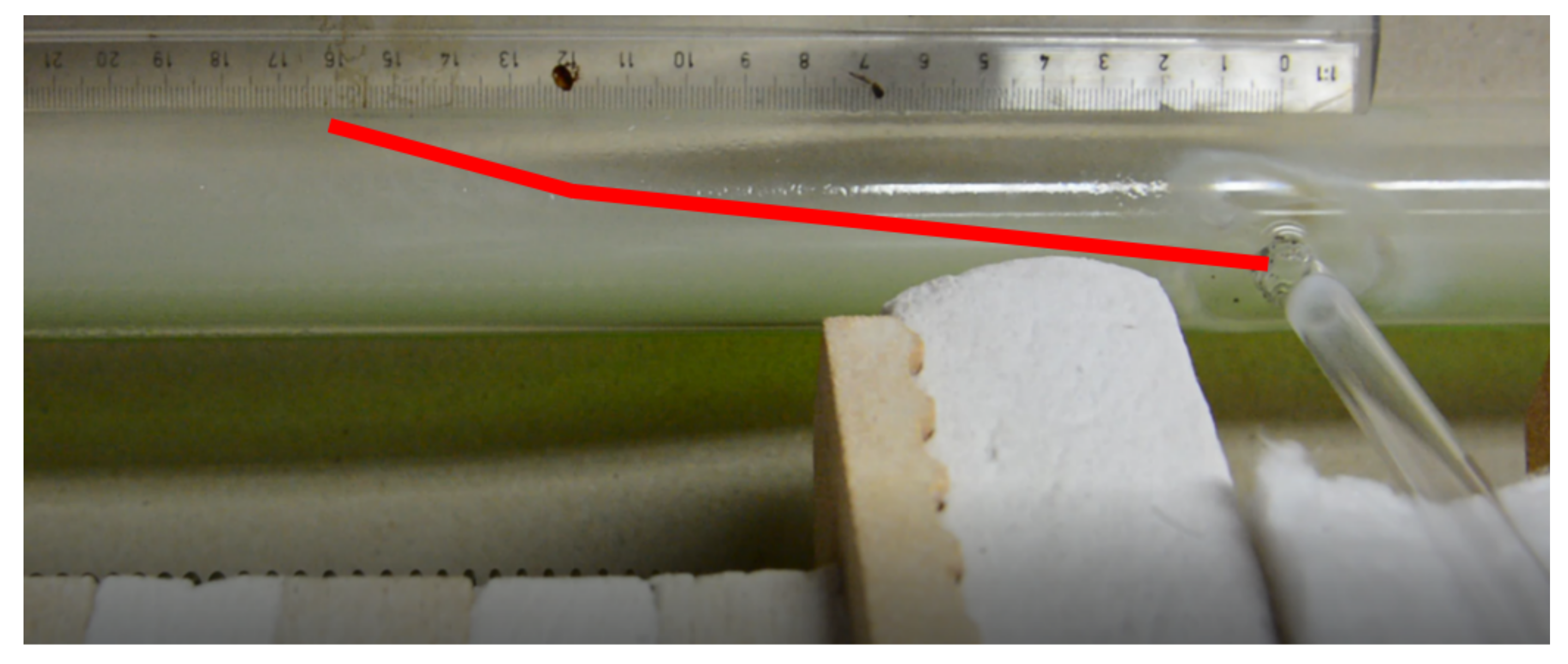
  • The experiment showed that the turbulence zone occurred approximately 15 mm from the side inlet in the reaction tube after H2 entered at a flow rate of 5 L/min and a N2 flow rate of 10 L/min.
  • Due to the high flow of N2, cooling occurred in the reaction tube of the USP device, so it was necessary to ensure higher temperatures in all three zones of the USP device with temperature control, or to extend the lengths of the zones in the USP device.
  • The results of the validation with the experiment showed that the numerical simulations give results with reasonable accuracy and are able to predict the flow in the glass tube of the USP device qualitatively. The numerical approach provides results with sufficient accuracy and can provide trends for the future optimisation of USP devices.

Supplementary Materials

The following is available online at https://www.mdpi.com/article/10.3390/pr9122256/s1, Video S1: H2—backflow.

Author Contributions

Conceptualization, Ž.J. and R.R.; methodology, Ž.J. and D.K.; software, D.K. and L.L.; validation, Ž.J., D.K., L.L. and R.R.; resources, R.R.; data curation, D.K.; writing—original draft preparation, Ž.J. and D.K.; writing—review and editing, L.L. and R.R.; visualization, D.K.; supervision, L.L.; project administration, R.R.; funding acquisition, R.R. All authors have read and agreed to the published version of the manuscript.

Funding

This research was funded by the Slovenian Research Agency—Infrastructure Program I0-0029, Training and funding of a Young Researcher, (Co) financing agreements nos. 1000-19-0552, 1000-20-0552 and 1000-21-0552 and P2-0196 Research Program in Power, Process and Environmental Engineering.

Institutional Review Board Statement

Not applicable.

Informed Consent Statement

Not applicable.

Data Availability Statement

Data is contained within the article or Supplementary Materials.

Conflicts of Interest

The authors declare no conflict of interest.

Abbreviations

CFDComputer fluid dynamics
RANS Reynolds-averaged Navier–Stokes
USP Ultrasonic spray pyrolysis

References

  1. Shariq, M.; Maric, N.; Gorse, G.K.; Kargl, R.; Rudolf, R. Synthesis of Gold Nanoparticles with the Ultrasonic Spray Pyrolysis and Estimation of their Usage in 3D Printing. Micro Nanosyst. 2018, 10, 102–109. [Google Scholar] [CrossRef]
  2. Rahman, M.T.; Rebrov, E.V. Microreactors for gold nanoparticles synthesis: From faraday to flow. Processes 2014, 2, 466–493. [Google Scholar] [CrossRef] [Green Version]
  3. Majerič, P.; Feizpour, D.; Friedrich, B.; Jelen, Ž.; Anžel, I.; Rudolf, R. Morphology of composite Fe@Au submicron particles, produced with ultrasonic spray pyrolysis and potential for synthesis of Fe@Au core-shell particles. Materials 2019, 12, 3326. [Google Scholar] [CrossRef] [PubMed] [Green Version]
  4. Wasfi, A.S.; Humud, H.R.; Fadhil, N.K. Synthesis of core-shell Fe3O4-Au nanoparticles by electrical exploding wire technique combined with laser pulse shooting. Opt. Laser Technol. 2019, 111, 720–726. [Google Scholar] [CrossRef]
  5. Ma, C.; Shao, H.; Zhan, S.; Hou, P.; Zhang, X.; Chai, Y.; Liu, H. Bi-phase dispersible Fe3O4@Au core–shell multifunctional nanoparticles: Synthesis, characterization and properties. Compos. Interfaces 2019, 26, 537–549. [Google Scholar] [CrossRef]
  6. Majerič, P.; Rudolf, R. Advances in ultrasonic spray pyrolysis processing of noble metal nanoparticles-Review. Materials 2020, 13, 3485. [Google Scholar] [CrossRef] [PubMed]
  7. Tiyyagura, H.R.; Majerič, P.; Bračič, M.; Anžel, I.; Rudolf, R. Gold inks for inkjet printing on photo paper: Complementary characterisation. Nanomaterials 2021, 11, 599. [Google Scholar] [CrossRef] [PubMed]
  8. Wang, J.; Wu, J.; Yuan, S.; Yan, W.C. CFD simulation of ultrasonic atomization pyrolysis reactor: The influence of droplet behaviors and solvent evaporation. Int. J. Chem. React. Eng. 2021, 19, 167–178. [Google Scholar] [CrossRef]
  9. Ternik, P.; Rudolf, R.; Primož, T. Evaporation of water droplets in the 1st stage of the ultrasonic spray pyrolysis device. Anal. Pazu 2016, 6, 14–19. [Google Scholar]
  10. ANSYS CFX Brochure. Available online: https://pdf.directindustry.com/pdf/ansys/ansys-cfx-brochure/9123-233568.html (accessed on 25 October 2021).
  11. Škerget, L. Mehanika Tekočin; Faculty of Mechanical Engineering, University of Maribor: Maribor, Slovenia, 1994. [Google Scholar]
  12. Anderson, J.D. Computational Fluid Dynamics: The Basic with Application; McGraw-Hill Education: New York, NY, USA, 1995; Volume 1, ISBN 0070016852. [Google Scholar]
  13. Denton, J.D. Some Limitations of Turbomachinery CFD. Turbo Expo Power Land Sea Air 2010, 44021, 735–745. [Google Scholar] [CrossRef]
  14. Matula, G.; Bogovic, J.; Stoppic, S.; Friedrich, B. Scale up of Ultrasonic spray pyrolysis process for nano-power production—Part I. Heat Treat. Rep. 2013, 1, 2–5. [Google Scholar]
  15. Rudolf, R.; Majerič, P.; Štager, V.; Albreht, B. Process for the Production of Gold Nanoparticles by Modified Ultrasonic Spray Pyrolysis. Patent Application No. P-202000079, 5 May 2020. [Google Scholar]
  16. Alkan, G.; Diaz, F.; Matula, G.; Stopic, S.; Friedrich, B. Scaling up of nanopowder collection in the process of ultrasonic spray pyrolysis. World Metall—ERZMETALL 2017, 70, 97–101. [Google Scholar]
  17. Heraeus Properties of Fused Silica. Available online: https://www.heraeus.com/en/hca/fused_silica_quartz_knowledge_base_1/properties_1/properties_hca.html (accessed on 25 October 2021).
  18. Kitamura, R.; Pilon, L.; Jonasz, M. Optical constants of silica glass from extreme ultraviolet to far infrared at near room Temperature. Appl. Opt. 2007, 46, 8118–8133. [Google Scholar] [CrossRef] [PubMed]
  19. Kraut, B. Krautov strojniški priročnik, 15th ed.; Puhar, J., Stropnik, J., Eds.; Littera Picta: Ljubljana, Slovenia, 2011. [Google Scholar]
  20. Universal Industrial Gasses, I. Hydrogen (H2) Properties, Uses, Applications Hydrogen Gas and Liquid Hydrogen. Available online: http://www.uigi.com/hydrogen.html (accessed on 25 October 2021).
  21. Greenwood, N.N.; Earnshaw, A. Chemistry of the elements, 2nd ed.; Elsevier: Oxford, UK, 1997. [Google Scholar]
  22. Omoniyi, O.; Bacquart, T.; Moore, N.; Bartlett, S.; Williams, K.; Goddard, S.; Lipscombe, B.; Murugan, A.; Jones, D. Hydrogen gas quality for gas network injection: State of the art of three hydrogen production methods. Processes 2021, 9, 1056. [Google Scholar] [CrossRef]
  23. Nice, K. How Fuel Processors Work. Available online: https://auto.howstuffworks.com/fuel-efficiency/fuel-consumption/fuel-processor.htm (accessed on 25 October 2021).
  24. Turner, J.A. Sustainable Hydrogen Production. Science 2004, 305, 972–975. [Google Scholar] [CrossRef] [PubMed]
  25. Froehlich, P. A Sustainable Approach to the Supply of Nitrogen; Parker Hannifin Corporation: Lancaster, NY, USA, 2013. [Google Scholar]
  26. Hoskins, D. What Is the Fractional Distillation of Air? 2018. Available online: https://sciencing.com/fractional-distillation-air-7148479.html (accessed on 25 October 2021).
  27. Li, X.; Wang, S. Flow field and pressure loss analysis of junction and its structure optimization of aircraft hydraulic pipe system. Chin. J. Aeronaut. 2013, 26, 1080–1092. [Google Scholar] [CrossRef] [Green Version]
  28. Qian, S.; Frith, J.; Kasahara, N. Classification of Flow Patterns in Angled T-Junctions for the Evaluation of High Cycle Thermal Fatigue. J. Press. Vessel. Technol. Trans. ASME 2015, 137, 325–334. [Google Scholar] [CrossRef]
  29. Lee, H.; Park, J.; Lee, J.C.; Ko, K.; Seo, Y. Development of a hydrocyclone for ultra-low flow rates. Chem. Eng. Res. Des. 2020, 156, 100–107. [Google Scholar] [CrossRef]
  30. Guo, H.F.; Chen, Z.Y.; Yu, C.W. Simulation of the effect of geometric parameters on tangentially injected swirling pipe airflow. Comput. Fluids 2009, 38, 1917–1924. [Google Scholar] [CrossRef]
  31. Koksal, M.; Hamdullahpur, F. Gas mixing in circulating fluidized beds with secondary air injection. Chem. Eng. Res. Des. 2004, 82, 979–992. [Google Scholar] [CrossRef]
  32. Raghavan, A.; Ghoniem, A.F. Simulation of supercritical water-hydrocarbon mixing in a cylindrical tee at intermediate Reynolds number: Formulation, numerical method and laminar mixing. J. Supercrit. Fluids 2014, 92, 31–46. [Google Scholar] [CrossRef]
  33. Frank, T.; Lifante, C.; Prasser, H.M.; Menter, F. Simulation of turbulent and thermal mixing in T-junctions using URANS and scale-resolving turbulence models in ANSYS CFX. Nucl. Eng. Des. 2010, 240, 2313–2328. [Google Scholar] [CrossRef] [Green Version]
  34. Selvam, P.K.; Kulenovic, R.; Laurien, E. Large eddy simulation on thermal mixing of fluids in a T-junction with conjugate heat transfer. Nucl. Eng. Des. 2015, 284, 238–246. [Google Scholar] [CrossRef]
  35. Sakowitz, A.; Mihaescu, M.; Fuchs, L. Effects of velocity ratio and inflow pulsations on the flow in a T-junction by Large Eddy Simulation. Comput. Fluids 2013, 88, 374–385. [Google Scholar] [CrossRef]
  36. Ayhan, H.; Sökmen, C.N. CFD modeling of thermal mixing in a T-junction geometry using les model. Nucl. Eng. Des. 2012, 253, 183–191. [Google Scholar] [CrossRef]
  37. Lin, C.H.; Ferng, Y.M. Investigating thermal mixing and reverse flow characteristics in a T-junction using CFD methodology. Appl. Therm. Eng. 2016, 102, 733–741. [Google Scholar] [CrossRef]
  38. Lu, T.; Zhang, Y.; Xu, K.; Chen, Y.; Zou, J. Investigation on mixing behavior and heat transfer in a horizontally arranged tee pipe under turbulent mixing of hot and cold fluid. Ann. Nucl. Energy 2019, 127, 139–155. [Google Scholar] [CrossRef]
  39. Selvam, P.K.; Kulenovic, R.; Laurien, E.; Kickhofel, J.; Prasser, H.M. Thermal mixing of flows in horizontal T-junctions with low branch velocities. Nucl. Eng. Des. 2017, 322, 32–54. [Google Scholar] [CrossRef]
  40. Qian, S.; Kanamaru, S.; Kasahara, N. High-accuracy CFD prediction methods for fluid and structure temperature fluctuations at T-junction for thermal fatigue evaluation. Nucl. Eng. Des. 2015, 288, 98–109. [Google Scholar] [CrossRef]
  41. Smith, B.L.; Mahaffy, J.H.; Angele, K. A CFD benchmarking exercise based on flow mixing in a T-junction. Nucl. Eng. Des. 2013, 264, 80–88. [Google Scholar] [CrossRef]
  42. Kuczaj, A.K.; Komen, E.M.J.; Loginov, M.S. Large-Eddy Simulation study of turbulent mixing in a T-junction. Nucl. Eng. Des. 2010, 240, 2116–2122. [Google Scholar] [CrossRef] [Green Version]
  43. Chiu, Y.C.; Hong, W.T.; Chen, N. Ultrasonically dispersed dyed water mists as a substitute for colored powders. Case Stud. Fire Saf. 2016, 6, 1–9. [Google Scholar] [CrossRef] [Green Version]
Figure 1. Schematic representation of the USP device with the part marked where the optimisation takes place.
Processes 09 02256 g001
Figure 2. Basic geometry model. (a) Isometric view and (b) rear view.
Processes 09 02256 g002
Figure 3. Basic model with visible “inflation layer”. (a) Meshing of the reaction tube; (b) cross-section view of side inlet meshing; (c) side view of the side inlet.
Processes 09 02256 g003
Figure 4. Determining the position of inputs (IN1, IN2) and output (OUT).
Processes 09 02256 g004
Figure 5. Temperature measuring points.
Processes 09 02256 g005
Figure 6. Display of the result of the numerical simulation in the USP tube, taking into account the temperature (blue—H2 profile, grey—N2 profile).
Processes 09 02256 g006
Figure 7. Graph of calculated temperatures by simulation at selected points of the basic geometry.
Processes 09 02256 g007
Figure 8. Simulation of H2 leakage into the evaporation zone at the new geometry, taking into account temperatures (side view); (blue—H2 profile, grey—N2 profile).
Processes 09 02256 g008
Figure 9. Change in gas temperatures in the reaction tube.
Processes 09 02256 g009
Figure 10. Graph of simulation temperature monitoring at selected points of the new geometry.
Processes 09 02256 g010
Figure 11. USP device. (a) Ultrasonic coloured water generator; (b) basic geometry reaction tube.
Processes 09 02256 g011
Figure 12. Experimental testing—a snapshot of H2 (5 L/min) entering the aerosol carried by N2 (10 L/min) in the USP device.
Processes 09 02256 g012
Figure 13. Nitrogen flow = 15 L/min without detecting H2 leakage back into the evaporation zone.
Processes 09 02256 g013
Figure 14. Nitrogen flow = 5 L/min, where the wedge profile of H2 in the evaporation zone is clearly visible.
Processes 09 02256 g014
Table 1. New geometries.
The Shape of the GeometryImage of the Model
1. Side inlet at the top of the reaction tube Processes 09 02256 i001
2. Side inlet at the bottom of the reaction tube Processes 09 02256 i002
3. Side inlet enters the reaction tube at an angle of 22.5° Processes 09 02256 i003
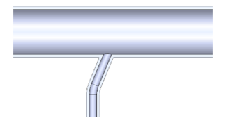
4. Side inlet enters the reaction tube at an angle of 45° Processes 09 02256 i004
5. Side inlet enters the reaction tube with a radius of 25 mm Processes 09 02256 i005
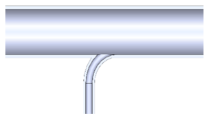
6. Side inlet enters the reaction tube with a radius of 35 mm Processes 09 02256 i006
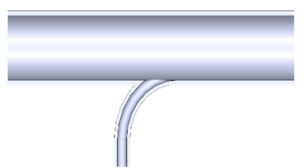
7. Side inlet enters the reaction tube in the centre of the reaction tube with a radius of 20 mm Processes 09 02256 i007
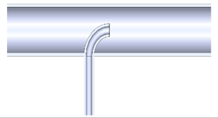
8. The shape of basic geometry, but the side inlet has a diameter of 10 mm Processes 09 02256 i008
Table 2. Flows in different simulations.
Volume Flow (L/min)Mass Flow (kg/s)
Simulation 1
H2100.00001500
N250.00010417
Simulation 2
H250.00000750
N250.00010417
Simulation 3
H250.00000750
N2100.00020833
Simulation 4
H2100.00001500
N2100.00020833
Simulation 6
H250.0000075
N2150.0003125
Table 3. Gas flows in the experiment.
Flow N2 (L/min)Flow H2 (L/min)
1.55
2.105
3.155
Table 4. Simulation results of basic geometry (blue—H2 profile, grey—N2 profile).
Selected FlowImage of the Simulation
1. Flow H2 = 5 L/min
  Flow N2 = 5 L/min
Processes 09 02256 i009
2. Flow H2 = 10 L/min
  Flow N2 = 5 L/min
Processes 09 02256 i010
3. Flow H2 = 5 L/min
  Flow N2 = 10 L/min
Processes 09 02256 i011
4. Flow H2 = 10 L/min
  Flow N2 = 10 L/min
Processes 09 02256 i012
5. Flow H2 = 5 L/min
  Flow N2 = 15 L/min
Processes 09 02256 i013
Table 5. Simulation results of different geometries (blue—H2 profile, grey—N2 profile).
The Shape of the GeometryImage of the Model
1. Side inlet at the top of the reaction tube Processes 09 02256 i014
2. Side inlet at the bottom of the reaction tube Processes 09 02256 i015
3. The side inlet enters the reaction tube at an angle of 22.5° Processes 09 02256 i016
4. The side inlet enters the reaction tube at a 45° angle Processes 09 02256 i017
5. The side inlet enters the reaction tube with a radius of 25 mm Processes 09 02256 i018
6. The side inlet enters the reaction tube with a radius of 35 mm Processes 09 02256 i019
7. The side inlet enters the reaction tube in the centre of the reaction tube with a radius of 20 mm Processes 09 02256 i020
8. The shape is of basic geometry but has a side inlet diameter of 10 mm Processes 09 02256 i021
Publisher’s Note: MDPI stays neutral with regard to jurisdictional claims in published maps and institutional affiliations.

