Abstract
High-spatiotemporal-resolution land surface temperature (LST) is a crucial parameter in various environmental monitoring. However, due to the limitation of sensor trade-off between the spatial and temporal resolutions, such data are still unavailable. Therefore, the generation and verification of such data are of great value. The spatiotemporal fusion algorithm, which can be used to improve the spatiotemporal resolution, is widely used in Landsat and MODIS data to generate Landsat-like images, but there is less exploration of combining long-time series MODIS LST and Landsat 8 LST product to generate Landsat 8-like LST. The purpose of this study is to evaluate the accuracy of the long-time series Landsat 8 LST product and the Landsat 8-like LST generated by spatiotemporal fusion. In this study, based on the Landsat 8 LST product and MODIS LST product, Landsat 8-like LST is generated using Spatial and Temporal Adaptive Reflectance Fusion Model (STARFM), Enhanced STARFM (ESTARFM), and the Flexible Spatiotemporal DAta Fusion (FSDAF) algorithm, and tested and verified in the research area located in Gansu Province, China. In this process, Landsat 8 LST product was verified based on ground measurements, and the fusion results were comprehensively evaluated based on ground measurements and actual Landsat 8 LST images. Ground measurements verification indicated that Landsat 8 LST product was highly consistent with ground measurements. The Root Mean Square Error (RMSE) was 2.862 K, and the coefficient of determination R2 was 0.952 at All stations. Good fusion results can be obtained for the three spatiotemporal algorithms, and the ground measurements verified at All stations show that R2 was more significant than 0.911. ESTARFM had the best fusion result (R2 = 0.915, RMSE = 3.661 K), which was better than STARFM (R2 = 0.911, RMSE = 3.746 K) and FSDAF (R2 = 0.912, RMSE = 3.786 K). Based on the actual Landsat 8 LST images verification, the fusion images were highly consistent with actual Landsat 8 LST images. The average RMSE of fusion images about STARFM, ESTARFM, and FSDAF were 2.608 K, 2.245 K, and 2.565 K, respectively, and ESTARFM is better than STARFM and FSDAF in most cases. Combining the above verification, the fusion results of the three algorithms were reliable and ESTARFM had the highest fusion accuracy.
1. Introduction
Land surface temperature (LST) is a key variable of the surface energy process, hydrological balance, and climate change [1,2,3,4,5]. Accurate measurement and the estimation of LST are of great significance to many research fields, such as weather forecasting, ocean circulation, drought monitoring, and energy balance [6]. At present, thermal infrared remote sensing is almost the only method for regional monitoring of LST.
However, due to the mutual restriction between spatial and temporal resolution, no satellite system can provide a thermal band or LST data with high spatial and temporal resolution at the same time [7]. Sensors with good spatial resolution show poor temporal resolution and vice versa [8]. For example, MODIS provides LST at a resolution of 1 km per day, while polar-orbiting Landsat 8 100 m every 16 days. In order to meet the fine-scale monitoring, it is necessary to combine these two types of data to obtain high spatiotemporal resolution LST.
To solve this problem, methods such as downscaling [9,10], sharpening [11,12], image fusion [13,14,15], and disaggregation [7,8] were proposed to improve the LST resolution. These methods can be divided into two categories: kernel-driven method and fusion method. The former downscales the LST through the auxiliary data of the multispectral sensor, while the latter can predict the LST of fine resolution by integrating different sensors’ time change information and neighborhood information. Among them, the kernel-driven method only improves the spatial resolution without improving the temporal resolution of the sensor at the same time [15], while the fusion method improves both the temporal and spatial resolution and has been developed rapidly in the past decade [16].
The most widely used spatiotemporal fusion method is perhaps the Spatial and Temporal Adaptive Reflectance Fusion Model (STARFM) [17], which has been widely used [18,19,20]. This method assumes that land cover types and systematic errors do not change between the start time and target time, and a coarse pixel contains only one land cover type, Landsat reflectance images of the prediction period is generated using MODIS and Landsat reflectance images of the same period combined with MODIS images of the prediction period. Due to the above assumptions, STARFM is not feasible in heterogeneous regions. Therefore, STARFM has been improved for more complex surface conditions, resulting in Spatial Temporal Adaptive Algorithm for mapping Reflectance Change (STAARCH) [21] and Enhanced STARFM (ESTARFM) [22], which respectively improves the performance of STARFM in the land cover type change and disturbance existence, and STARFM’s accuracy in heterogeneous areas. Huang et al. [23,24] proposed dictionary-pair learning methods. Although the pixels of land change can be better predicted, the shape of the ground objects cannot be maintained. Aiming at the limitations of existing spatiotemporal fusion algorithms, Zhu et al. proposed the Flexible Spatiotemporal DAta Fusion (FSDAF) [25] algorithm, which combines temporal and spatial predictions to capture gradually and suddenly land cover type changes with the need for only one high spatial resolution image. The current research and application of the FSDAF algorithm is mainly based on surface reflectance data [26,27,28,29].
Although these spatiotemporal fusion methods were originally designed for reflectance, they have also been widely used in temperature fusion. Li et al. [30] and Ma et al. [31] used the STARFM and ESTARFM algorithm to generate thermal band data for the study of evapotranspiration. Yang et al. [32] generated ASTER surface temperature based on the ESTARFM algorithm and verified it based on the ground measurements. According to the STARFM framework, Huang [33] considered the thermal effects of adjacent pixels and used a bilateral filtering algorithm to construct a new weighting function for the fusion model to monitor the urban thermal environment. Weng et al. [15] proposed the Spatial-temporal Adaptive Data Fusion Algorithm for Temperature mapping (SADFAT) algorithm for LST prediction based on the STARFM algorithm framework, considering the annual temperature cycle (ATC) and thermal landscape heterogeneity. These STARFM-like algorithms are mainly applied to two sensors. For temperature data fusion of three or more sensors, Wu et al. [13] proposed the Spatiotemporal Integrated Temperature Fusion Model (STITFM) algorithm based on the STARFM algorithm, analyzed the fusion of geostationary satellite, Landsat, and MODIS LST. However, similar to STARFM, STITFM is poorly adaptable to areas with complex surface heterogeneity and land cover type changes. Quan et al. [14] proposed a temperature fusion algorithm—Blend Spatiotemporal Temperatures (BLEST), which can be used for heterogeneous regions and land cover type changes by integrating the characteristics of existing spatiotemporal fusion algorithms [15,17,21,25], and combined Landsat, MODIS, and geostationary satellite to generate Landsat-like LST at 1 h interval.
Although the spatiotemporal fusion algorithm is widely used in the generation of high spatiotemporal resolution temperature data, however, there are still some issues that need to be explored. On one hand, previous studies mainly focused on the improvement and application of algorithms and lacked ground verification of long-time sequence fusion results. The reliability of the fusion results requires long-term sequence verification. On the other hand, in previous studies, researchers have inverted Landsat 8 LST based on thermal band data, and the steps are cumbersome. Using the standard Landsat 8 LST product can solve this problem, but there is no relevant report so far, so the reliability of using it in fusion needs to be studied. In response to the above problems, this study used MODIS LST product and Landsat 8 LST product to participate in the fusion, and used three common spatiotemporal fusion algorithms, i.e., STARFM, ESTARFM, and FSDAF, to generate long-time sequence data of 28 scenes in the study area from 2013 to 2016, and verified and analyzed the fusion results based on ground measurements LST. Since Landsat 8 LST product is rarely used and verified at present, the accuracy of the Landsat 8 LST product is also evaluated in order to have a more objective analysis of fusion results. Satellite data and ground measurement data are introduced in Section 2. In Section 3, the temperature inversion of the Landsat 8 LST product, the theoretical basis of the spatiotemporal fusion method, the fusion scheme, and the evaluation strategy are described. The evaluation results are detailed in Section 4. Finally, the discussion and conclusions of this study are summarized in Section 5 and Section 6.
2. Study Area and Data
2.1. Study Area
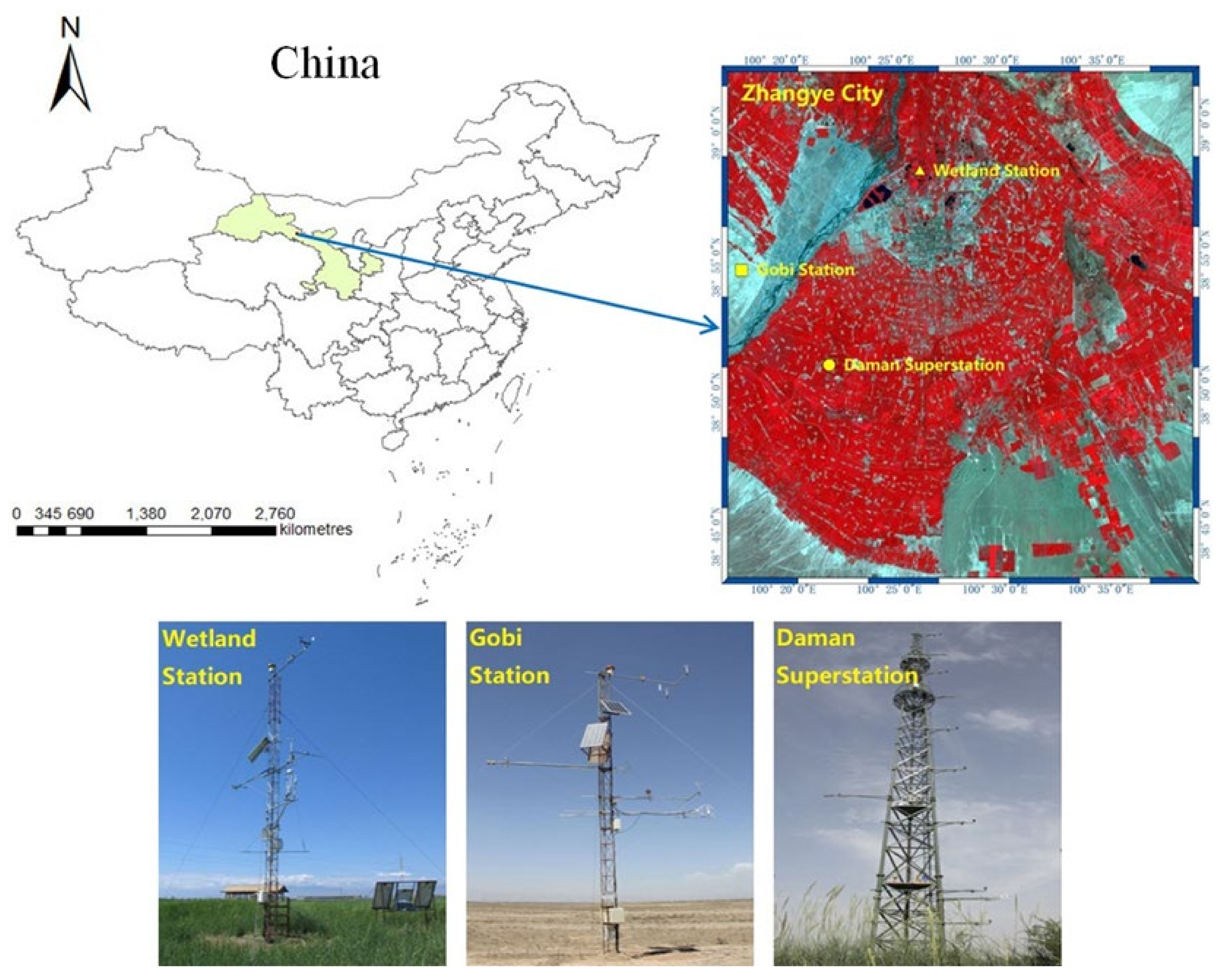
The study area is located in Zhangye City, Gansu Province, China, which belongs to the midstream of the Heihe River Basin, with a geographic range of 38°43′15.60″–39°02′16.8″ N, 100°17′45.59″–100°39′21.59″ E. The climate in this area is arid, with an average annual temperature of 7 °C, and the area has obvious characteristics of the four seasons. The average temperature in summer (June to August) is 20 °C; the winter is cold (December to February) with an average temperature of −8 °C; the temperature rises faster in spring (March to May) with an average temperature of 9 °C; and in autumn (September to November), the temperature drops quickly with an average temperature of 7 °C. Here July is the hottest and January is the coldest. The area is flat and the primary land cover is farmland, Gobi, sandy land, forest, water area, and buildings, most of which are farmland and Gobi. The main crops grown in farmland are spring wheat, corn, barley, flax, and so on. The location of the study area and stations is shown in Figure 1.
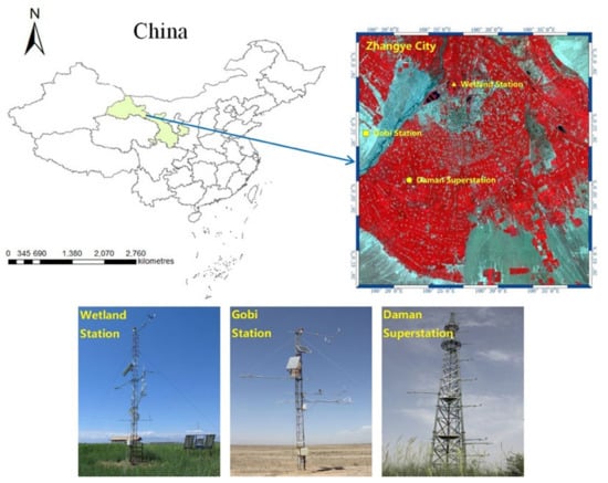
Figure 1.
Location of the study area and stations’ spatial distribution.
2.2. Data
2.2.1. MODIS and Landsat 8 Data
The Landsat 8 LST product from Landsat 8 collection 2 level-2 data (downloaded from https://earthexplorer.usgs.gov/ accessed on 9 November 2021). in this study has an overpass time, which is approximately 10:55 a.m. at local solar time, and a revisiting period of 16 days. The spatial resolution of the TIR channel is 100 m (note: downloaded images are provided with 30 m), with 30 pieces of Landsat 8 scene data of Path 133, Row 33 without cloud collected in the study area from 2013 to 2016. The Landsat 8 LST product provides a basis for the wide application of the Landsat8 thermal band. The corresponding daily MODIS datasets (downloaded from https://ladsweb.modaps.eosdis.nasa.gov/search/ accessed on 9 November 2021) include MOD11A1 (1 km MODIS LST product) and MOD05_L2. MOD11A1 was retrieved by a generalized split-window algorithm [34], and in most cases, the accuracy was reported within 2.0 K [35]. The MOD05_L2 product contains 1 and 5 km atmospheric column water vapor (CWV) [36]; in this study, 1 km CWV data generated by the near-infrared algorithm are used. The overpass time is approximately 11:40 a.m. at the local solar time for MOD11A1 and MOD05_L2 in this study area.
Before implementing the fusion method, both the Landsat 8 and MODIS data are registered to the same coordinate system and resampled to the exact spatial resolution (using a nearest-neighbor method). Since Landsat 8 LST product is provided at 30 m, the MODIS is resampled to 30 m resolution (note: the actual resolution of Landsat 8 LST is 100 m).
2.2.2. Ground Measurements LST
The ground measurements are from HiWATER: Dataset of hydrometeorological observation network [37,38]. The observation data of three automatic weather stations-Zhangye wetland station, Bajitan Gobi station, and Daman superstation-are used in this study. The details of the three verification stations are shown in Table 1. The observation frequency of the automatic weather station is 30 s, and the output is average data of 10 min. According to the Landsat 8 satellite transit time, data within 10 min are linearly interpolated to estimate the measured value of the satellite transit time. Surface radiometric temperature is observed by SI-111 radiometers (8–14 um) installed in the automatic weather station. The true land surface temperature can be obtained by Equation (1):
where is the Planck function, ε the surface emissivity of the SI-111 channel calculated by ASTER GEDv3, and the atmospheric downward radiation measured by the SI-111.

Table 1.
Verifying station information.
3. Methodology
3.1. Landsat 8 LST Retrieval
The global standard Landsat 8 LST product is used in this study, which is based on the inversion of TIR10 and has been used since mid-2020. Firstly, the temperature retrieval process involves calculating ground radiance using emissivity, atmospheric parameters, and the observed Landsat 8 radiance for band 10, and then inverting the Planck function.
where is the LST, the Planck function at temperature ; represents the Top of the Atmosphere (TOA) radiance received by the TIR sensor, the surface emissivity, , and upwelling atmospheric radiance, downwelling atmospheric radiance, and atmospheric transmittance, respectively, and the effective band wavelength; and are Planck’s radiation constants with value 1.19104 × 10⁸ W·μm4·m−2·sr−1 and 14,387.7 μm·K, respectively.
Theoretically, the surface temperature can be obtained by inverting the Planck function in Formula (3) and combining in Formula (2) as follows:
However, this formulation will increasingly become inaccurate for a sensor’s spectral response that deviates from delta function behavior. Instead, use a lookup table (LUT) to calculate Landsat 8 LST. Calculate the expected radiances of the spectral response of Landsat 8 sensor in the temperature range of 0.01 K, which encompasses all expected Earthlike temperatures (typically 150–380 K). This results in a table of values of radiances versus temperatures for Landsat 8 sensor. Landsat 8 LST can be retrieved by using the ground radiance and the table. For a more detailed description of the Landsat 8 LST product, please refer to Malakar et al. (2018) [39].
3.2. Introduction of Spatial Temporal Fusion Models
The STARFM [17] algorithm is the most widely used spatiotemporal fusion algorithm and uses a pair of high/low-resolution images at the reference time and a low-resolution image at the target time to fuse. The moving window and similar pixels are introduced during fusion to reduce the influence of the pixel boundary of low spatial resolution images, using similar pixels in the window and comprehensively considering the spatial weight, spectral weight and temporal weight to calculate the value of the center pixel in the window, and finally predicting the high-resolution image of the target time through the movement of the moving window.
The ESTARFM [22] algorithm, which is improved on the basis of STARFM, introduces a conversion coefficient to improve the accuracy of STARFM in heterogeneous regions. When the ESTARFM model is fused, it is necessary to input two pairs of high/low-resolution images at the reference time and a low-resolution image at the target time. Similar to STARFM, ESTARFM still uses the moving window technology, which uses similar pixels in the window and comprehensively considers the weight function to solve the value of the center pixel to realize the prediction of the high-resolution image at the target time.
The FSDAF [25] algorithm is an unmixing-based fusion model, which can predict the gradual changes and mutations of land cover types. The input data of the algorithm are the same as those of STARFM. First, the time change information is obtained through the pure pixels of the low-resolution images at time t1 and t2 that have not changed the ground cover, and then the time-predicted high-resolution image is obtained. The spatially-predicted high-resolution image is obtained by increasing the image resolution through the thin-plate spline interpolation function so as to obtain the residual R of each lower resolution pixel on the prediction date. Finally, the distribution weight function is used to assign the residuals, and this function generates the final target image by using similar pixels similar to STARFM and ESTARFM to reduce the blocking effect.
3.3. Fusion Scheme
The following two kinds of data need to be input for temperature fusion: reference images, namely Landsat 8 LST and MODIS LST images of the same date, and MODIS LST image of the predicted date. When the predicted date is determined, the selection of the reference images has a great impact on the prediction results. Generally, the date adjacent to the predicted date is used as the reference image date under which circumstance the temperature change, surface coverage type change, and sensor difference change between reference and predicted images are small, which is helpful to improve the prediction accuracy. A pair of reference images are required for STARFM and FSDAF, however, for the predicted date, there are two adjacent dates, involving two pairs of reference images. The dates of the reference images are selected by comparing the coefficient of determination (R2) between the MODIS LST images of the two dates and the MODIS LST images at the predicted date, and the date with higher correlation is used as the reference image date. Two pairs of reference images are required for ESTARFM, and the adjacent dates of the predicted date are directly selected. The fusion scheme is shown in Figure 2. T1 represents the reference image date of STARFM and FSDAF, T1 and T3 ESTARFM, and T2 represents the fusion image date.

Figure 2.
The scheme for estimation of Landsat 8-like LST by STARFM, ESTARFM, and FSDAF.
3.4. Verification and Evaluation
The Landsat 8 LST product is verified based on ground measurements, and the fusion results are comprehensively evaluated based on the ground measurements and the actual Landsat 8 LST images. The prediction accuracy is evaluated with the coefficient of determination (R2), mean difference (bias), mean absolute error (MAE), and root mean square error (RMSE). The statistical metrics are given as follows:
where is the number of observations, and are the verified and estimated LST, respectively.
4. Results
4.1. Test Landsat 8 LST with Ground Measurements
The Landsat 8 LST product became available in mid-2020. At present, few applications and verifications are available for this product, and when generating Landsat-like LST based on the spatiotemporal fusion algorithm, many scholars [13,14,15,40] used single-channel (SC) algorithm proposed by Jiménez-Muñoz et al. [41,42,43] to estimates the Landsat LST. Therefore, it is necessary to verify the Landsat 8 LST product before fusion. In this study, Landsat 8 LST product was verified based on ground measurements and compared with the SC algorithm. In the SC algorithm for Landsat 8, which is not described here, the emissivity comes from the emissivity band in Landsat 8 Collection 2 Level-2 data, and the water vapor comes from the MOD05_L2 product. For the detailed algorithm flow, please refer to Jiménez-Muñoz et al. (2014) [43].
It is necessary to analyze the heterogeneity of the ground station before using ground measurements LST. Generally, 3 × 3 pixel LST around the station is counted due to the Landsat 8 LST product is provided with the resolution resampled to 30 m, but the actual resolution is 100 m, so 9 × 9 pixel (270 m) around the station was counted in this study, and the average standard deviation of all 30 Landsat 8 LST scene images was calculated as the basis for site heterogeneity analysis. The statistical results show that the average standard deviations of the Wetland station, Gobi station, and Daman superstation are 0.864 K, 0.411 K, and 0.485 K, respectively, which are all less than 1 K. It meets the requirement that the uncertainty of the ideal surface temperature verification site should be within 1 K, as pointed out by Wan et al. [44].
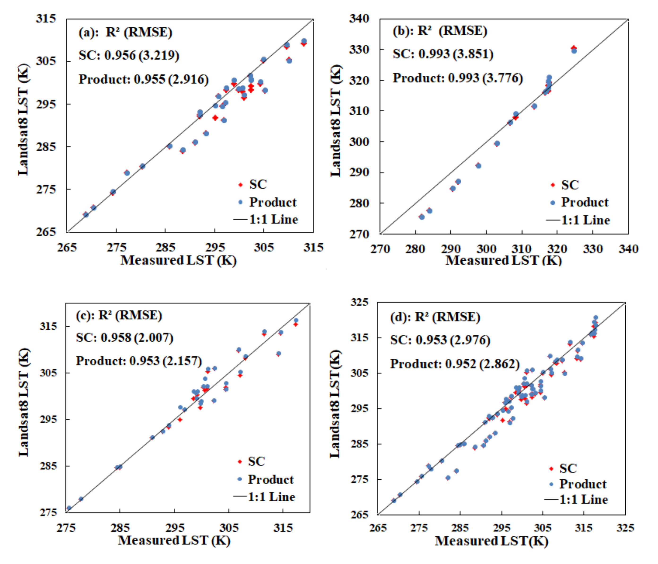
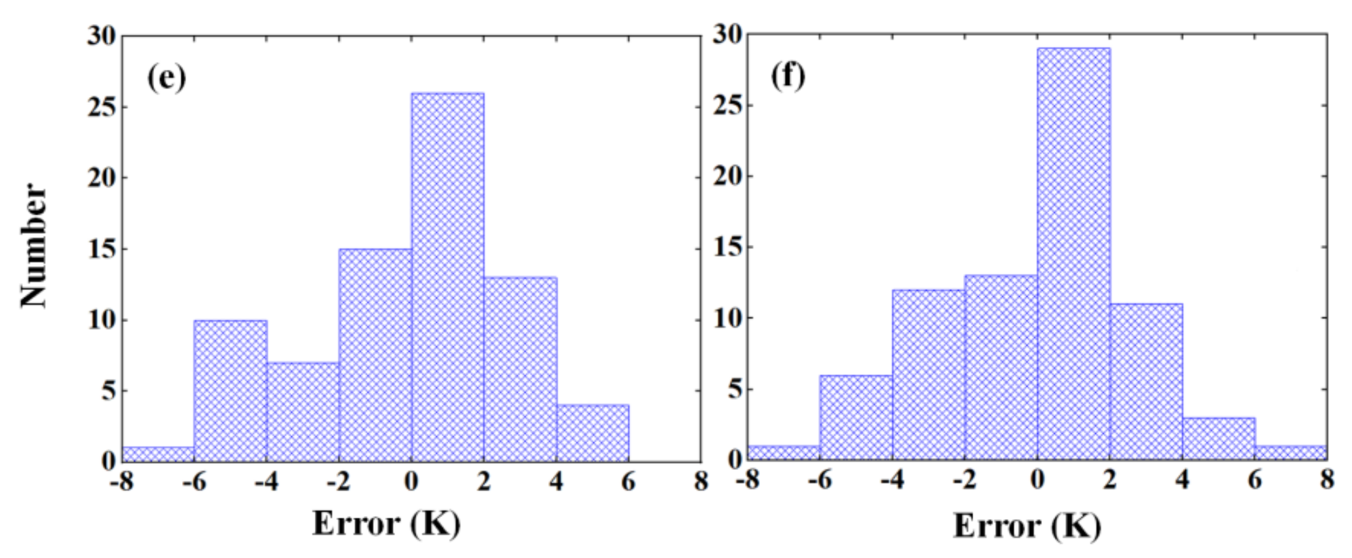
According to the ground measurements at different sites, the bias, MAE, and RMSE of the SC LST and LST product are listed in Table 2. At the Wetland and Gobi station, LST product RMSE are 2.916 K and 3.776 K, respectively, which are smaller than that of SC LST (3.219 K and 3.851 K, respectively). At Daman superstation, the two types of LST RMSE are close to 2 K with 2.157 K of LST product and 2.007 K of SC LST. All stations represent the comprehensive verification results of the three stations; the LST accuracy of these two algorithms in All stations is within 3 K, and the accuracy of the LST product is slightly better than that of the SC LST. The comparison between SC LST and LST product is shown in Figure 3, the two types of LST are highly linearly related to ground-measured LST with R2 greater than 0.953, and the R2 of LST product and SC LST are very close at each site. The histogram distribution of the LST differences between retrieved and measured LST shows that for the two types of LST, most biases are between −3 K and 3 K, and the overall bias of LST product and SC LST at All stations are −0.760 K and −1.284 K, respectively. LST product has reliable accuracy and is suitable for input data in spatiotemporal fusion based on the above verification.

Table 2.
The bias (K), MAE (K), and RMSE (K) of retrieved LST over stations.
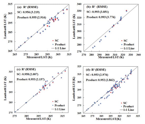
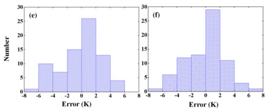
Figure 3.
Scatter plot and error histogram of retrieved LST and measured LST. (a): Wetland station; (b): Gobi station; (c): Daman superstation; (d): All stations; (e): LST product error histogram at All stations; (f): SC error histogram at All stations.
4.2. Test Fusion Data with Ground Measurements and Actual Landsat 8 LST Product
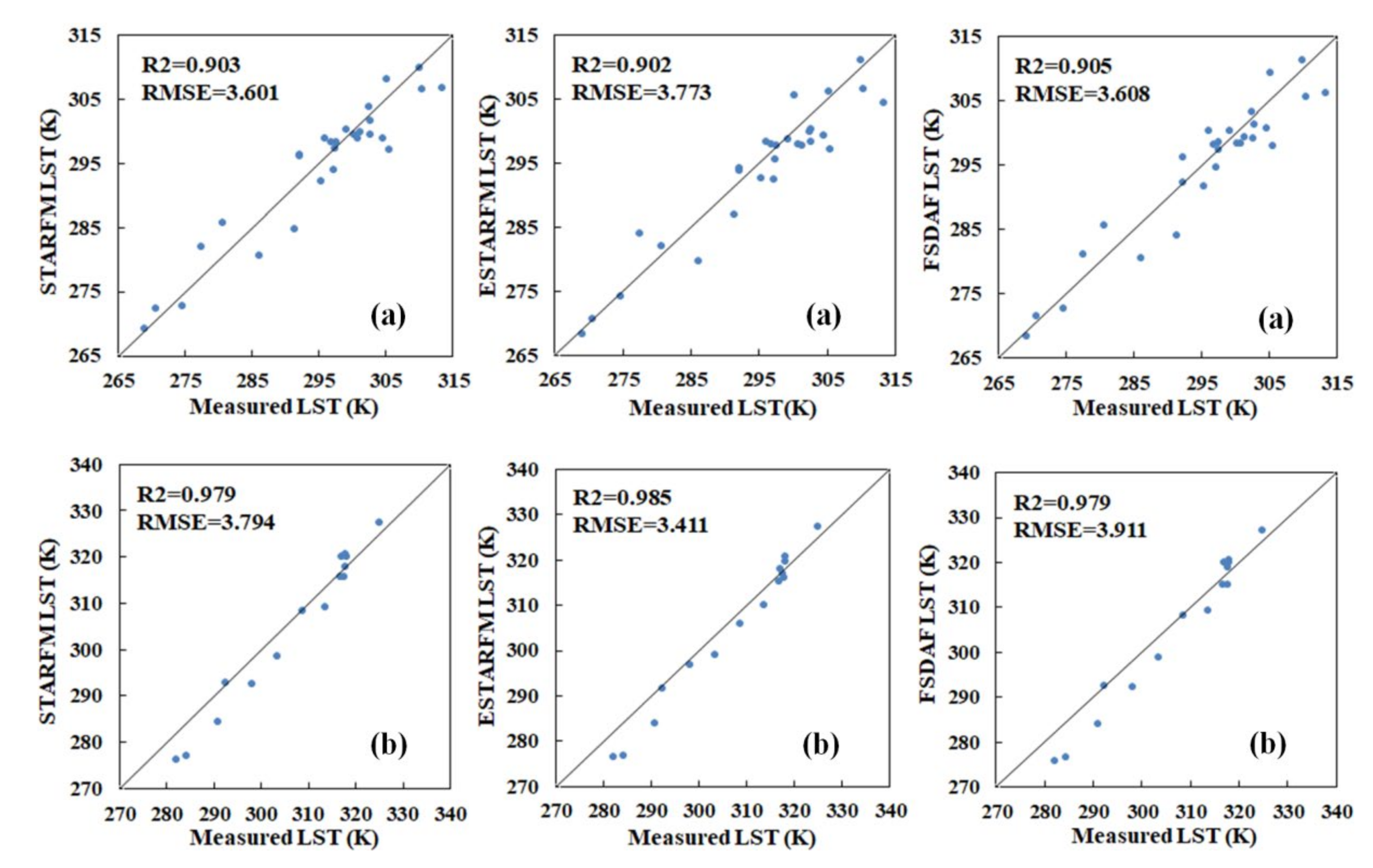
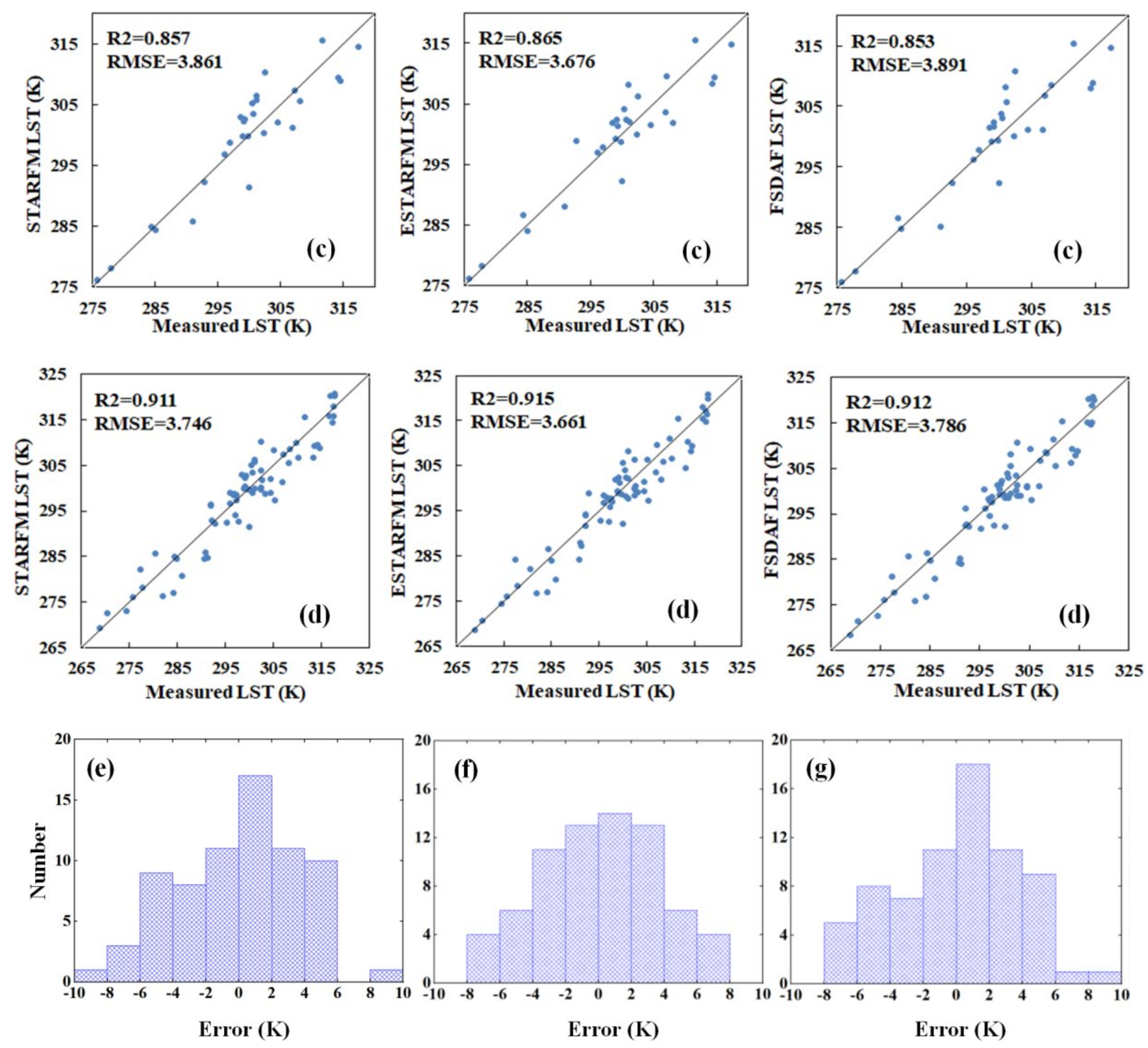
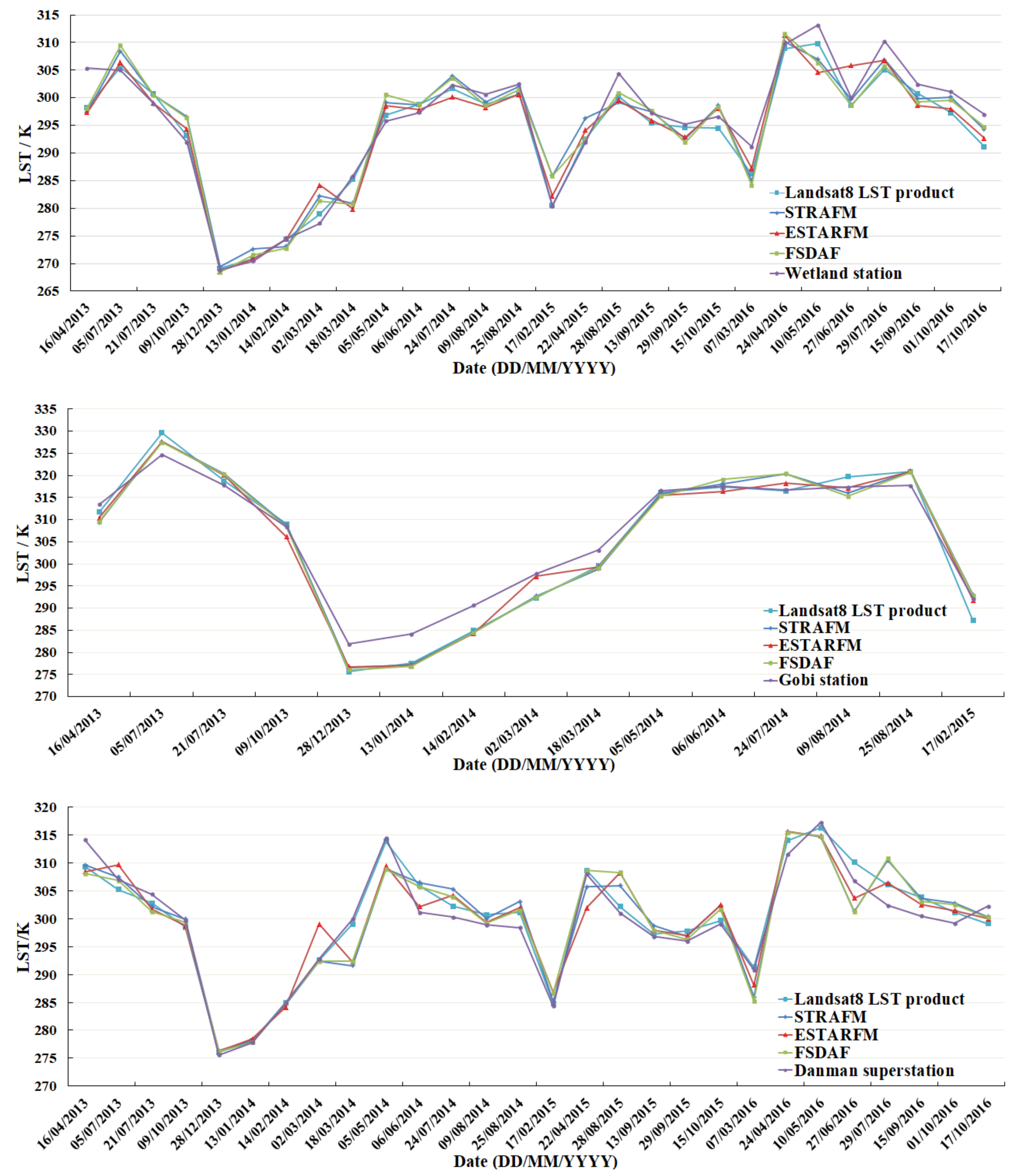
Twenty-eight Landsat 8-like LST scene images are generated according to the fusion scheme of Figure 2. The comparison of the ground measurements and fusion results at the site is shown in Figure 4 and Figure 5. The fusion results of the three algorithms are highly consistent with the ground measurements, and R2 is greater than 0.853 (Figure 4). In addition to the Wetland station, ESTARFM has a higher correlation with measured LST at the remaining stations compared with STARFM and FSDAF. From the perspective of All stations, the R2 of STARFM, ESTARFM, and FSDAF is 0.911, 0.915, and 0.912, respectively. The R2 of Gobi station is larger than that of Wetland station and Daman superstation, for the surface coverage of Gobi Station is almost unchanged over time.
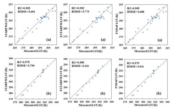
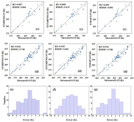
Figure 4.
Scatter plot and error histogram of fused LST and measured LST. (a): Wetland station; (b): Gobi station; (c): Daman superstation; (d): All stations; (e): STARFM error histogram at All stations; (f): ESTARFM error histogram at All stations; (g): FSDAF error histogram at All stations.
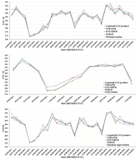
Figure 5.
Time series comparison of fused and measured LST.
The results of the correlation analysis between the fusion LST and the ground measurements are shown in Table 3. By analyzing evaluation indicators from All stations, it is found that ESTARFM (MAE = 2.965 K, RMSE = 3.661 K) is less than STARFM (MAE = 3.064 K, RMSE = 3.746 K) and FSDAF (MAE = 3.065 K, RMSE = 3.786 K). Based on the analysis of a single site, except for the Wetland station, ESTARFM performed better than STARFM and FSDAF on the other two sites. For bias, although ESTARFM (bias = −0.607 K) is greater than STARFM (bias = −0.274 K) and FSDAF (bias = −0.470 K), it is closer to Landsat 8 LST product (bias = −0.760 K), STARFM and FSDAF show too small deviations, which may be caused by error propagation in the fusion. The histogram distribution of the LST differences between the fused and measured LST shows most biases are between −4 K and 4 K (Figure 4e–g). Comprehensive analysis shows that ESTARFM fusion results are slightly better than STARFM and FSDAF at the site.

Table 3.
The bias (K), MAE (K), and RMSE (K) of fused LST over stations.
In order to analyze the fusion results of the three algorithms in more detail, the predicted Landsat 8-like LST images are evaluated from the correlation analysis and visual interpretation based on actual Landsat 8 LST images as the verification data. In the study area, some MODIS LST images have default data (the value is 0), and errors will be brought into the fusion results. Therefore, when evaluating the images of the study area, these fused images with errors will be eliminated.
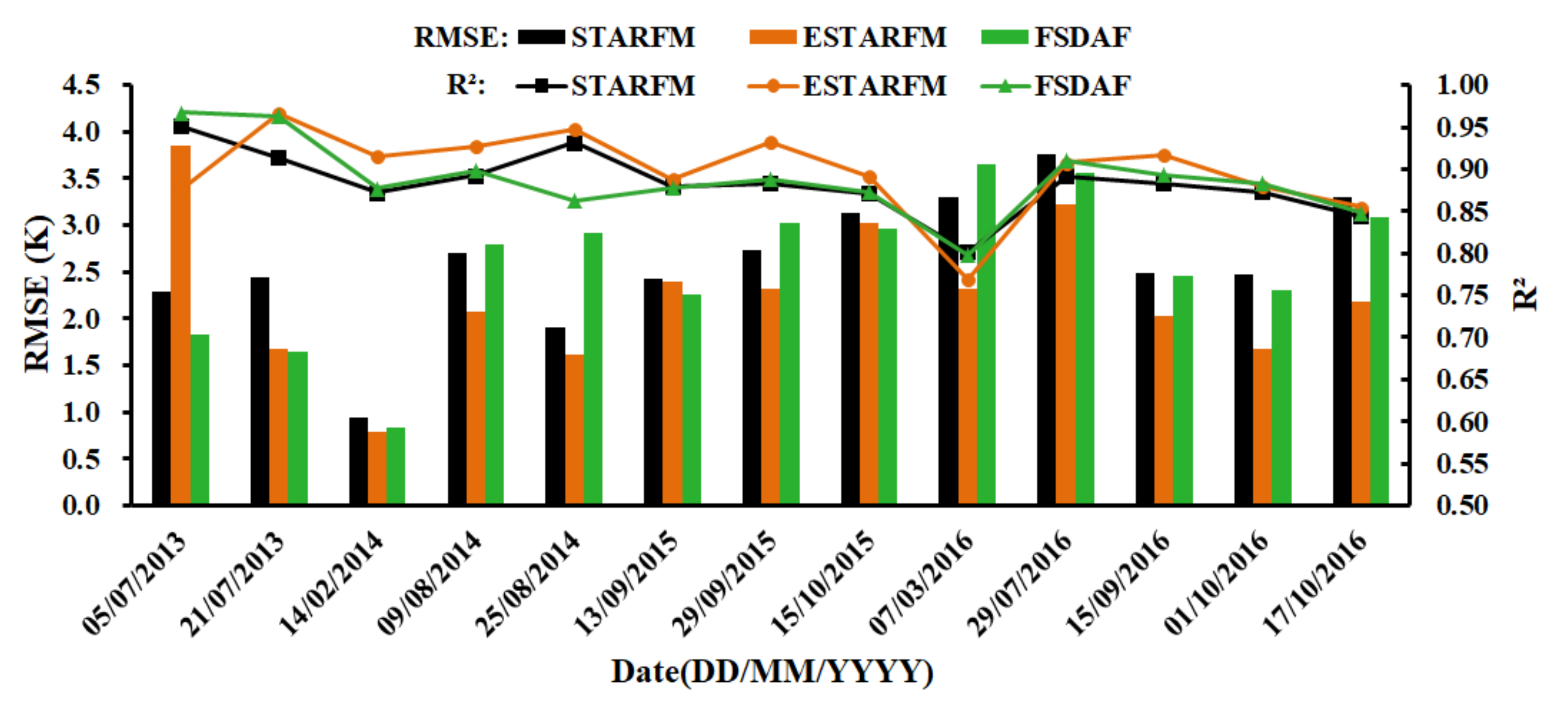
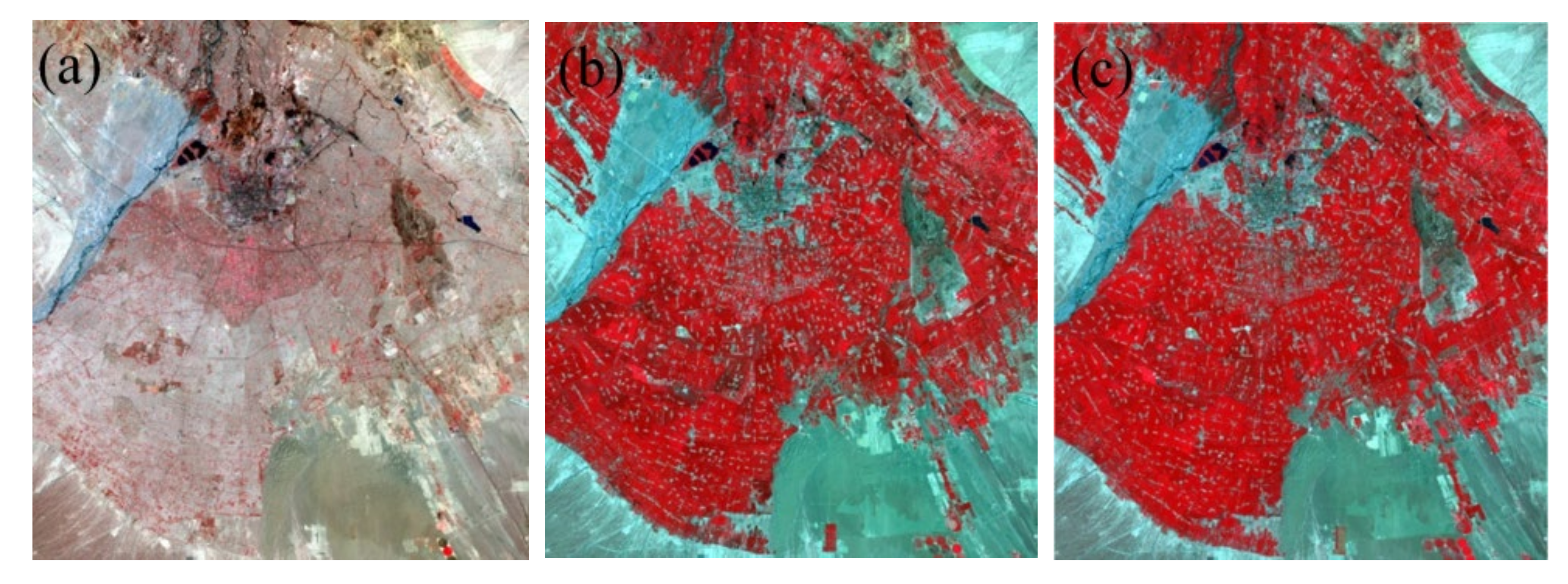
The correlation analysis results between fused images and the actual Landsat 8 LST images are shown in Figure 6. It can be seen that the Landsat 8 LST images generated by all three fusion methods are very similar to the actual images, and R2 is higher than 0.769. In most cases, the R2 of ESTARFM is larger and RMSE is smaller compared with STARFM and FSDAF. After calculating, the average R2 of the fusion data of STARFM, ESTARFM, and FSDAF were 0.883, 0.898, 0.888, and the RMSE were 2.608 K, 2.245 K, and 2.565 K, respectively. ESTARFM evaluation index is better than STARFM and FSDAF. However, the RMSE of ESTARFM on 5 July 2013 was 3.846 K, which was significantly greater than that of STARFM and FSDAF. The main reason is that compared with STARFM and FSDAF, the image of 16 April 2013 was added for ESTARFM in the fusion process. The reason for the errors were introduced is that large land cover difference between 16 April 2013 (Figure 7a) and 5 June 2013 (Figure 7b), which should be paid attention to when using ESTARFM algorithm.
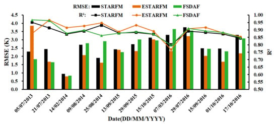
Figure 6.
The R2 and RMSE (K) of fused LST images and actual LST images.
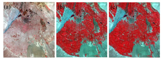
Figure 7.
Landsat 8 standard false color image (a): 16 April 2013; (b): 5 June 2013; (c): 21 June 2013.
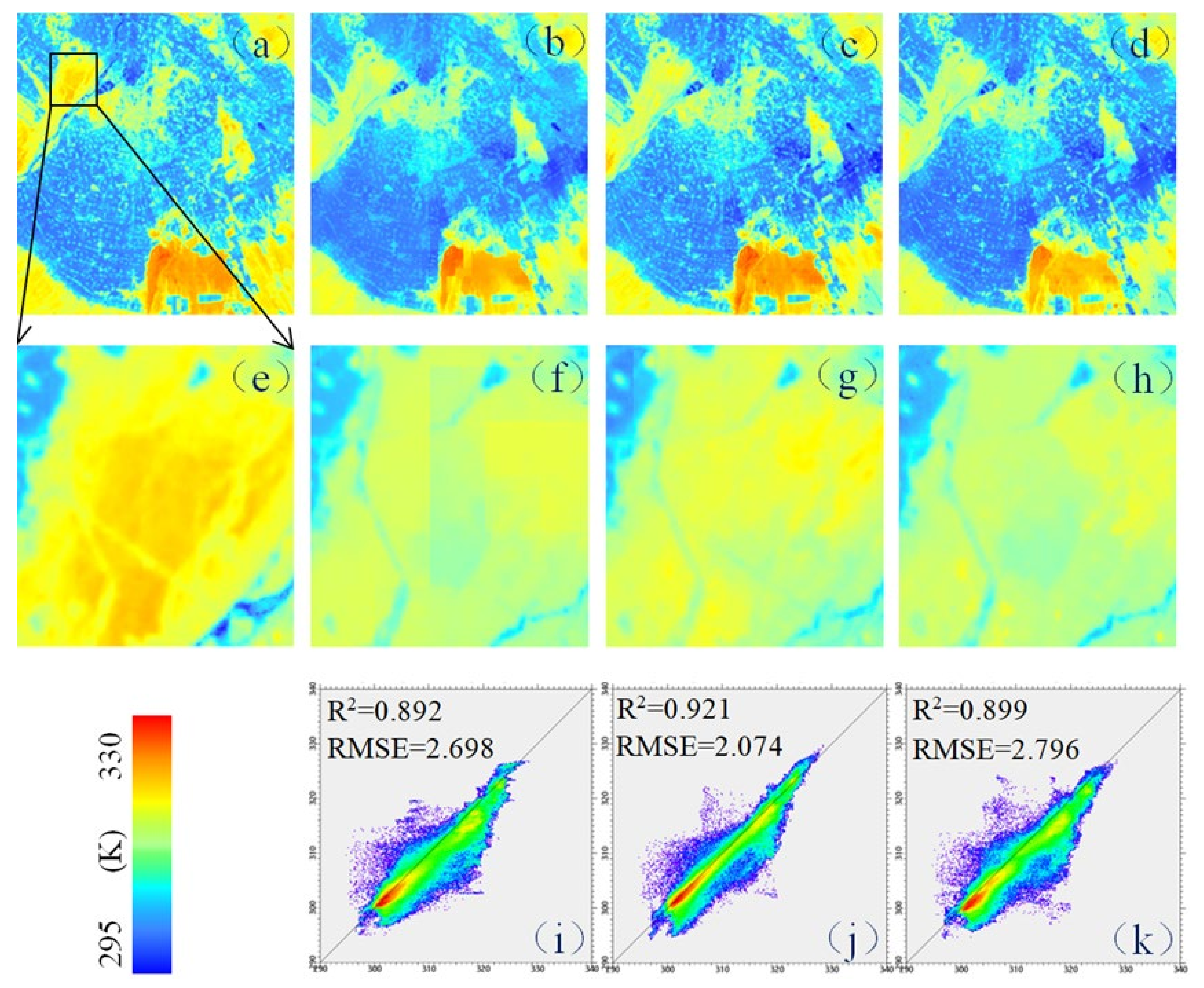
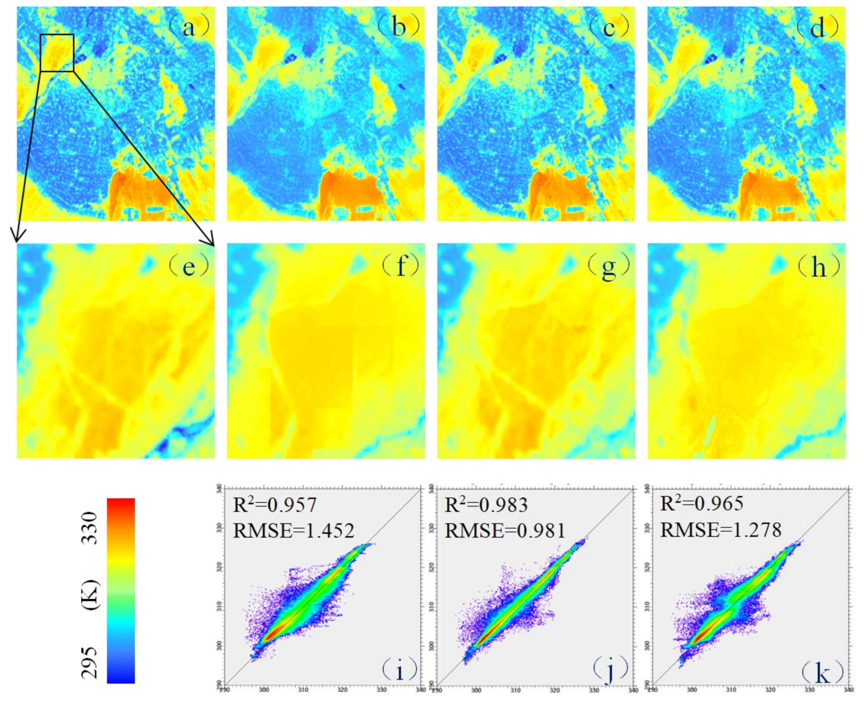
The visual interpretation results between the fused images and the actual Landsat 8 LST images on 9 August 2014 are obtained from Figure 8 and Figure 9. From the overall image (Figure 8b–d), the fusion result of ESTARFM and FSDAF is clearer than that of STARFM. In the subset (Figure 8e–h), the spatial detail of ESTARFM is the closest to the actual Landsat 8 LST, followed by FSDAF, and the STARFM result is the worst. However, for the fusion results of all three algorithms, the temperature was underestimated compared with the actual Landsat 8 LST. After analysis, it can be inferred that the cause is radiometric and geometric inconsistencies between the two sensors. The low-resolution data use simulated MODIS LST (resampled to 1000m based on Landsat 8 LST) in Figure 9, there is no underestimation in the subset, and the overall fusion accuracy has been improved. It can be seen that ESTRAFM still has the best fusion effect, which is the closest to the actual Landsat 8 LST, followed by FSDAF, and then STARFM.
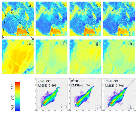
Figure 8.
Results of fusing MODIS LST and Landsat 8 LST on 9 August 2014. (a): Actual Landsat 8 LST; (b): STARFM LST; (c): ESTARFM LST; (d): FSDAF LST; (e–h): the subsets of (a–d) corresponding to the blacks quare area in (a). (i–k): scatter plot between (a–d).

Figure 9.
Results of fusing simulated MODIS LST and Landsat 8 LST on 9 August 2014. (a): Actual Landsat 8 LST; (b): STARFM LST; (c): ESTARFM LST; (d): FSDAF LST; (e–h): the subsets of (a–d) corresponding to the black square area in (a). (i–k): scatter plot between (a) and (b–d).
From the analysis of the above results, ESTARFM shows the best performance in most cases, whether it is verified from the ground site or based on the actual Landsat 8 LST image. However, when there is a large land cover difference between the reference and predicted images, errors will be introduced instead, and attention needs to be paid when performing ESTARFM fusion. The STARFM fusion images are blurry, and the spatial details are not as good as FSDAF. It is worth noting that the three algorithms will be affected by the difference between high- and low-resolution data, which can be seen by comparing Figure 8 and Figure 9.
5. Discussion
In this study, the Landsat 8 LST product and the results of spatiotemporal fusion are analyzed and verified for a long time series. The accuracy of Landsat 8 LST product is better than that of SC LST, and it has a strong correlation with ground measurements. STARFM, ESTARFM, and FSDAF algorithms can all be used to generate Landsat 8-like LST that is highly correlated with the actual Landsat 8 LST. However, in the application of these methods, there are still problems that need to be solved.
5.1. Lack of Landsat 8 LST Product Verification in High Water Vapor Content
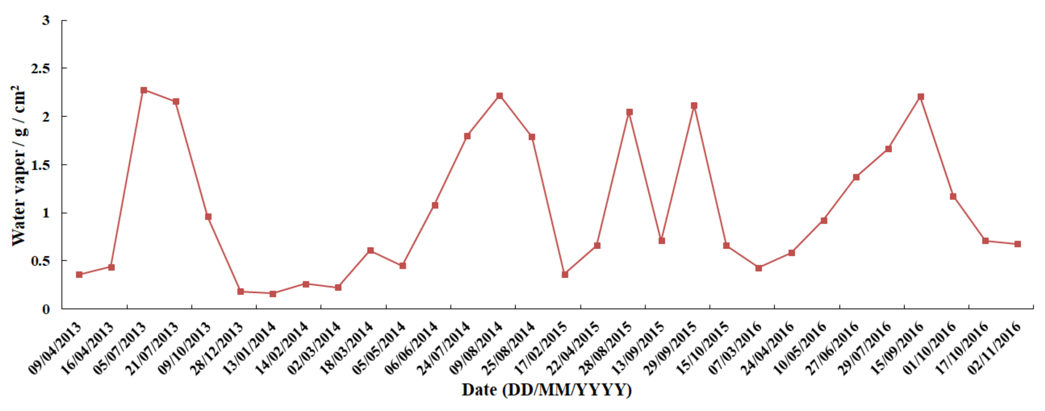
In this article, the Landsat 8 LST product in the study area was verified. From Figure 3, it can be seen that R2 at All stations is 0.952, and most of the deviations are between −3 K and 3 K, which have high accuracy. However, the atmospheric water vapor content in this study area is relatively low, less than 2 g/cm2 on most days. Figure 10 shows the average value of atmospheric water vapor content in the study area (from MOD05_L2). The case of high water vapor content has not been verified, and it is necessary to consider conducting comparative verification in areas with high water vapor content in future studies.
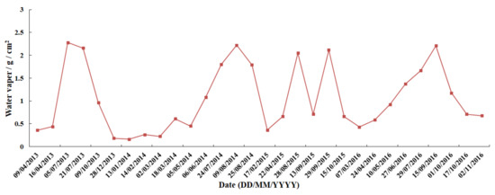
Figure 10.
Atmospheric water vapor content in the study area.
5.2. Differences in High- and Low-Resolution Data
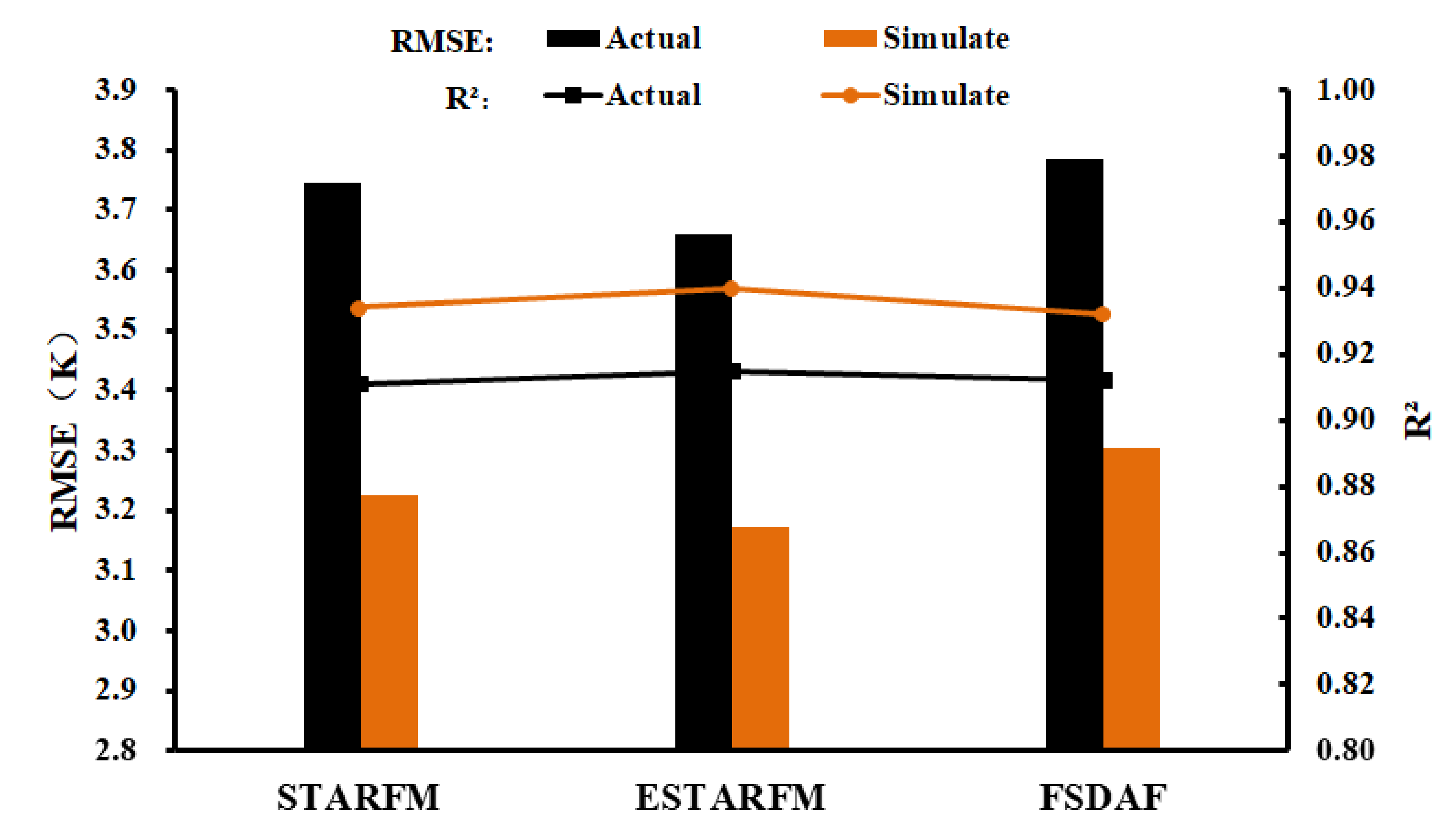
From the comparison of Figure 8 and Figure 9, it can be seen that replacing the actual MODIS LST with the simulated MODIS LST will improve the accuracy of the fusion results and have better spatial details. This is mainly because the simulated MODIS LST is based on Landsat 8 LST resampling, which is more consistent with the actual Landsat 8 LST and avoids errors caused by different differences between sensors, satellite angles, and temperature retrieval algorithms. The fusion results of simulated and actual MODIS LST are verified based on ground measurements (Figure 11). The fusion accuracy of the three algorithms has been improved when using simulated MODIS LST, and the RMSE is reduced by about 0.5 K, so improving the consistency of the Landsat 8 LST and MODIS LST images is a problem that needs to be explored.

Figure 11.
Comparison of simulation and actual fusion results over stations.
5.3. Uncertainty of STARFM, ESTARFM, and FSDAF Input Parameters
The three spatiotemporal fusion algorithms contain the following two important parameters: the number of land cover types and the size of the search window. The former is set to 4, while the latter 2 × 2 MODIS pixel in this study. However, the number of land cover types and spatial heterogeneity in the study area will change over time, especially in the study of long time series. It is necessary to adjust the amount of land cover and the size of the search window according to the actual situation of the study area. How to automatically optimize these two parameters during fusion is a question that needs to be studied in the next step.
5.4. Selection of Reference Images
Only one high-resolution reference image is required for STARFM and FSDAF, while two are required for ESTARFM. Errors may be introduced by the additional reference images. For example, when the situation shown in Figure 7 occurs, the difference in surface coverage between the two high-resolution reference images is large, which seriously affects the ESTARFM fusion result. Therefore, it is necessary to fully consider the conditions of the reference image when using the ESTARFM fusion algorithm.
5.5. MODIS LST Noise
There is noise in MODIS LST data, and the noise error will be introduced into the fusion result. Due to the influence of noise, only 13 scene fusion images are used in the accuracy evaluation based on the actual images (Figure 6). Therefore, noise removal should be performed on MODS LST before fusion to ensure the reliability of the fusion image.
In this study, the three algorithms of STARFM, ESTARFM, and FSDSAF are compared and verified. The original application scenarios of these algorithms are the fusion of surface reflectance data, and the temperature change characteristics are not considered. At the same time, some researchers combined the annual temperature cycle (ATC) [14,15] model with the spatiotemporal fusion algorithm. However, considering the ATC model cannot describe specific daily surface temperature characteristics, which leads to the uncertainty of the model, this kind of fusion algorithm is not validated in this article.
6. Conclusions
In this study, we applied the Landsat 8 LST product to the fusion, and evaluated the accuracy of the Landsat 8 LST product and the fusion results of STARFM, ESTARFM, and FSDAF.
We used ground measurements LST to verify Landsat 8 LST product. The results indicated that Landsat 8 LST product is highly correlated with ground measurements, and accuracy over All stations of LST product (bias = −0.760 K, RMSE = 2.862 K) is better than that of SC algorithm (bias = −1.284 K, RMSE = 2.967 K). The use of this standard product avoids the LST inversion before the fusion and makes the Landsat 8 thermal band more widely used.
The three algorithms of STARFM, ESTARFM, and FSDAF were comprehensively evaluated based on the ground measurements and actual Landsat 8 LST images. The verification results based on the ground measurements show that in All stations, the R2 of the three algorithms is greater than 0.911 and the MAE is less than 3.065 K, the smallest with MAE of ESTARFM, which is 2.965 K, followed by STARFM 3.064 K and then FSDAF 3.065 K. Based on the actual Landsat 8 LST images as the verification data, the R2 of the three algorithms for the 13 scene fusion images is all greater than 0.769, which has a high correlation with the actual Landsat 8 LST images. The evaluation index of MAE and RMSE (the average of the 13 scene fusion images) shows ESTARFM (MAE = 1.771 K, RMSE = 2.245 K) is smaller than STARFM (MAE = 2.129 K, RMSE = 2.608 K) and FSDAF (MAE = 2.077 K, RMSE = 2.565 K). In the 13 scene fusion images, ESTARFM is better than STARFM and FSDAF in most cases (Figure 6). From the perspective of the spatial details of the fusion results (Figure 8 and Figure 9), ESTARFM has the best fusion effect, followed by FSDAF, and the STARFM fusion results are relatively fuzzy. The results of integrating ground measurements verification and actual Landsat 8 images verification indicated the reliability of the three algorithms and proved that ESTARFM performs best in this study.
Author Contributions
S.L. and J.W. conceived and designed the experiments; S.L. performed the experiments; D.L. and Z.R. contributed with data processing and analysis; B.Y. checked the experimental results; S.L. wrote the paper; and J.W. revised the manuscript. All authors have read and agreed to the published version of the manuscript.
Funding
This research received no external funding.
Institutional Review Board Statement
Not applicable.
Informed Consent Statement
Not applicable.
Data Availability Statement
Not applicable.
Conflicts of Interest
The authors declare no conflict of interest.
References
- Li, Z.L.; Tang, B.H.; Wu, H.; Ren, H.; Yan, G.; Wan, Z.; Trigo, I.F.; Sobrino, J.A. Satellite-derived land surface temperature: Current status and perspectives. Remote Sens. Environ. 2013, 131, 14–37. [Google Scholar] [CrossRef] [Green Version]
- Eleftheriou, D.; Kiachidis, K.; Kalmintzis, G.; Kalea, A.; Bantasis, C.; Koumadoraki, P.; Spathara, M.E.; Tsolaki, A.; Tzampazidou, M.I.; Gemitzi, A. Determination of annual and seasonal daytime and nighttime trends of MODIS LST over Greece-climate change implications. Sci. Total Environ. 2018, 616, 937–947. [Google Scholar] [CrossRef]
- Shamir, E.; Georgakakos, K.P. MODIS Land Surface Temperature as an index of surface air temperature for operational snowpack estimation. Remote Sens. Environ. 2014, 152, 83–98. [Google Scholar] [CrossRef]
- Anderson, M.C.; Kustas, W.P.; Norman, J.M.; Hain, C.R.; Mecikalski, J.R.; Schultz, L. Mapping daily evapotranspiration at field to global scales using geostationary and polar orbiting satellite imagery. Hydrol. Earth Syst. Sci. Discuss 2010, 7, 5957–5990. [Google Scholar]
- Coll, C.; Valor, E.; Galve, J.M.; Mira, M.; Bisquert, M.; García-Santos, V.; Caselles, E.; Caselles, V. Long-term accuracy assessment of land surface temperatures derived from the Advanced Along-Track Scanning Radiometer. Remote Sens. Environ. 2012, 116, 211–225. [Google Scholar] [CrossRef]
- Li, Z.L.; Duan, S.B.; Tang, B.H.; Wu, H.; Ren, H.Z.; Yan, G.J.; Tang, R.L.; Leng, P. Review of methods for land surface temperature derived from thermal infrared remotely sensed data. J. Remote Sens. 2016, 20, 899–920. [Google Scholar]
- Zhan, W.; Chen, Y.; Zhou, J.; Wang, J.; Liu, W.; Voogt, J.; Zhu, X.; Quan, J.; Li, J. Disaggregation of remotely sensed land surface temperature: Literature survey, taxonomy, issues, and caveats. Remote Sens. Environ. 2013, 131, 119–139. [Google Scholar] [CrossRef]
- Zhan, W.; Huang, F.; Quan, J.; Zhu, X.; Gao, L.; Zhou, J.; Ju, W. Disaggregation of remotely sensed land surface temperature: A new dynamic methodology. J. Geophys. Res.-Atmos. 2016, 121, 538–554. [Google Scholar] [CrossRef]
- Liu, D.; Pu, R. Downscaling Thermal Infrared Radiance for Subpixel Land Surface Temperature Retrieval. Sensors 2008, 8, 2695–2706. [Google Scholar] [CrossRef] [Green Version]
- Stathopoulou, M.; Cartalis, C. Downscaling AVHRR land surface temperatures for improved surface urban heat island intensity estimation. Remote Sens. Environ. 2009, 113, 2592–2605. [Google Scholar] [CrossRef]
- Agam, N.; Kustas, W.P.; Anderson, M.C.; Li, F.; Neale, C.M. A vegetation index based technique for spatial sharpening of thermal imagery. Remote Sens. Environ. 2007, 107, 545–558. [Google Scholar] [CrossRef]
- Dominguez, A.; Kleissl, J.; Luvall, J.; Rickman, D. High-resolution urban thermal sharpener (HUTS). Remote Sens. Environ. 2011, 115, 1772–1780. [Google Scholar] [CrossRef] [Green Version]
- Wu, P.; Shen, H.; Zhang, L.; Göttsche, F.-M. Integrated fusion of multi-scale polar-orbiting and geostationary satellite observations for the mapping of high spatial and temporal resolution land surface temperature. Remote Sens. Environ. 2015, 156, 169–181. [Google Scholar] [CrossRef]
- Quan, J.L.; Zhan, W.F.; Ma, T.D.; Du, Y.Y.; Guo, Z.; Qin, B.Y. An integrated model for generating hourly Landsat-like land surface temperatures over heterogeneous landscapes. Remote Sens. Environ. 2018, 206, 403–423. [Google Scholar] [CrossRef]
- Weng, Q.; Fu, P.; Gao, F. Generating daily land surface temperature at Landsat resolution by fusing Landsat and MODIS data. Remote Sens. Environ. 2014, 145, 55–67. [Google Scholar] [CrossRef]
- Zhu, X.; Cai, F.; Tian, J.; Williams, T.K.-A. Spatiotemporal Fusion of Multisource Remote Sensing Data: Literature Survey, Taxonomy, Principles, Applications, and Future Directions. Remote Sens. 2018, 10, 527. [Google Scholar] [CrossRef] [Green Version]
- Gao, F.; Masek, J.; Schwaller, M.; Hall, F. On the Blending of the Landsat and MODIS Surface Reflectance: Predicting Daily Landsat Surface Reflectance. IEEE Trans. Geosci. Remote Sens. 2006, 44, 2207–2218. [Google Scholar]
- Gao, F.; Kustas, W.; Anderson, M. A Data Mining Approach for Sharpening Thermal Satellite Imagery over Land. Remote Sens. 2012, 4, 3287–3319. [Google Scholar] [CrossRef] [Green Version]
- Emelyanova, I.V.; McVicar, T.R.; van Niel, T.G.; Li, L.T.; van Dijk, A.I.J.M. Assessing the accuracy of blending Landsat-MODIS surface reflectances in two landscapes with contrasting spatial and temporal dynamics: A framework for algorithm selection. Remote Sens. Environ. 2013, 133, 193–209. [Google Scholar] [CrossRef]
- Gevaert, C.M.; García-Haroa, F.J. A comparison of STARFM and an unmixing-based algorithm for Landsat and MODIS data fusion. Remote Sens. Environ. 2015, 156, 34–44. [Google Scholar] [CrossRef]
- Hilker, T.; Wulder, M.; Coops, N.; Linke, J.; McDermid, G.; Masek, J.G.; Gao, F.; White, J. A new data fusion model for high spatial- and temporal-resolution mapping of forest disturbance based on Landsat and MODIS. Remote Sens. Environ. 2009, 113, 1613–1627. [Google Scholar] [CrossRef]
- Zhu, X.; Chen, J.; Gao, F.; Chen, X.; Masek, J.G. An enhanced spatial and temporal adaptive reflectance fusion model for complex heterogeneous regions. Remote Sens. Environ. 2010, 114, 2610–2623. [Google Scholar] [CrossRef]
- Huang, B.; Song, H. Spatiotemporal Reflectance Fusion via Sparse Representation. IEEE Trans. Geosci. Remote Sens. 2012, 50, 3707–3716. [Google Scholar] [CrossRef]
- Song, H.; Huang, B. Spatiotemporal Satellite Image Fusion through One-Pair Image Learning. IEEE Trans. Geosci. Remote Sens. 2013, 51, 1883–1896. [Google Scholar] [CrossRef]
- Zhu, X.; Helmer, E.H.; Gao, F.; Liu, D.; Chen, J.; Lefsky, M.A. A flexible spatiotemporal method for fusing satellite images with different resolutions. Remote Sens. Environ. 2016, 172, 165–177. [Google Scholar] [CrossRef]
- Li, X.; Foody, G.M.; Boyd, D.S.; Ge, Y.; Zhang, Y.; Du, Y.; Ling, F. SFSDAF: An enhanced FSDAF that incorporates sub-pixel class fraction change information for spatio-temporal image fusion. Remote Sens. Environ. 2019, 237, 111537. [Google Scholar] [CrossRef]
- Guo, D.; Shi, W.; Hao, M.; Zhu, X. FSDAF 2.0: Improving the performance of retrieving land cover changes and preserving spatial details. Remote Sens. Environ. 2020, 248, 111973. [Google Scholar] [CrossRef]
- Tang, J.; Zeng, J.; Zhang, L.; Zhang, R.; Li, J.; Li, X.; Zou, J.; Zeng, Y.; Xu, Z.; Wang, Q.; et al. A modified flexible spatiotemporal data fusion model. Front. Earth Sci. 2020, 14, 601–614. [Google Scholar] [CrossRef]
- Shi, C.; Wang, X.; Zhang, M.; Liang, X.; Niu, L.; Han, H.; Zhu, X. A comprehensive and automated fusion method: The enhanced flexible spatiotemporal data fusion model for monitoring dynamic changes of land surface. Appl. Sci. 2019, 9, 3693. [Google Scholar] [CrossRef] [Green Version]
- Li, Y.; Huang, C.; Hou, J.; Gu, J.; Zhu, G.; Li, X. Mapping daily evapotranspiration based on spatiotemporal fusion of ASTER and MODIS images over irrigated agricultural areas in the Heihe River Basin, Northwest China. Agric. Forest Meteorol. 2017, 244, 82–97. [Google Scholar] [CrossRef]
- Ma, Y.; Liu, S.M.; Song, L.; Xu, Z.; Liu, Y.; Xu, T.; Zhu, Z. Estimation of daily evapotranspiration and irrigation water efficiency at a Landsat-like scale for an arid irrigation area using multi-source remote sensing data. Remote Sens. Environ. 2018, 216, 715–734. [Google Scholar] [CrossRef]
- Yang, G.; Weng, Q.; Pu, R.; Gao, F.; Sun, C.; Li, H.; Zhao, C. Evaluation of ASTER-Like Daily Land Surface Temperature by Fusing ASTER and MODIS Data during the HiWATER-MUSOEXE. Remote Sens. 2016, 8, 75. [Google Scholar] [CrossRef] [Green Version]
- Huang, B.; Wang, J.; Song, H.; Fu, D.; Wong, K. Generating High Spatiotemporal Resolution Land Surface Temperature for Urban Heat Island Monitoring. IEEE Geosci. Remote Sens. Lett. 2013, 10, 1011–1015. [Google Scholar] [CrossRef]
- Wan, Z.M.; Dozier, J. A generalized split-window algorithm for retrieving landsurface temperature from space. IEEE Trans. Geosci. Remote Sens. 1996, 34, 892–905. [Google Scholar]
- Wan, Z. New refinements and validation of the collection-6 MODIS land-surface temperature/emissivity product. Remote Sens. Environ. 2014, 140, 36–45. [Google Scholar] [CrossRef]
- Gao, B.; Kaufman, Y.J. MODIS Atmosphere L2 Water Vapor Product; NASA MODIS Adaptive Processing System; Goddard Space Flight Center: Greenbelt, MD, USA, 2017. [Google Scholar]
- Liu, S.; Li, X.; Xu, Z.; Che, T.; Xiao, Q.; Ma, M.; Liu, Q.; Jin, R.; Guo, J.; Wang, L.; et al. The Heihe Integrated Observatory Network: A basin-scale land surface processes observatory in China. Vadose Zone J. 2018, 17, 1–21. [Google Scholar] [CrossRef]
- Liu, S.M.; Xu, Z.W.; Wang, W.Z.; Bai, J.; Jia, Z.; Zhu, M.; Wang, J.M. A comparison of eddy-covariance and large aperture scintillometer measurements with respect to the energy balance closure problem. Hydrol. Earth Syst. Sci. Discuss. 2011, 15, 1291–1306. [Google Scholar] [CrossRef] [Green Version]
- Malakar, N.K.; Hulley, G.C.; Hook, S.J.; Laraby, K.; Cook, M.; Schott, J.R. An Operational Land Surface Temperature Product for Landsat Thermal Data: Methodology and Validation. IEEE Trans. Geosci. Remote Sens. 2018, 56, 5717–5735. [Google Scholar] [CrossRef]
- Xia, H.; Chen, Y.; Li, Y.; Quan, J. Combining kernel-driven and fusion-based methods to generate daily high-spatial-resolution land surface temperatures. Remote Sens. Environ. 2019, 224, 259–274. [Google Scholar] [CrossRef]
- Jiménez-Muñoz, J.C.; Sobrino, J.A. A generalized single-channel method for retrieving land surface temperature from remote sensing data. J. Geophys. Res.-Atmos. 2003, 108, 4688. [Google Scholar] [CrossRef] [Green Version]
- Jiménez-Muñoz, J.C.; Cristóbal, J.; Sobrino, J.A.; Soria, G.; Ninyerola, M.; Pons, X. Revision of the single-channel algorithm for land surface temperature retrieval from Landsat thermal-infrared data. IEEE Trans. Geosci. Remote Sens. 2008, 47, 339–349. [Google Scholar] [CrossRef]
- Jiménez-Muñoz, J.C.; Sobrino, J.A.; Skokovic, D.; Mattar, C.; Cristóbal, J. Land Surface Temperature Retrieval Methods from Landsat-8 Thermal Infrared Sensor Data. IEEE Geosci. Remote Sens. Lett. 2014, 11, 1840–1843. [Google Scholar] [CrossRef]
- Wan, Z. New refinements and validation of the MODIS land-surface temperature/emissivity products. Remote Sens. Environ. 2008, 112, 59–74. [Google Scholar] [CrossRef]
Publisher’s Note: MDPI stays neutral with regard to jurisdictional claims in published maps and institutional affiliations. |
© 2021 by the authors. Licensee MDPI, Basel, Switzerland. This article is an open access article distributed under the terms and conditions of the Creative Commons Attribution (CC BY) license (https://creativecommons.org/licenses/by/4.0/).

