A Comparative Study on the Modelling of Soybean Particles Based on the Discrete Element Method

Abstract

To solve the poor universality in the existing modelling approaches of soybean particles, we proposed a soybean particle modelling approach by combining five, nine, and 13 balls. The soybean seeds from three varieties (Suinong42, Jidou17, and Zhongdou39 with a sphericity of 94.78%, 86.86%, and 80.6%, respectively) are chosen as the study objects. By the comparisons between the simulation results and the test results in the “self-flow screening” and “piling angle” tests, it is concluded that the soybean particle modelling approach we presented in this paper is a universal modelling approach appropriate for soybean particles with different sphericities. The five-ball model is appropriate for the soybean particles with high sphericity, and the nine- or 13-ball models are applicable to those with low sphericity. The soybean particle modelling approach we presented is also compared with the ellipsoidal equation modelling approach for soybean particles and with the modelling approaches presented by other researchers. From an overall perspective, the soybean particle modelling approach we presented is better than the ellipsoidal equation modelling approach and those modelling approaches presented by other researchers. Additionally, it is shown that the multiple contacts issue in the multi-ball model has a little influence on the simulation results of soybean particle models. The study in this paper provides a new modelling approach for soybean particles in the DEM simulation of the contacts between soybean particles and the related machines.

1. Introduction

When the contacts between soybean particles and the mechanical parts are analysed using the discrete element method [1], a precise model for soybean seeds needs to be first established. Lu established a soybean particle model using one ball, and the discharging process of an assembly of particles in a conical silo was simulated [2]. Vu-Quoc modelled the soybean particle with a sphericity of 85.71% by “gluing” four balls together [3]. The flowing process of soybean particles in a chute was simulated. Boac established the models of soybean with a sphericity of 85.8% using one to four balls, respectively [4]. By the comparisons between the simulation results and the test results of both the piling angle and the bulk density, Boac proved that the simulation results of the one-ball model was close to the test results. However, the research objects in the above studies are only focused on the soybean particles from one variety or with one sphericity. Whether the conclusion of above studies are applicable to the different variety of soybean particles with variable sphericities needs further research. How to establish a universal modelling approach for soybean particles still needs to be studied.

Lv and Xu established the multi-ball models of soybean particles using five, nine, and 13 balls [5,6]. By the comparisons between the simulation results and the test results of the “self-flow screening” and “piling angle” tests, they believed that the simulation results of the five-ball model is close to the test results. Nevertheless, the sphericity range of the soybean particles Lv and Xu studied is so narrow that whether the modelling approaches they presented are suitable for different sphericity soybean particles still needs verification. In addition, the positions and size of sub-balls in both Lv’s and Xu’s models are not optimised, so that as the number of sub-balls increases, the errors between the simulation results and the test results increase. Therefore, when the multi-ball approach is used to model soybean particles, how to determine the positions and size of sub-balls in the multi-ball model still needs further study. Moreover, among the models different researchers presented, which one is better and more universal still needs further study.

Generally, a soybean particle is regarded as an ellipsoid [6]. However, using the ellipsoidal equations [7,8,9] to establish a soybean particle model is seldom reported. Specially, for the multi-ball approach and the ellipsoidal equation approach, the model established by which approach is closer to the real soybean particle is also not reported in literature.

When the multi-ball approach is used for the particle modelling, the multiple contacts exists in the multi-ball model causing the deviation of the simulation results from the test results [10,11]. Wang employed the multi-ball approach to establish the maize particle model [12]. The simulations of one maize particle falling and rebounding from a flat were performed. Wang found that the rebounding height decreased as the number of contact points increased. By adjusting the coefficient of restitution between the maize and the flat surface, the simulated rebounding height with multiple contacts equalled to that with one contact point, and it equalled to the rebounding height of an actual corn grain. Kruggel-Emden divided the contact force by the number of contact points so that the contact force at multiple contacts is equal to the contact force at one contact point [13]. Nevertheless, these modifications are merely suitable for a single maize particle or a single ball particle. For an assembly of particles, how much influence the multiple contacts have is uncertain. Particularly for the soybean particles with different sphericities, when the multi-ball approach is employed to establish the particle model, how much effect the multiple contacts have needs further research.

In this paper, the soybean particles with different sphericities are analysed. A universal modelling approach of five, nine, and 13 balls is presented [14]. The universality of the modelling approach is verified by the comparisons between the simulation results and the test results for the soybean particles with different sphericities. Moreover, compared with the ellipsoidal equation modelling and the modelling approaches other researcher presented, the validity of the modelling approach we presented is verified. In addition, it is found that the multiple contacts have little influence on the multi-ball model.

2. Modelling Approach

For the convenience of the introduction to the modelling approach we presented, the space rectangular coordinate system is established, see Figure 1. The directions on which the length (L), width (W), and thickness (T) of a soybean particle lie are related to the X, Y, and Z axes of the space coordinate system, see Figure 1. An ellipsoid is also established, and its centre is fixed at the origin of the frame. The semi-axes of the length, width, and thickness of the ellipsoid are $a=\mathrm{L}/2$, $b=W/2$, and $c=T/2$.

2.1. The Modelling Approach of the Five-Ball Model

Firstly, Ball O₁ is filled in the origin of the frame. Ball O₂ is then filled into the +Y axis on the XOY plane. Ball O₃ is given by the symmetry of ball O₂ about the X axis, see Figure 2a. Similarly, Ball O₄ is filled to the +Z axis on the XOZ plane. Ball O₅ is given by the symmetry of ball O₂ about the X axis. Finally, the five-ball model is established. The coordinates of centre and radii for each ball are listed in

Table 1. No., centre coordinate, and radii of the balls in one soybean particle model.

No.	Centre Coordinate			Radii of the Balls
	X	Y	Z
1	0	0	0	c
2	0	$a-c^2/a$	0	$c^2/a$
3	0	$-\left(a-c^2/a\right)$	0	$c^2/a$
4	0	0	$b-c^2/b$	$c^2/b$
5	0	0	$-\left(b-c^2/b\right)$	$c^2/b$
6	0	$\sqrt{a^2-c^2}/3$	0	$\sqrt{{\left(\frac{a^2\sqrt{a^2-c^2}}{3\left(a^2-c^2\right)}-\sqrt{a^2-c^2}/3\right)}^2+c^2-{\left(\frac{a\ast c\sqrt{a^2-c^2}}{3\left(a^2-c^2\right)}\right)}^2}$
7	0	$-\sqrt{a^2-c^2}/3$	0	$\sqrt{{\left(\frac{a^2\sqrt{a^2-c^2}}{3\left(a^2-c^2\right)}-\sqrt{a^2-c^2}/3\right)}^2+c^2-{\left(\frac{a\ast c\sqrt{a^2-c^2}}{3\left(a^2-c^2\right)}\right)}^2}$
8	0	0	$\sqrt{b^2-c^2}/3$	$\sqrt{{\left(\frac{b^2\sqrt{b^2-c^2}}{3\left(b^2-c^2\right)}-\sqrt{b^2-c^2}/3\right)}^2+c^2-{\left(\frac{b\ast c\sqrt{b^2-c^2}}{3\left(b^2-c^2\right)}\right)}^2}$
9	0	0	$-\sqrt{b^2-c^2}/3$	$\sqrt{{\left(\frac{b^2\sqrt{b^2-c^2}}{3\left(b^2-c^2\right)}-\sqrt{b^2-c^2}/3\right)}^2+c^2-{\left(\frac{b\ast c\sqrt{b^2-c^2}}{3\left(b^2-c^2\right)}\right)}^2}$
10	0	$\left(a-c^2/a\right)/2$	$\left(b-c^2/b\right)/2$	$c^2/b$
11	0	$\left(a-c^2/a\right)/2$	$-\left(b-c^2/b\right)/2$	$c^2/b$
12	0	$-\left(a-c^2/a\right)/2$	$-\left(b-c^2/b\right)/2$	$c^2/b$
13	0	$-\left(a-c^2/a\right)/2$	$\left(b-c^2/b\right)/2$	$c^2/b$

.

2.2. The Modelling Approach of the Nine-Ball Model

After finishing the filling of the five-ball model, the filling proceeds on these two planes are continued. Ball O₆ is filled into the +Y axis on the XOY plane through the repeated comparisons between simulation and test. Ball O₇ is given by the symmetry of ball O₆ about the X axis, see Figure 2b. Similarly, Ball O₈ is filled into the +Z axis on the XOZ plane. Ball O₉ is given by the symmetry of ball O₈ about the X axis. Finally, the nine-ball model is established. The coordinates of centre and radii for each ball are listed in Table 1.

2.3. The Modelling Approach of the 13-Ball Model

The filling on the XOY and XOZ planes are complete after the nine-ball model is established. It needs to fill balls on the YOZ plane. Through the repeated comparisons and optimizations between simulation and test, four balls (O₁₀, O₁₁, O₁₂, and O₁₃) symmetrical about the origin of the coordinate system were filled into the YOZ plane, see Figure 2c. Therefore, the 13-ball model is established. The coordinates of centre and radii for each ball are listed in Table 1.

As the sphericity of soybean particles is generally above 80% [15], three varieties of soybean particles with high, medium, and low sphericities are chosen as the subjects of study. They are the Suinong 42 (short for S-42) with a sphericity of 94.78%, Jidou 17 (short for J-17) with a sphericity of 86.86%, and Zhongdou 39 (Z-39) with a sphericity of 80.6%. Additionally, to compare with the ellipsoidal equation approach and the modelling approaches other researchers presented, according to the corresponding literature, the one-ball model (short for 1B) [2], four-ball model (short for 4B) [3], ellipsoidal equation model (short for Ellipsoid) [14], the five-, nine-, and 13-ball model Lv presented (short for Lv-5B, Lv-9B, and Lv-13B), and the five-, nine-, and 13-ball model Xu presented (short for Xu-5B, Xu-9B, and Xu-13B) are established. The five-, nine-, and 13-ball models we presented are named as Yan-5B, Yan-9B, and Yan-13B. The particle models established using different approaches for the three varieties of soybean particles are shown in Figure 3, Figure 4 and Figure 5.

3. Comparison and Analysis of Different Approaches

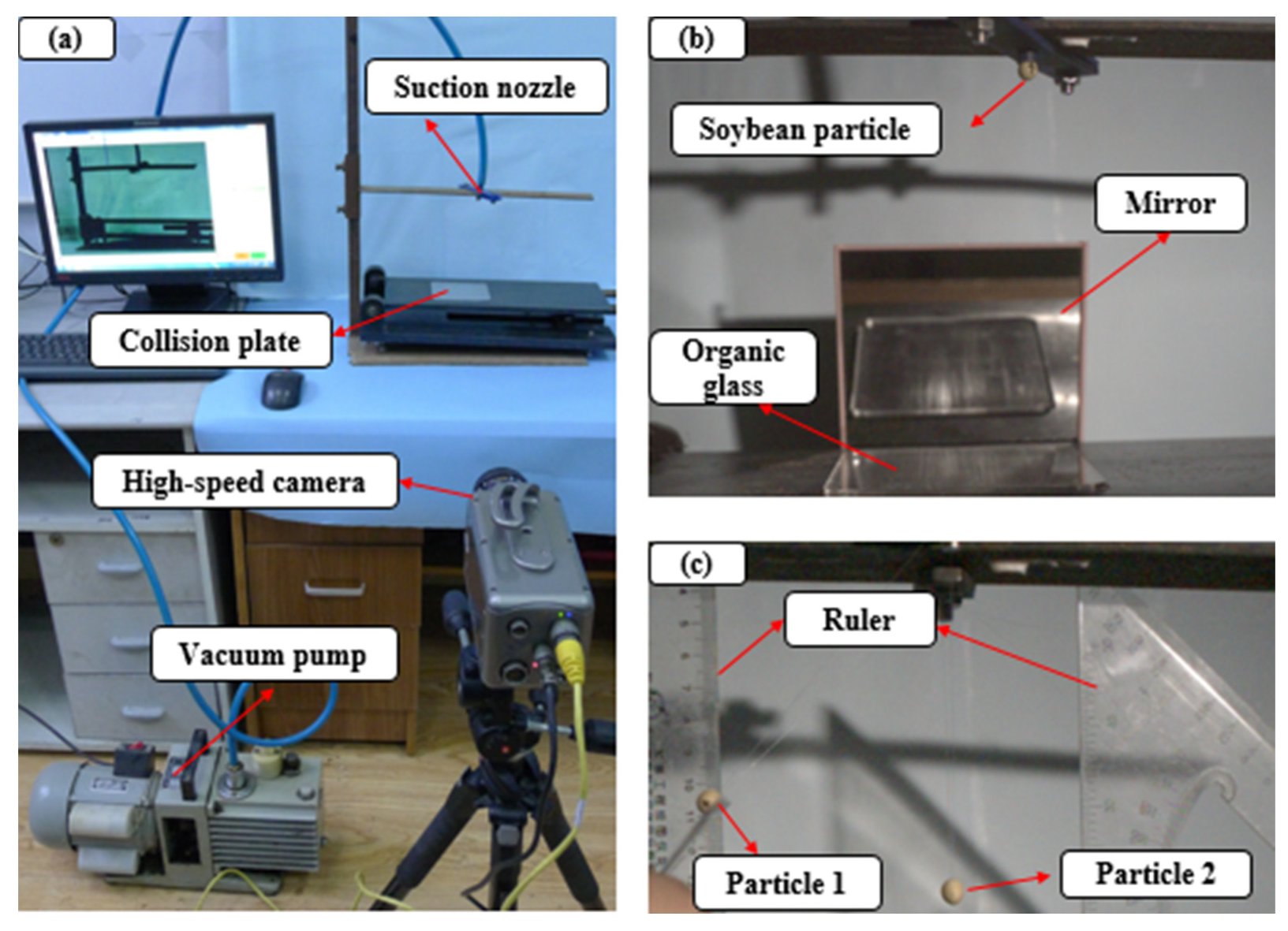
3.1. Test Analysis

3.1.1. “Self-Flow Screening” Test

As the soybean particle can be approximately ellipsoid, the circular-aperture sieve is selected to perform the “self-flow screening” test. The simulation is used to select the inclination angle and aperture size, see Figure 6a. EDEM [6] is chosen as the simulation software (EDEM2018, DEM Solutions, Edinburgh, UK, 2002) and the 13-ball model of J-17 is selected as the particle model. The parameters in EDEM simulation are listed in

Table 2. Parameters used in the simulation.

Parameters	Symbol	S-42			J-17			Z-39
		Soybean Seed	Organic Glass	Galvanized Steel	Soybean Seed	Organic Glass	Galvanized Steel	Soybean Seed	Organic Glass	Galvanized Steel
Density, kg/m3	ρ	1257	1800	7850	1213	1800	7850	1192	1800	7850
Poisson ratio	ν	0.4	0.25	0.3	0.4	0.25	0.3	0.4	0.25	0.3
Modulus of elasticity, Pa	E	7.6 × 108	1.3 × 108	7.9 × 1011	6.1 × 108	1.3 × 108	7.9 × 1011	2.6 × 108	1.3 × 108	7.9 × 1011
Coefficient of static friction	μ	0.2	0.228	0.259	0.2	0.228	0.247	0.2	0.235	0.277
Coefficient of rolling friction	μr	0.02	0.05	0.02	0.03	0.04	0.05	0.03	0.04	0.04
Coefficient of restitution	$e$	0.627	0.542	0.647	0.562	0.642	0.715	0.607	0.705	0.726
Normal stiffness, N/m	$k_{t,n}$	2219	759	1.1 × 106	1655	709	1.0 × 106	751	751	1.1 × 106
Tangential stiffness, N/m	$k_{t,t}$	792	303	4.2 × 105	591	283	4.0 × 105	268	300	4.2 × 105
Normal damping coefficient, kg/s	${\eta }_{t,n}$	0.185	0.123	4.02	0.185	0.08	2.66	0.105	0.071	2.84
Tangential damping coefficient, kg/s	${\eta }_{t,t}$	0.061	0.041	1.331	0.06	0.026	0.880	0.034	0.024	0.940

.

J-17 is taken as the example. When the aperture size is large enough (9 mm), the simulated percentages passing for the inclination angle ranging from 5° to 11°. When the inclination angle is larger than 10°, the percentage passing of simulation tends to be stable, see Figure 7a. Thus, the inclination angle of the “self-flow screening” device for J-17 is chosen as 11° in this paper. The percentages passing of the simulation for the aperture diameter changing from 6.6 to 8.2 mm. When the aperture size is larger than 7.6 mm, the simulated percentage passing becomes stable, see Figure 7b. Therefore, the aperture diameter of the “self-flow screening” device for J-17 is chosen as 7.8 mm in this paper. By the same way, the inclination angle and aperture diameter of the “self-flow screening” device for S-42 are determined as 7° and 8.0 mm; the inclination angle and aperture diameter of the “self-flow screening” device for Z-39 are determined as 15° and 8.2 mm.

The procedure of the “self-flow screening” test is as follows: A total of 1000 soybean particles are first uniformly dropped into the charging box. When all the particles have settled down, the plugboard is then pulled out. Under the action of gravity, the particles flow down along the surface of the sieve. After the moving of particles is finished, particles are distributed on the surface of the sieve or in the receiving box. The receiving box consists of four zones, named as 1, 2, 3, and 4. The zone above the sieve-deck is named as 5, see Figure 6b. After the “self-flow screening” test is finished, the number of soybean particles in these five zones are counted, and then the percentage of passing is calculated. The “self-flow screening” test is repeated five times for S-42, J-17, and Z-39, respectively.

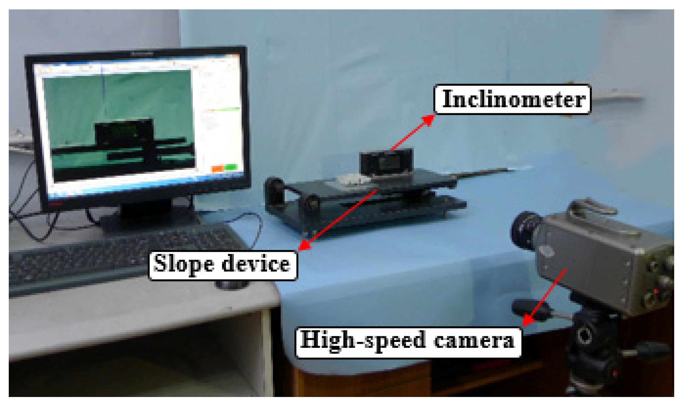
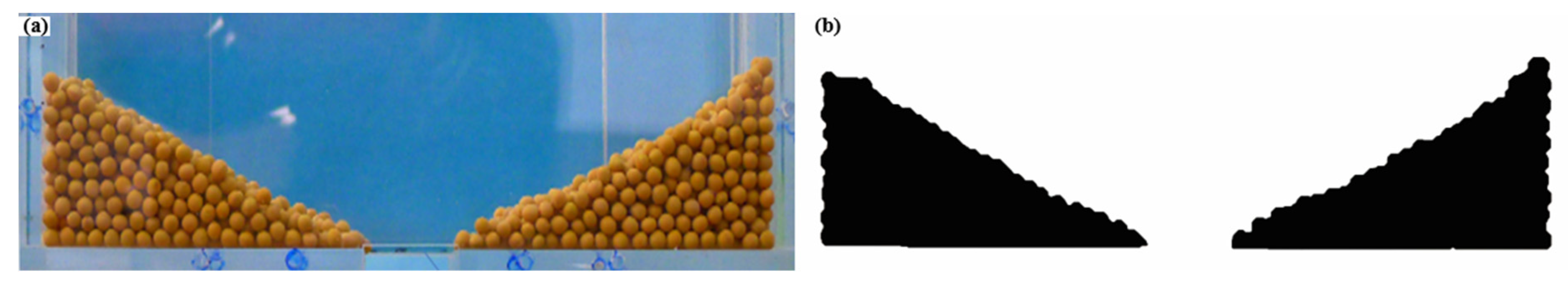
3.1.2. “Piling Angle” Test

Figure 8 illustrates the structure and size of the piling box. The length and width of the piling box and the amount of the soybean particles are determined by simulation. EDEM is used as the simulation software. The 13-ball model of J-17 is employed as the particle model. The parameters in EDEM simulation are listed in Table 2.

The choosing of the length of the piling box is taken as the example. When the width of the piling box is 80 mm and the amount of soybean particles is enough, the variations of the piling angle are simulated for different lengths of the piling box (140, 160, 180, 200, 220, 240, 260 mm), see Figure 9a. When the length of the piling box is no smaller than 180 mm, the piling angle trends to be stable. Thus, the length of the piling box is chosen as 220 mm. When the length is 220 mm, the width of the piling box and the amount of soybean particles are determined in the same way as 48 mm and 4000, respectively, as depicted in Figure 9b,c.

The procedure of the “piling angle” test is as follows: A total of 4000 soybean particles are first put into the charging box. When all the particles have settled down, the plugboard is then pulled out. Simultaneously, the particles outflow from the charging box from the opening on the bottom, and the piling angle is formed in the charging box, see Figure 10a. The binarization of the photo of the piling angle is performed to get a fitting line and; therefore, the piling angle can be measured precisely, see Figure 10b,c. The “piling angle” test is repeated five times for S-42, J-17, and Z-39, respectively.

3.2. Simulation Analysis

3.2.1. Selection of the Simulation Parameters

The simulation software EDEM and DEMSLab (free version, Zhejiang University, Zhe Jiang, China) [16] are employed to simulate the movement of particle models established by the multi-ball approach and the ellipsoidal equation approach, respectively.

These two software are developed based on the discrete element method, mainly used for discrete element simulation.

The simulation parameters used in the two software are the same. The moisture contents of soybean particles for S-42, J-17, and Z-39 are 10.31%, 8.08%, and 11.1%, respectively. The parameters measured by experiment [14], as listed in Table 2, are close to those recommended by Horabik [17]. The value of Poisson’s ratio is accordance with the ASAE Standards [18,19]. The particle density is measured by the pycnometer approach. The Young’s modulus of soybean grains is determined by universal testing machine, see Figure 11. The force–displacement curves are obtained by compressing a soybean particle along the directions on which its length, width, and thickness lay, respectively. The Young’s modulus is calculated by averaging the results along the above three directions. The test is repeated five times for each variety of soybean particles.

The static coefficients of friction are measured by the inclined plane approach, see Figure 12. When the test begins, the free end of the inclined plate is lifted at a constant speed, the reading of the digital inclinometer is captured by a high-speed camera when the soybean particle starts to slide. The static coefficient of friction is then calculated as the tangent of the angle. The test is repeated five times for each variety of soybean particles.

The coefficients of restitution are obtained by the dropping test and the pendulum test, respectively, see Figure 13a–c. A soybean grain is first suck beneath the suction nozzle. When the vacuum pump (Figure 13a) is turned off, the soybean grain falls with no initial velocity. After the soybean particle contacts with the boundary directly, the soybean particle rebounds vertically. The whole process is recorded by a high-speed camera, and; therefore, the coefficient of restitution between a particle and a boundary is calculated (Figure 13b). Two soybean particles are connected by two wires of equal-length, respectively. One particle is raised up to a certain height (Figure 13c), and then it is released to contact with another particle directly. The whole process is recorded by a high-speed camera and thus the coefficient of restitution between two particles is calculated.

The density, Young’s modulus, and Poisson’s ratio of boundary material are the same as Xu’s simulations [6]. The coefficients of rolling friction are determined by means of calibration. The DEMSLab simulation parameters, such as the normal and tangential stiffness between particles and between the particle and the boundary, as well as the coefficients of normal and tangential damping between particles and between the particle and the boundary, are listed in Table 2 [14]. The linear spring model is used in both software.

3.2.2. Generation of Assembly of Particles

In this paper, 200 grains were first selected for each variety of soybean seeds. The average tri-axial sizes were then calculated. It is known that the tri-axial sizes obey normal distribution by the comprehensive analysis of the distribution of them. For the generation of an assembly of particles in the simulations of “self-flow screening” or “piling” processes, the particle model of a single soybean seed first needs to be built. In EDEM software, the multi-model of one single particle was obtained by the input of the coordinates and radii of each sub-balls in the particle model. In DEMSLab software, the ellipsoidal model of one single particle was built by the input of the averaged tri-axial sizes. Subsequently, the particle assembly was generated according to the normal distribution. This can guarantee that the particle assembly generated in EDEM is consistent with that generated in DEMSLab. The above process is the modelling of particle assembly.

3.2.3. Simulation Setup

(1)

“Self-flow screening” simulation

The EDEM and DEMSLab are employed to perform the simulations of the “self-flow screening” for five-, nine-, and 13-ball models and the multi-ball models other researchers established as well as the ellipsoidal equation model. The parameters used in the simulations are listed in Table 2. Firstly, the particle factory create 1000 particles, and then they fall into the charging box. After all the particles are stable in the charging box, the plugboard moves upwards perpendicular to the sieve deck. The particles move down along the sieve deck. When the movement of particles is finished, the particles stay either in the receiving box beneath the sieve deck or on the sieve deck. The numbers of particles in corresponding zones are counted.

(2)

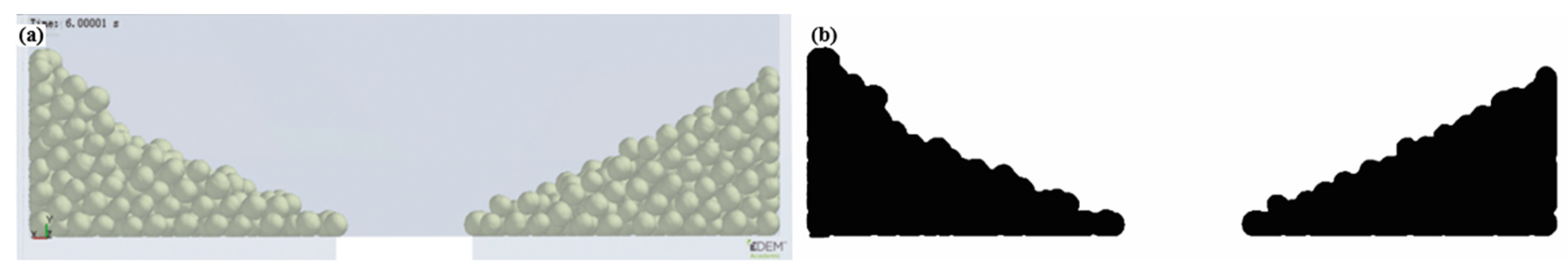
“Piling angle” simulation

The EDEM and DEMSLab are employed to conduct the simulations of the “piling angle”. The simulation parameters are listed in Table 2. First of all, the particle factory creates 4000 particles, after all the particles are settled down, the plugboard moves backwards, and then particles outflow from the charging box. When the movement of particles is finished, the filling angles are formed on two sides of the charging box. The piling angles are measured through image processing.

3.3. Result Analysis

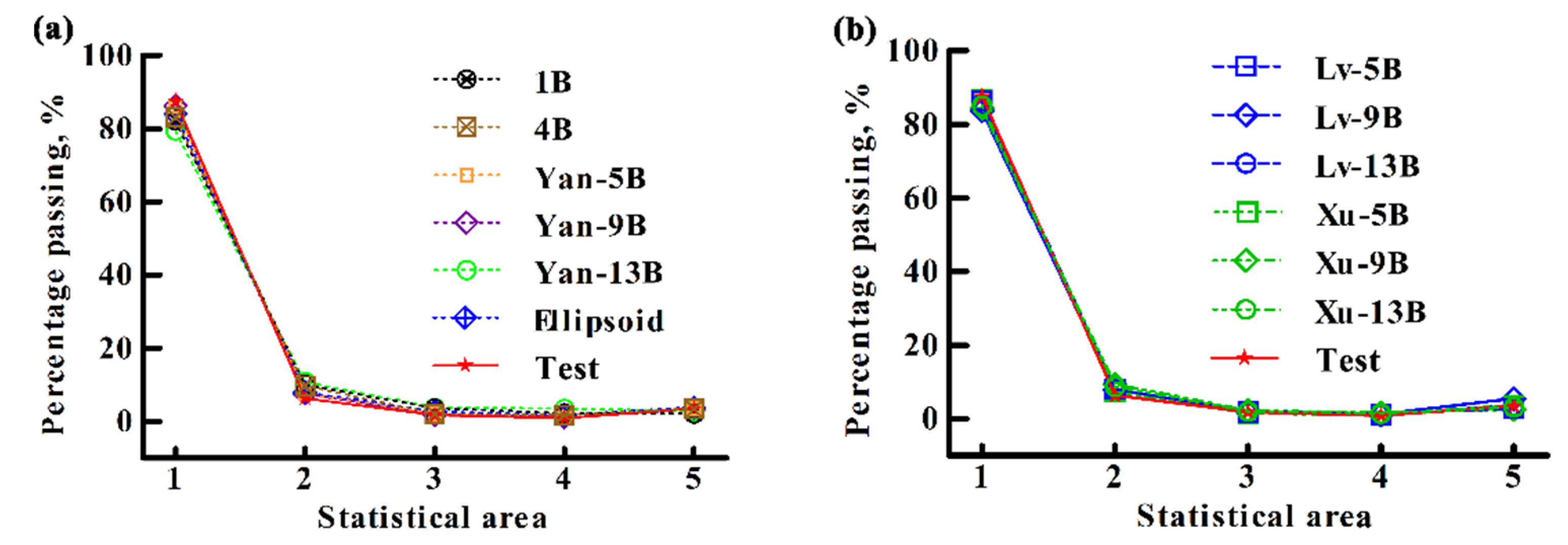
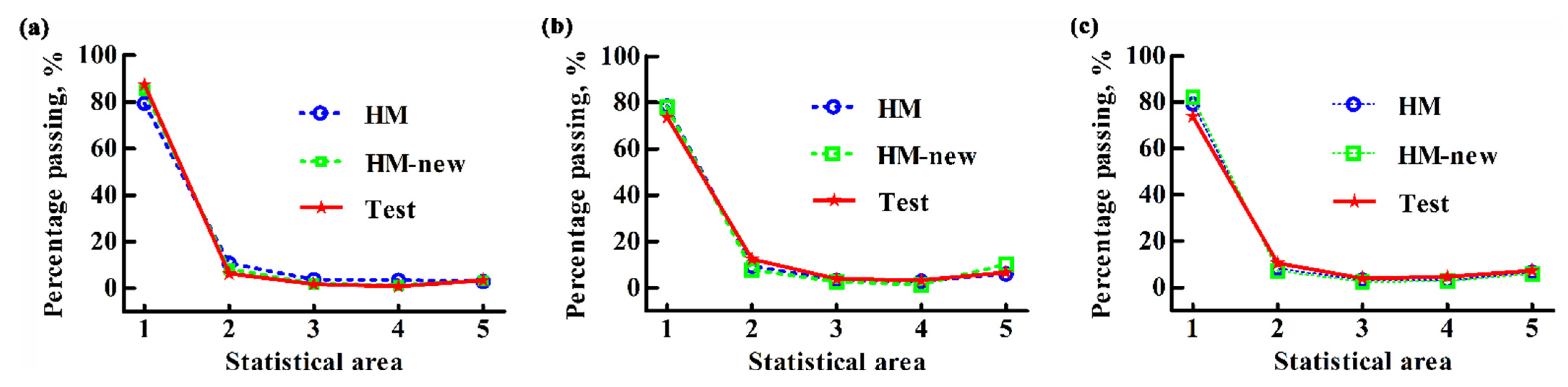
3.3.1. Result Analysis of the “Self-Flow Screening” Test

Figure 14a–c is the test photo, EDEM simulation snapshot, and DEMSLab simulation snapshot of the “self-flow screening”, respectively.

Figure 15, Figure 16 and Figure 17 depict the test results and the simulation results of percentage in terms of the amount of soybean particles for different statistical areas in the “self-flow screening”. It shows that the number of particles has the largest value in the No. 1 statistical area, and the amounts of particles in other statistical zones are relatively small. For the S-42 (sphericity 94.78%), the simulation results of all models are close to those obtained testy, see Figure 15a,b. For the J-17 (sphericity 86.86%), see Figure 16a,b, the simulation results of the 1B, 4B, Yan-9B, Yan-13B, Ellipsoid, and Xu-9B models are converged to the test results. For the Yan-5B, Xu-5B, Xu-13B, Lv-5B, Lv-9B, and Lv-13B models, their simulation results in the No. 1 statistical area are smaller than the test results, and their simulation results in the No. 5 statistical area are larger than the test results. These largely differ from the test data. For the Z-39 (sphericity 80.6%), see Figure 17a,b, the simulation results of the 4B-, Yan-9B, Yan-13B, Ellipsoid, and Xu-9B models are converged to the test results. For the 1B, Yan-5B, Xu-5B, Xu-13B, Lv-5B, Lv-9B, and Lv-13B models, their simulation results in the No. 1 statistical area are lower than the test results, and their simulation results in the No. 5 statistical area are larger than the test results. These largely differ from the test results.

From the above analysis, it can be seen that the multi-ball approach and the ellipsoidal equation approach are appropriate to model soybean particles with high sphericity; when the sphericity of particles is low, the 4B, Yan-9B, Yan-13B, and Xu-9B models are more applicable.

Figure 18 depicts the simulation results and the test results in terms of the percentage passing in the “self-flow screening”. For the S-42, see Figure 18a, the simulation results of the 4B, Yan-5B, Yan-9B, Yan-13B, Lv-13B, Xu-5B, and Xu-13B models are all within the error band of the test results. The simulation results of the Lv-5B and Xu-9B models are close to the test results. The simulation results of 1B and Lv-9B differ largely from the test results, and their differences are 2.1% and 1.3%, respectively. For the J-17, see Figure 18b, the simulation results of the Yan-13B and Xu-9B models are within the error band of the test results. The simulation results of the 1B, 4B, Yan-9B, and Ellipsoid models are a slight departure from the error band of the test results, their differences are 3.34%, 2.27%, 1.93%, and 2.71%, respectively. The other models’ simulation results differ largely from the test results. For the Z-39, see Figure 18c, the simulation results of the Yan-13B model are within the error band of test results, and the simulation results of the Yan-9B, Xu-9B, 4B, and Ellipsoid models are close to the test results; their errors are 0.6%, 1.9%, 2.07% and 2.63%, respectively. The other models’ simulation results differ largely from the test results.

The above analysis further proves that, except for the 1B model, all the models are appropriate for the modelling of soybean particles with high sphericity (e.g., the S-42); and for those with low sphericity (such as, the J-17 and Z-39), the Yan-9B and Yan-13B models presented in this paper as well as the Xu-9B model are more applicable than other models.

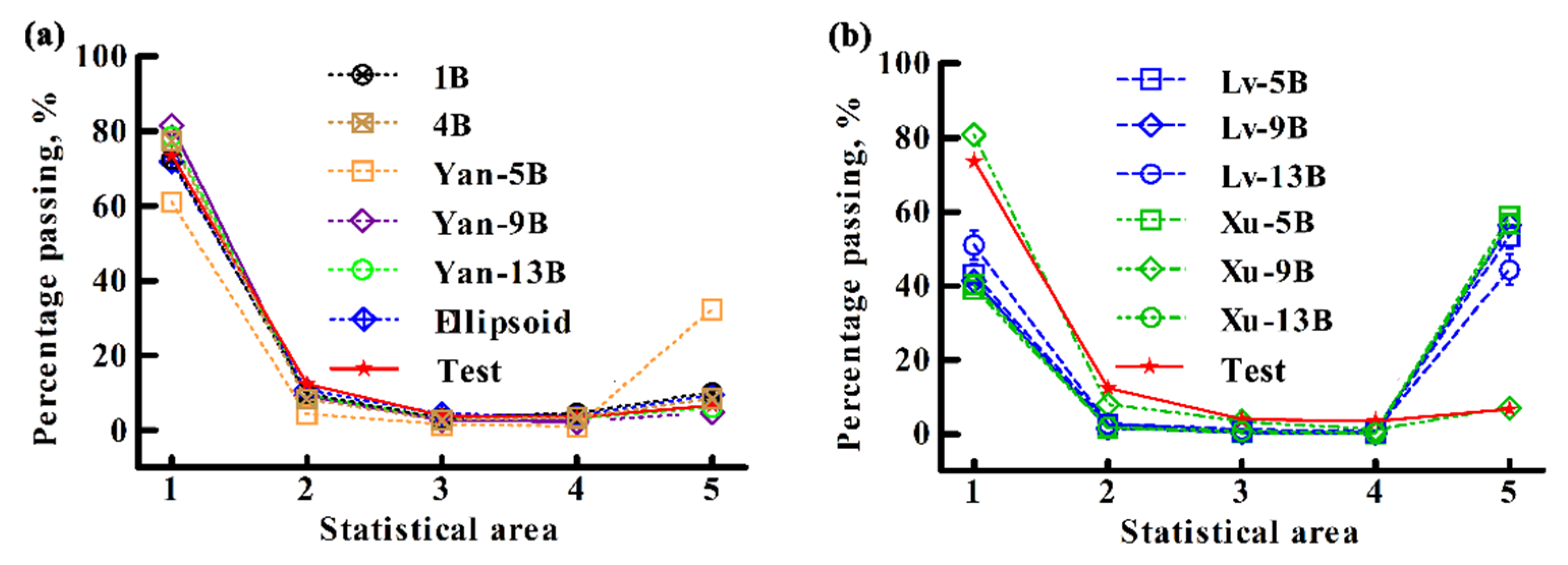
3.3.2. Result Analysis of the “Piling Angle” Test

Figure 19a,b shows the test photos of the “piling angle” test and their binarization images. Figure 20a,b shows the EDEM simulation snapshots of the “piling angle” test and their binarization images. Figure 21a,b shows the DEMSLab simulation snapshots of the “piling angle” test and their binarization images.

Figure 22a–c depicts the test results and the simulation results in terms of piling angle for different models of soybean particles from three varieties. For the soybean particles of S-42 (sphericity 94.78%), see Figure 22a, the simulation results of the Yan-5B, Yan-9B, Yan-13B, Xu-5B, and Xu-13B models are all within the error band of the test results. The simulation results of the 1B, 4B, Lv-9B, Lv-13B, Xu-9B, and Ellipsoid models deviate from the test results, and their errors are 6.86°, 1.49°, 1.49°, 1.62°, 1.19°, and 7.89°, respectively. For the soybean particles of J-17 (sphericity 86.86%), see Figure 22b, only the Yan-13B model’ simulation result is within the error band of the test results. The Yan-9B model’ simulation result slightly exceeds the test result, and its error is 0.49°. The other models’ simulation results largely deviate from the test results. For the soybean particle of Z-39 (sphericity 80.6%), see Figure 22c, except for the Yan-9B, Yan-13B, Lv-9B, and Lv-13B models which are within the error band of the test results, all the other models’ simulation results largely deviate from the test results.

It can be seen from the above analysis that the 1B, 4B, and Ellipsoid models are not suitable for the modelling of the “piling angle” test. There exists a big difference between the test results and the simulation results of the multi-ball models Lv and Xu presented, and the variations of the simulation results for soybean particles with different varieties are large. The multi-ball models presented in this paper are not only suitable for soybean particles with high sphericity, but also applicable to those with low sphericity, except for the Yan-5B model.

By the comprehensive comparisons of the simulation results with the test results in both the “piling angle” test and the “self-flow screening” test, it can be concluded that, compared with the 1B model, 4B model, and the multi-ball models Xu and Lv presented as well as the ellipsoid model, the multi-ball models presented in this paper are more appropriate for the modelling of soybean particles. For the soybean particles with high sphericity, the five-, nine-, and 13-ball models established in this paper are all applicable; for those with low sphericity, the five-ball model is not appropriate at all, but the nine- and 13-ball models are still appropriate. Therefore, the five-ball model (Yan-5B) is recommended for the modelling of soybean particles with high sphericity, the nine- and 13 ball models (Yan-9B and Yan-13B) are recommended for the modelling of soybean particles with low sphericity.

4. Influence of the Multiple Contacts

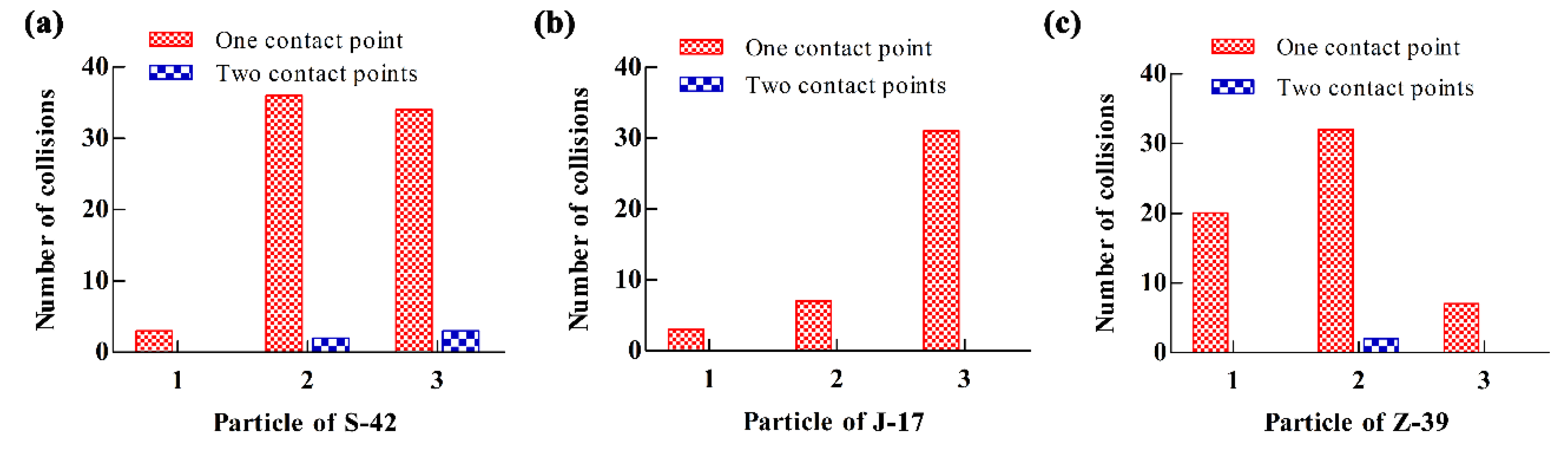
4.1. Simulation Analysis of the Multiple Contacts

The multiple contacts issue widely exists in the simulation of multi-ball models. When the EDEM software is used to simulate, the HM-new-restitution (short for HM-new) can be used to reduce the influence of the multiple contacts properly. Thus, the HM-new model is used to study the influence of the multiple contacts on the multi-ball models presented in this paper. The Hertz-Mindlin (no-slip) (short for HM) established-in model in EDEM is also used for the comparison with the HM-new model. The Yan-13B model is herein selected in the simulations.

Figure 23a is the comparison of the simulation results of both the HM model and the HM-new model with the test results in terms of the piling angle for soybean particles in three varieties. It can be seen from Figure 23a that there is no difference between the simulation results of the HM model and those of the HM-new model, and they are both close to the test results.

Figure 23b is the comparison of the simulation results of both the HM model and the HM-new model with the test results in terms of the percentage passing in the “self-flow screening” for soybean particles in three varieties. There is no discrepancy between the simulation results of the HM model and those of the HM-new model, and they are both close to the test results. Figure 24a–c presents the comparison of the simulation results of both the HM model and the HM-new model with the test results in terms of the percentages of grain number in different statistical areas for soybean particles in three varieties. It shows that the variations between the simulation results of the HM model and those of the HM-new model are small, and both of them converge to the test results.

By the comprehensive analysis, it can be known that the simulation results of the HM model are close to those of the HM-new model. This means that the multiple contacts has little impact on the movement of an assembly of multi-ball particles.

4.2. Reason Analysis

To investigate the reason why the multiple contacts has little impact on the simulation results, the movement of one soybean particle established by the 13-ball model flowing on the sieve-deck in the “self-flow screening” device was simulated. As the variation in sphericity of soybean particles from three varieties are large, three particles were set for each variety in the simulation. The numbers of contact points between the particle and the sieve-deck in a collision for each particle were counted by the EDEM analyst, see Figure 25a–c.

In the period when one single soybean particle moved along the sieve-deck, for the soybean particles of the S-42 (Figure 25a), the number of particle–deck collisions for the three particles is 78, where the number of collisions for one contact point is 73 and the number of collisions for two contact points is 5; for the soybean particles of the J-17 (Figure 25b), the number of particle–deck collisions for the three particles is 41, where all the number of contact point are one for each collision; for the soybean particles of Z-39 (Figure 25c), the number of particle–deck collisions for the three particles is 59, where the number of collisions for one contact point is 57, and the number of collisions for two contact point is 2. Overall, the collisions with one contact point are dominant, which account for 97.2%. The number of contact points is up to two. The amount of the collisions with two contact points is relatively small, and its proportion is only 2.8%. It can be shown from the above analysis that the number of contact points is not too many for each collision when the particle model established in this paper flowing on the surface of sieve and the multiple contacts has little impact on the movement of particles.

5. Conclusions

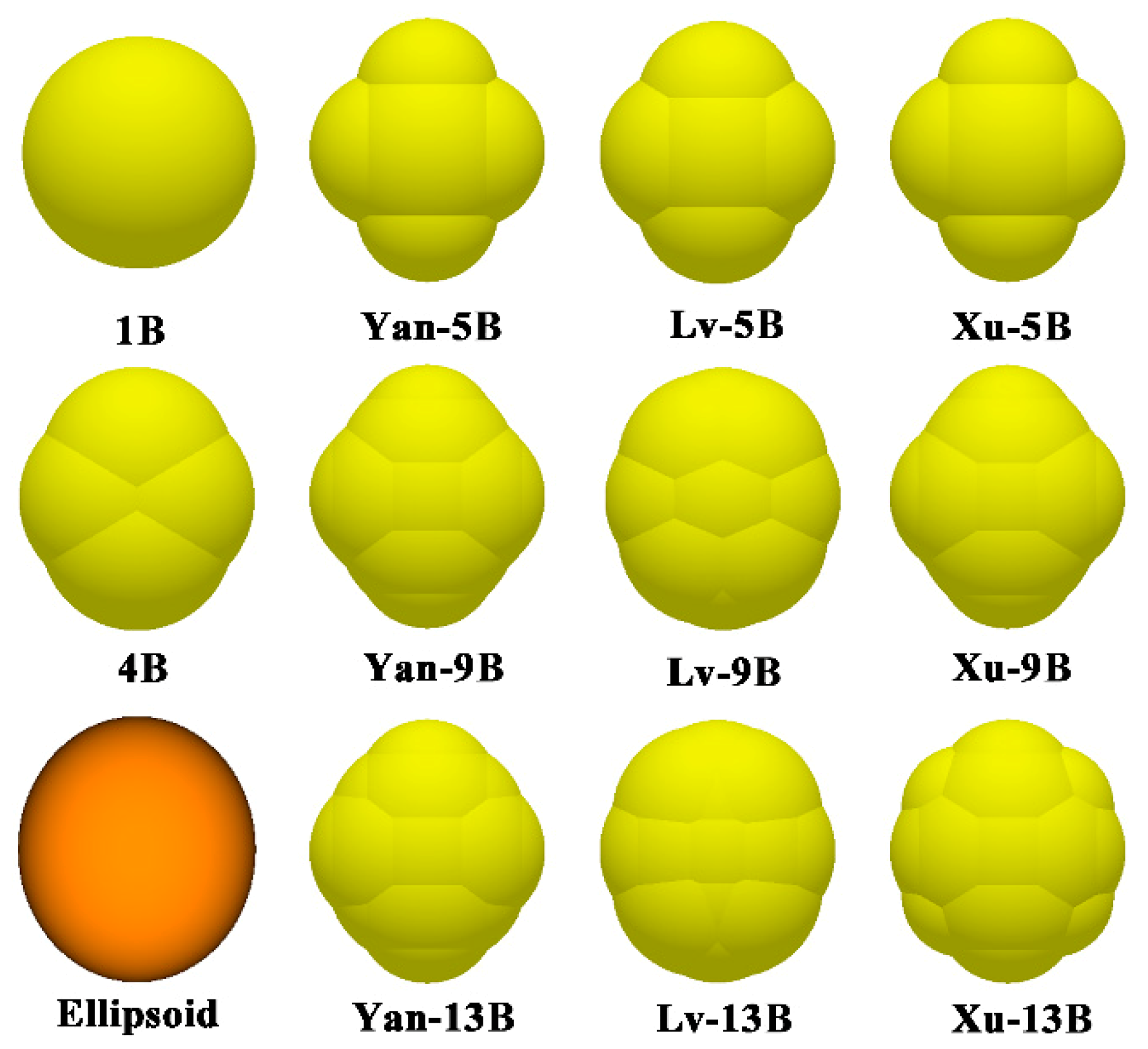
• A novel modelling approach for soybean particles presented in this paper is introduced, namely one single soybean particle modelled by five, nine, and 13 balls “gluing” together, respectively.
• The multi-ball models presented in this paper are compared with the ellipsoidal model, as well as the models other researchers (home and abroad) established by comparison between the simulation results and the test results, in terms of the “self-flow screening” and “piling angle” tests. It is shown that the modelling approach presented in this paper has stronger applicability than other approaches. For the soybean particle with high sphericity, the five-ball model is appropriate; for those with low sphericity, the nine- and 13-ball models are more applicable. Additionally, if the time cost is not considered, and the consistency between the simulation and the experiment is only concerned, the 13-ball model is the most recommended.
• The simulation results of the “piling angle” and “self-flow screening” using the HM-new model are basically the same as those employing the HM model and are close to the test results. This proves that the multiple contacts has little impact on the movement of particles modelled by the multi-ball approach.

References

1. Cundall, P.A.; Strack, O.L. A discrete numerical model for granular assemblies. Géotechnique 1979, 29, 47–65. [Google Scholar] [CrossRef]
2. Lu, Z.; Negi, S.C.; Jofriet, J.C. A numerical model for flow of granular materials in silos. Part 1: Model development. J. Agric. Eng. Res. 1997, 68, 223–229. [Google Scholar] [CrossRef]
3. Vu-Quoc, L.; Zhang, X.; Walton, O.R. A 3-D discrete-element method for dry granular flows of ellipsoidal particles. Comput. Methods Appl. Mech. Eng. 2000, 187, 483–528. [Google Scholar] [CrossRef]
4. Boac, J.M.; Casada, M.E.; Maghirang, R.G.; Harner, J.P. Material and interaction properties of selected grains and oilseeds for modeling discrete particles. Trans. ASABE 2010, 53, 1201–1216. [Google Scholar] [CrossRef] [Green Version]
5. Lv, F. Investigation of Physical and Mechanical Properties and Modelling Method for Soybean Grains. Available online: https://kns.cnki.net/KCMS/detail/detail.aspx?filename=1017160847.nh&dbname=CMFDTEMP (accessed on 10 January 2021).
6. Xu, T.; Yu, J.; Wang, Y. A modelling and verification approach for soybean seed particles using the discrete element method. Adv. Powder Technol. 2018, 29, 3274–3290. [Google Scholar] [CrossRef]
7. Lin, X.S.; Ng, T.T. Contact detection algorithms for 3-dimensional ellipsoids in discrete element modeling. Int. J. Numer. Anal. Methods Geomech. 1995, 19, 653–659. [Google Scholar] [CrossRef]
8. Ouadfel, H.; Rothenburg, L. An algorithm for detecting inter-ellipsoid contacts. Comput. Geotech. 1999, 24, 245–263. [Google Scholar] [CrossRef]
9. Saini, N.; Kleinstreuer, C. A new collision model for ellipsoidal particles in shear flow. J. Comput. Phys. 2019, 376, 1028–1050. [Google Scholar] [CrossRef]
10. Markauskas, D.; Kačianauskas, R.; Džiugys, A.; Navakas, R. Investigation of adequacy of multi-ball approximation of elliptical particles for DEM simulations. Granul. Matter 2010, 12, 107–123. [Google Scholar] [CrossRef]
11. Kodama, M.; Bharadwajb, R.; Curtisc, J.; Hancockb, B.; Wassgren, C. Force model considerations for glued-ball discrete element method simulations. Chem. Eng. Sci. 2009, 64, 3466–3475. [Google Scholar] [CrossRef]
12. Wang, X. A Multi-ball Based Modelling Method for Maize Grain Assemblies. Adv. Powder Technol. 2017, 28, 584–595. [Google Scholar] [CrossRef]
13. Kruggel-Emden, H.; Rickelt, S.; Wirtz, S.; Scherer, V. A study on the validity of the multi-ball discrete element method. Powder Technol. 2008, 188, 153–165. [Google Scholar] [CrossRef]
14. Yan, D.; Yu, J.; Wang, Y.; Zhou, L.; Yu, Y. A general modelling method for soybean seeds based on the discrete element method. Powder Technol. 2020, 372, 212–226. [Google Scholar] [CrossRef]
15. Boac, J.M.; Ambrose, R.K.; Casada, M.E.; Maghirang, R.G.; Maier, D.E. Applications of Discrete Element Method in Modeling of Grain Postharvest Operations. Food Eng. Rev. 2014, 6, 128–149. [Google Scholar] [CrossRef] [Green Version]
16. You, Y.; Zhao, Y. Discrete elementmodelling of ellipsoidal particles using super-ellipsoids and multi-balls: A comparative study. Powder Technol. 2018, 331, 179–191. [Google Scholar] [CrossRef]
17. Horabik, J.; Molenda, M. Parameters and contact models for DEM simulations of agricultural granular materials: A review. Biosyst. Eng. 2016, 147, 206–225. [Google Scholar] [CrossRef]
18. Coskun, M.B.; Yalçin, Ì.; Özarslan, C. Physical properties of sweet corn seed (Zea mays saccharata Sturt). J. Food Eng. 2006, 74, 523–528. [Google Scholar] [CrossRef]
19. USA, American Society of Agricultural Engineers. Compression Test of Food Materials of Convex Shape, ASAE Standards 2002: Standards Engineering Practices; American Society of Agricultural Engineers: St. Joseph, MI, USA, 2002; Volume 49, pp. 592–599. Available online: http://www.doc88.com/p-3347853614932.html (accessed on 10 January 2021).
Figure 1. Triaxial sizes of one single soybean particle under the space rectangular coordinate system.
Processes 09 00286 g001
Figure 2. Introduction to the multi-ball modelling approach for the (a) five-ball model, (b) nine-ball model, and (c) 13-ball model.
Processes 09 00286 g002
Figure 3. Comparison of models established by different approaches for one single soybean particle of S-42.
Processes 09 00286 g003
Figure 4. Comparison of models established by different approaches for one single soybean particle of J-17.
Processes 09 00286 g004
Figure 5. Comparison of models established by different approaches for one single soybean particle of Z-39.
Processes 09 00286 g005
Figure 6. (a) Device of the “self-flow screening” and (b) the statistical areas of the device.
Processes 09 00286 g006
Figure 7. For the soybean particle of J-17: (a) The relation between the percentage passing and the inclination angle, (b) the relation between the percentage passing and the aperture size.
Processes 09 00286 g007
Figure 8. Schematic diagram of the piling box.
Processes 09 00286 g008
Figure 9. Variations of the angle of piling with the (a) length and (b) width of the piling box and (c) the amount of particles in the “piling angle” simulations for J-17.
Processes 09 00286 g009
Figure 10. (a) Photo of the piling angles, (b) binarization image of the piling angles, and (c) the fitting line of the outline of the binarization image.
Processes 09 00286 g010
Figure 11. Machine used for the compression of soybean particle.
Processes 09 00286 g011
Figure 12. Device for the measurement of the coefficient of static friction.
Processes 09 00286 g012
Figure 13. (a) Device for the measurement of the coefficient of restitution and the photos for measuring: (b) The coefficient of restitution between the particle and the boundary and (c) the coefficient of restitution between two particles.
Processes 09 00286 g013
Figure 14. (a) Test photo, (b) EDEM software simulation snapshot, and (c) DEMSLab software simulation snapshot of the “self-flow screening”.
Processes 09 00286 g014
Figure 15. Comparisons of the simulated percentages passing with the test ones in different statistical areas in the “self-flow screening” of S-42 soybean particles for (a) the 1B, 4B, Yan-5B, Yan-9B, Yan-13B, and Ellipsoid models, as well as (b) the Lv-5B, Lv-9B, Lv-13B, Xu-5B, Xu-9B, and Xu-13B models.
Processes 09 00286 g015
Figure 16. Comparisons of the simulated percentages passing with the test ones in different statistical areas in the “self-flow screening” of J-17 soybean particles for (a) the 1B, 4B, Yan-5B, Yan-9B, Yan-13B, and Ellipsoid models, as well as (b) the Lv-5B, Lv-9B, Lv-13B, Xu-5B, Xu-9B, and Xu-13B models.
Processes 09 00286 g016
Figure 17. Comparisons of the simulated percentages passing with the test ones in different statistical areas in the “self-flow screening” of Z-39 soybean particles for (a) the 1B, 4B, Yan-5B, Yan-9B, Yan-13B, and Ellipsoid models, as well as (b) the Lv-5B, Lv-9B, Lv-13B, Xu-5B, Xu-9B, and Xu-13B models.
Processes 09 00286 g017
Figure 18. Comparisons between the test results and the simulation results of different models in terms of the percentage passing for soybean particles of (a) S-42, (b) J-17, and (c) Z-39.
Processes 09 00286 g018
Figure 19. (a) Test photo of the piling angles and (b) its binarization image.
Processes 09 00286 g019
Figure 20. (a) EDEM simulation snapshot of the piling angles and (b) its binarization image using the 13-ball model.
Processes 09 00286 g020
Figure 21. (a) DEMSLab simulation snapshot of the piling angles and (b) its binarization image.
Processes 09 00286 g021
Figure 22. Comparisons between the test results and the simulation results of different models in terms of the piling angle for soybean particles of (a) S-42, (b) J-17, and (c) Z-39.
Processes 09 00286 g022
Figure 23. Comparisons of the test results with the simulation results using the Hertz-Mindlin (no-slip) (HM) and HM-new-restitution (HM-new) models for the simulations of (a) “piling angle” and (b) “self-flow screening”.
Processes 09 00286 g023
Figure 24. Comparisons between the simulation results and the test results of the percentage of particle numbers in different statistical areas for soybean particles of (a) S-42, (b) J-17, and (c) Z-39.
Processes 09 00286 g024
Figure 25. The number of particle–deck collisions for single soybean particles of (a) SN42, (b) JD17, and (c) Z-39.
Processes 09 00286 g025