1. Introduction
The production of butadiene rubber (BR) is an orientated polymerization process with butadiene as the monomer [
1]. BR ranks second in production among all kinds of rubber product in the world, only behind styrene butadiene rubber. It has the advantages of good elasticity, strong wear resistance, and low temperature resistance. Due to its excellent properties, BR has been extensively applied in the production of impact-resistant plastics, tires, tapes, hoses, rubber shoes, and other rubber products [
2]. Therefore, it is of great significance to ensure the safe and stable production of BR. In practice, the internal leakage of the heat exchanger network has always existed in the BR industry due to the deterioration of equipment. It is estimated that 10% of all corrosion damage in industrial systems results in leakage. However, internal leakage is usually hard to detect, e.g., 6.5 tons of liquid chlorine leaked unknowingly from a heat exchanger at Honeywell’s refrigerant production facility, leading to an emergency evacuation of the entire facility [
3]. Pressure difference is generally one of the main causes of internal leakage [
4]. The ionic components in the leakage flow may cause reduction reactions between water and the cathodic metallization and produce hydrogen gas and hydroxide ions [
5]. Consequently, internal leakage caused by pressure difference and corrosion can lead to adverse safety accidents and environmental impacts. Early warning and risk assessment are absolutely necessary for avoiding such leakage accidents.
In some emergency evacuation cases, the improper dissemination of evacuation warnings is the main cause of casualties [
6]. The cause analysis of major accidents shows that some accidents could have been avoided if appropriate preventive measures were put in place [
7]. Nevertheless, many early warning studies are difficult to provide a reliable description of emergency operations and further related preventive measures [
8]. In addition, the results of risk analysis are not comprehensive, so the accuracy and pertinence of monitoring and early warning are difficult to guarantee. Therefore, early warning methods need to be improved. Deep learning is considered as one of the most promising artificial intelligence technologies. It has attracted more and more research attention in recent years as early warning and data prediction using deep learning have great implication in the safety analysis of chemical processes. Based on deep learning, a generative adversarial networks-spearman’s rank correlation coefficient-deep belief networks (GAN-SRCC-DBN) method was proposed for the identification of abnormal conditions in chemical processes [
9]. However, most methods are limited to statistical methods and unable to capture the dynamic changes in the data deeply. Bayesian network has been widely used in the field of probabilistic safety analysis, but it ignores the time variable and is incapable of reflecting the evolution of the system variables over time [
10]. Another drawback of traditional neural networks is their inability to interpret time series based on specific context. Early attempts to solve this problem were Recurrent Neural Networks (RNN) based on the feedback method [
11]. However, it frequently leads to a gradient disappearance problem in certain applications. Long short-term memory (LSTM) is capable of alleviating these problems as a variant of RNN [
12]. LSTM was first proposed by Sepp Hochreiter and Jurgen Schmidhuber [
13]. It can maintain memory in their cellular state to figure out sequence and time problems without losing gradients that affect their performance. Its greatest strength consists in that it can learn the time variable introduced by dynamic simulation platforms to predict changes of risk variables over time. Hence, LSTM can be utilized to study the underlying mechanism in the model; then, it can be used to obtain quantitative results in disturbed conditions.
Dynamic simulation plays a significant role in process control strategy design, validation, and safety analysis. It introduces a time variable that reflects transient changes into the process when the system is disturbed. Therefore, it is widely used in chemical processes as the major tool for system safety analysis. For example, a novel DYN-SIL method combining dynamic simulation with the safety integrity level (SIL) was put forward to analyze the risk of the fluid catalytic cracking (FCC) fractionating system [
14]. Risk analysis and risk matrices combining dynamic simulation were presented to determine consequences and quantify severity [
15]. A semi-batch production of nitrile from fatty acid and ammonia was simulated using dynamic simulation to reduce batch cycle time [
16]. Dynamic simulation was used to formulate a suitable model for evaluating the overall dynamic characteristics of complex thermal recovery steam cycles [
17]. In general, dynamic simulation can be used to investigate the impact of variable fluctuations on safety response time when the variables reach the critical limit. So, the internal leakage within the heat exchanger network is studied in this paper utilizing dynamic simulation.
In recent years, a large number of safety accidents occurred in the chemical industry, resulting in a large number of deaths. Risk assessment is an essential requirement to ensure the safe design and operation of processes [
18]. Along with the increasing public appeal and strict government management, substantial sophisticated safety assessment methods and their improved methods have been widely employed in the past decade [
19]. Especially, SIL and hazard and operability analysis (HAZOP) are two of the most commonly used methods. However, those traditional methods cannot measure risk with high credibility [
20]. In order to address this problem, quantitative risk assessment (QRA) has attracted extensive attention from experts and scholars. QRA has been widely applied in various industries, including the nuclear industry, oil and gas industry, and steel industry [
21]. For example, a new QRA method integrated with dynamic simulation and accident simulation was proposed to discover inherent risks that are undetectable by conventional risk analysis methods based on steady-state conditions [
22,
23]. A risk-based accident model was used to conduct QRA and find the potential explosion risk for leakage failure of a submarine pipeline [
24,
25]. Dynamic variables were added to QRA to improve the operational performance analysis of chemical processes [
26]. Therefore, in this paper, QRA was employed to conduct the safety assessment of the heat exchanger network and obtain the quantitative ranges and destructive power of potential hazards caused by the internal leakage.
This paper realizes the early warning and risk assessment by combining DYN, LSTM, and QRA with regard to internal leakage of the heat exchanger network in the butadiene rubber polymerization unit. First, an internal leakage mechanism model of heat exchanger is built utilizing dynamic simulation. Based on this model, LSTM is trained to predict risk variables for constructing an early warning model. Finally, the ranges and destructive power of potential hazards are obtained using the QRA approach followed by the quantitative safety measures recommended. The remainder of this paper is arranged as follows.
Section 2 describes the BR process and dynamic simulations.
Section 3,
Section 4 and
Section 5 illustrates the heat exchanger network simulation, the early warning modeling, and risk assessment processes, respectively. Some important results are given in the final conclusion section.
2. Description of BR Process and DYN-EW-QRA Method
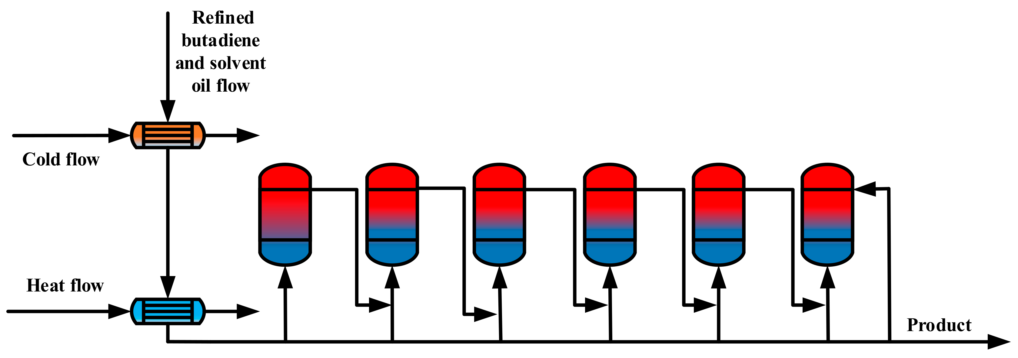
The BR production process consists of nine units: metering, polymerization, rubber tank, coagulation, rubber washing and drying, briquetting, packaging, solvent recovery, and waste gas treatment. Among them, the polymerization unit is the major research object. The glue generated by the polymerization reaction leaves from the top of the first reactor; then, it enters the bottom of the second reactor and other reactors in series. The jacket of each polymerization reactor is filled with frozen brine at −3 to −7 °C to adjust the reaction temperature. The schematic diagram of the polymerization unit in the BR process is shown in
Figure 1.
The internal leakage of the heat exchanger network in the feed section of the polymerization unit is studied in this internal leakage work. The main causes of heat exchanger internal leakage are the pressure difference and the corrosion phenomenon. In this heat exchanger network, a large pressure difference between the matter flow and the circulating water exists all the time. The circulating water system uses salt water, while the matter flow contains toxic, explosive, and flammable dangerous substances. Once this matter enters the circulating water, organic matters will become the nutrient of the microorganism, accelerating the reproduction of microorganisms and further aggravating the corrosion of the heat exchanger network. As a result, heat exchangers are susceptible to corrosion. Therefore, according to distributed control system (DCS) data, the heat exchanger with the largest pressure difference is selected for leakage case simulation.
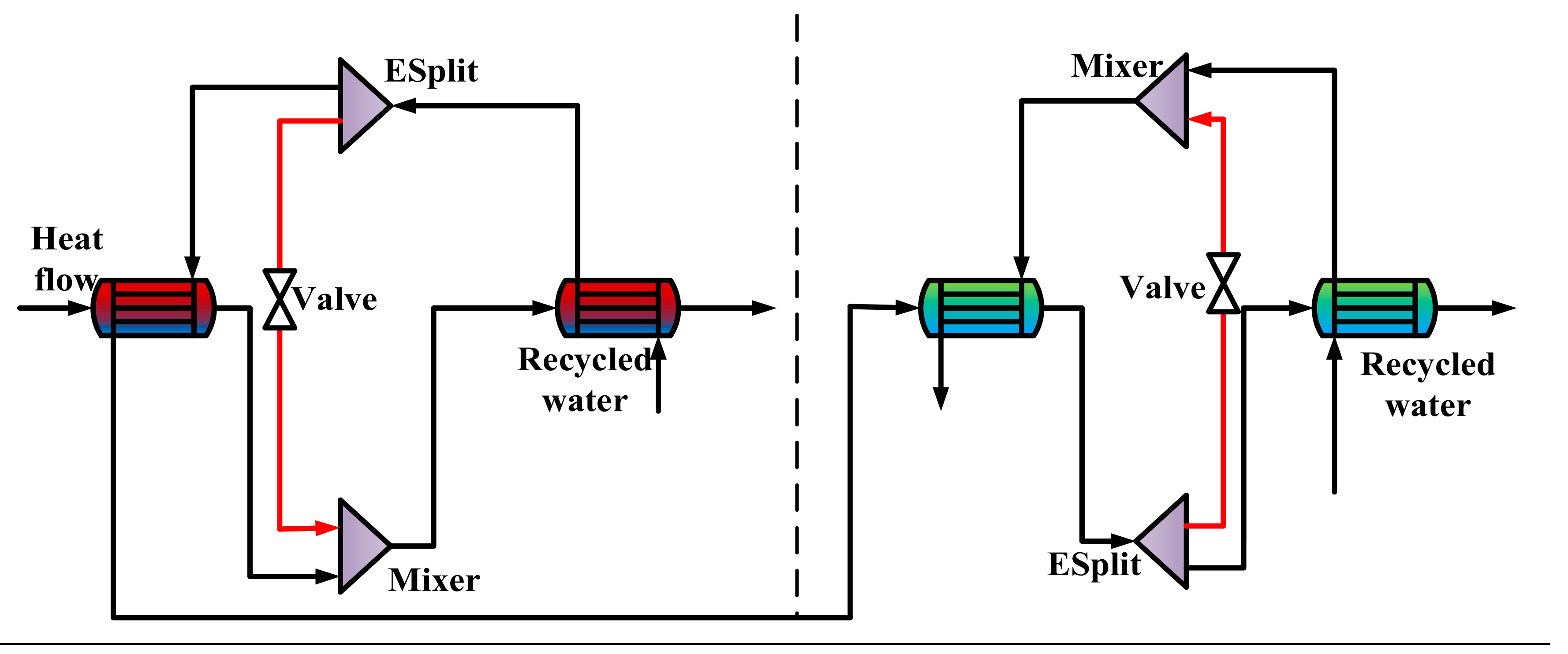
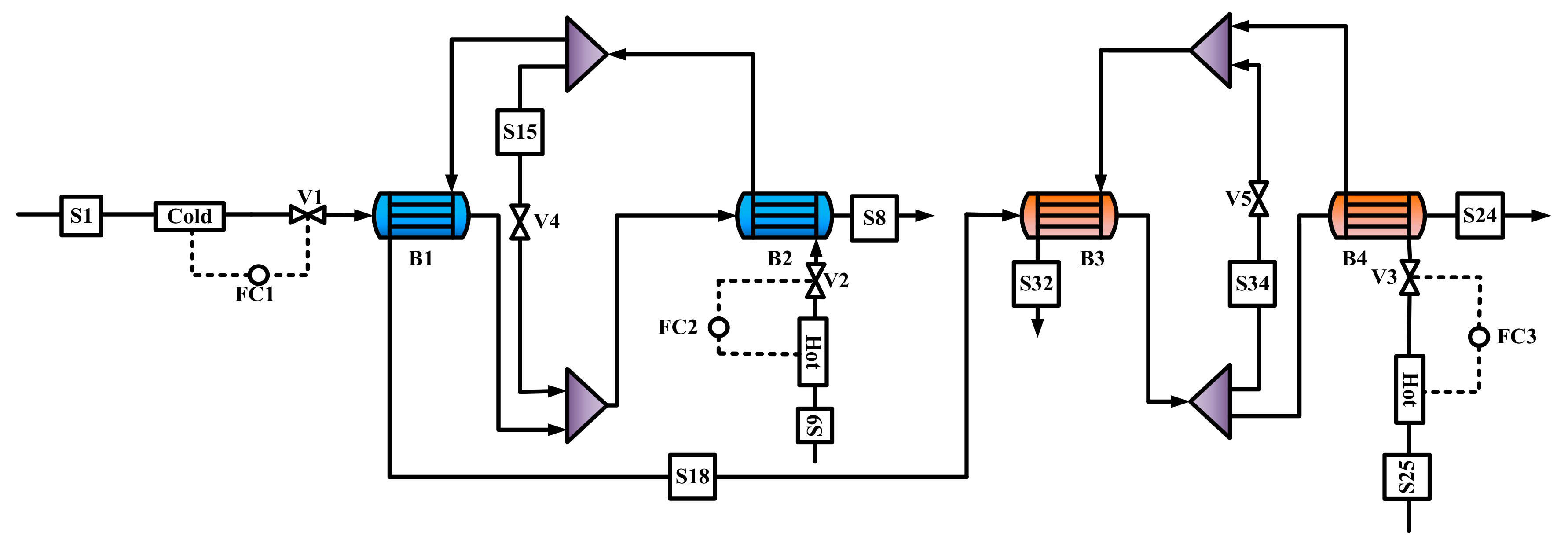
Due to the limitation of software functions, it is impossible to simulate the internal leakage of a single heat exchanger in detail and obtain the dynamic datasets of variables directly. As a consequence, we propose an internal leakage mechanism model, in which the leakage point of each heat exchanger is assumed to be one, and the internal leakage of each heat exchanger is simulated with two heat exchangers by adding mixers and splitters. The quantity of internal leakage is represented by the flow rate from the splitters, which is marked with the red line, as shown in
Figure 2.
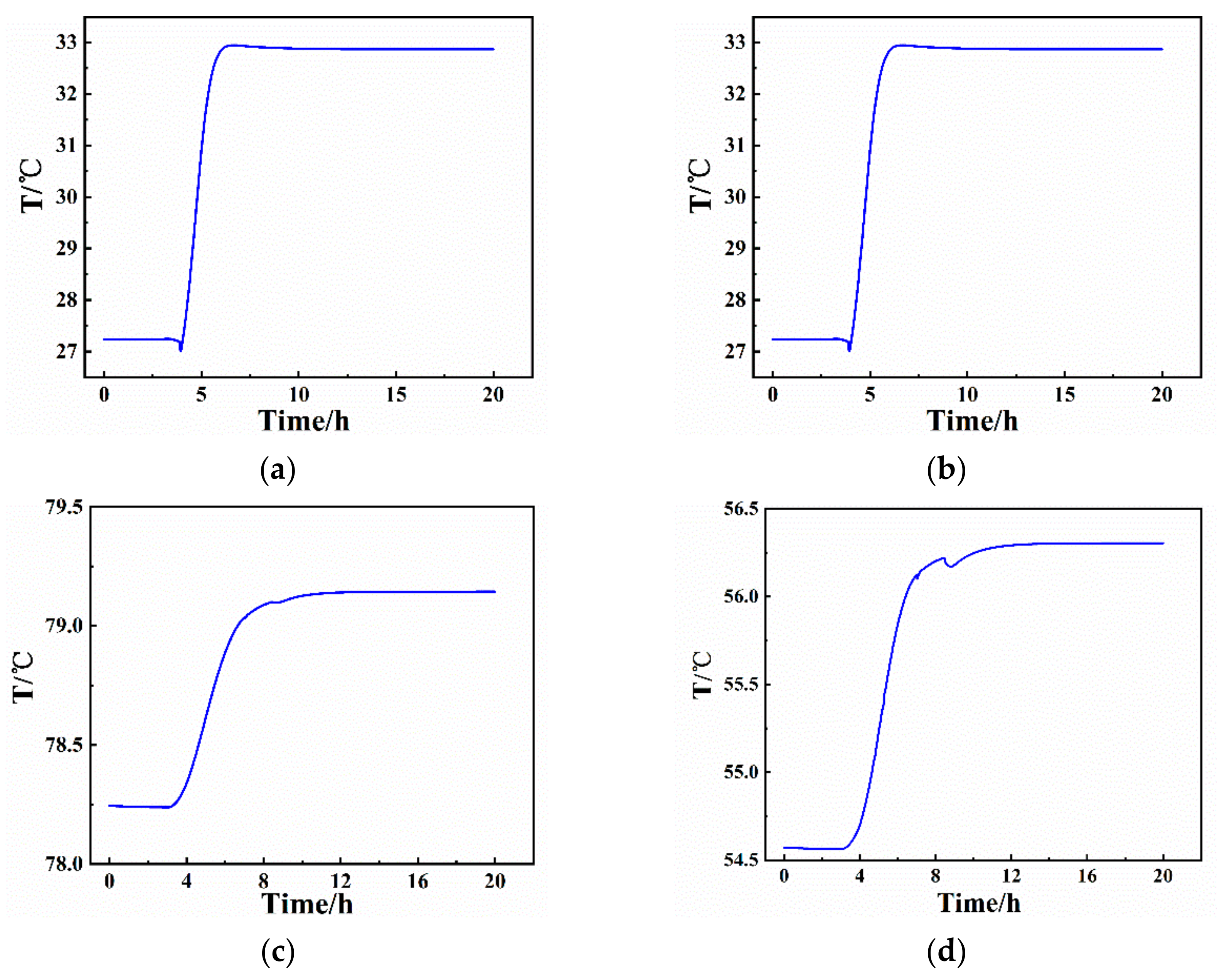
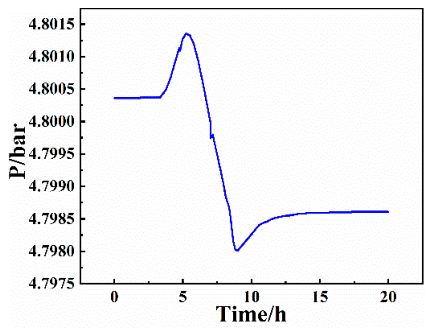
During BR production, the refined butadiene from the butadiene workshop is preheated, and it finally leaves the polymerization unit from the bottom of the last kettle. In
Figure 2, in order to simulate the matter leakage from the high-pressure side to the low-pressure side, the flow rate is changed by adjusting the parameters of splitters. In dynamic simulation, the flow can be adjusted by changing the valve opening. By adjusting the leakage rate from 0 to 20%, the corresponding temperature, pressure, flow rate, and other process data can be obtained.
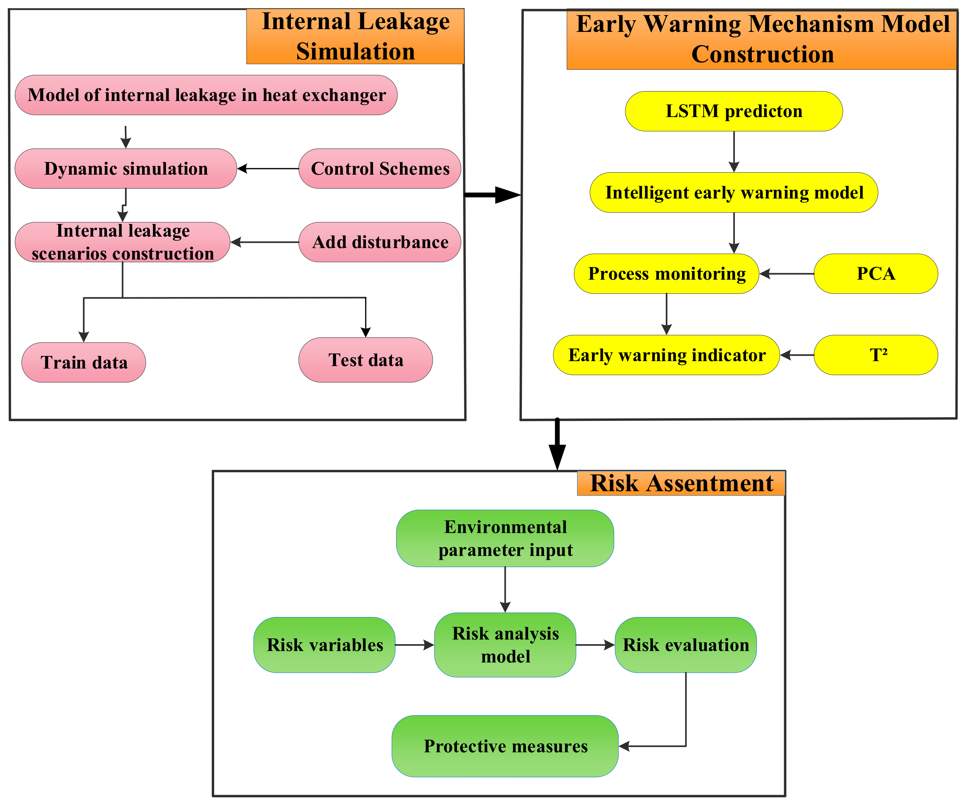
For the BR process, the DYN-EW-QRA method consists of three parts: (1) internal leakage simulation; (2) early warning mechanism model construction; and (3) risk assessment. Its framework is shown in
Figure 3.
The steady-state simulation is carried out to build a mechanism model based on the industrial parameters of the process. Then, the dynamic simulation is conducted based on the steady-state simulation, in which a control scheme is established to ensure the normal operation. Since the dynamic simulation takes into account the cumulative terms in the balance equation, the pressure magnitude of each module such as valves and mixers with retention capability will be adjusted. It also simulates leakage by adding disturbance to obtain time series process data. The VBA and ASM language (ASM dedicated to Aspen software) are used to simulate different internal leakage disturbance scenarios.
In the early warning stage, the normalized dynamic data are divided into a training set and a test set to carry out network prediction. LSTM is used to deeply analyze the influence of disturbance variables on the process. In order to obtain the optimal prediction results, the network hyper parameters need to be adjusted by the orthogonal parameter method. In the safety analysis stage, the range and destructive power of vapor cloud explosion hazards such as jet fire, flash fire, and explosive overpressure are calculated through the risk model with environmental parameters and variables.
4. Early Warning Model Construction
4.1. Model Construction and Optimization of LSTM
The dynamic dataset is obtained by simulating five internal leakage scenarios. For LSTM modeling, we simulate multiple disturbances as the training set and a single disturbance as a test set under the same conditions to verify the predictive result of the network. Furthermore, each set of 2000 continuous time samples is fed into the LSTM input gate in batches, constituting 22 sets in total. The training set and test set include 2000 and 4000 samples, respectively.
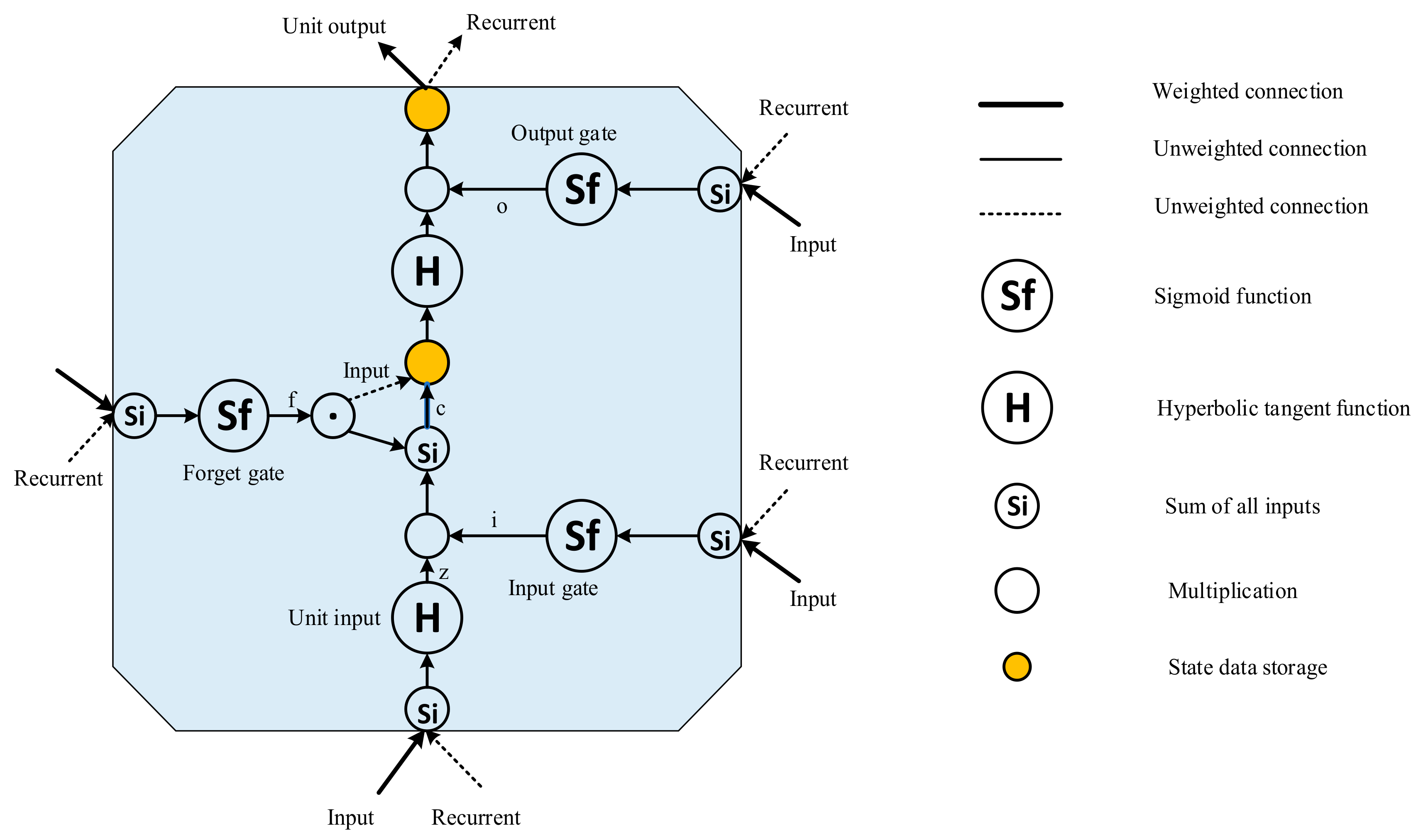
The difference between LSTM and other neural networks is the temporal link between LSTM units in the hidden layer. A typical LSTM cell usually consists of an input gate, an output gate, a forget gate, a unit input, a cell state, and peepholes. The cell state of the LSTM changes over time to preserve long-term memory. LSTM uses storage cells instead of simple neurons to solve the problem of gradient explosion and gradient vanishing.
Figure 8 presents the simplified LSTM units [
27]. It consists of several layers and point-by-point operations that provide information about the state of the LSTM unit and maintain long-term memory through the network and input.
Through the introduction of the memory state and three gates, LSTM is able to find what historical data is worth remembering and what data should be forgotten. In general, LSTM can represent or simulate human behavior, logical development, and the cognitive process of neural tissue more realistically.
To further enhance the accuracy of network prediction, the number of network layer nodes, activation functions, and batch size are optimized by an orthogonal experiment. The primary and secondary relationship can be distinguished from many influential factors to quickly affirm the optimal network parameters. Then, the required number of the experiment is reduced, and the efficiency is intensified. The experimental schemes of the orthogonal experiment are listed in
Table 5.
The activation function is the mechanism by which neurons process and transmit information through the neural network. The activation function helps determine whether we need to activate neurons and the intensity of those neurons signals. Different activation functions may lead to differences in network classification or prediction performance, so we compare three common activation functions including Sigmoid, Relu, and Tanh for training neural networks. For the number of layers in the network, the larger it is, the stronger the learning and expression abilities of the network to data. However, a larger layer node number does not definitely mean a better performance, because on the one hand, it will result in a training cost, and on the other hand, it will result in unnecessary fitting brought by a more complex network structure. So, when setting up the network model, we need to choose an appropriate size of the dataset and network layer node number. Batch Size refers to the number of samples selected once training. Its size affects the optimization degree and speed of the model. A large Batch Size means accurate gradients. However, it may cause enormously different gradients after a certain level, therefore making it difficult to use a global learning rate. An appropriate Batch Size can reduce the number of iterations for network training, improve the training speed, and make the gradient descent direction more accurate. In order to improve the accuracy of the internal leakage prediction, nine calibration schemes of network parameters were constructed through orthogonal tests. The ultimate purpose is to make the predicted result slightly greater than the actual leakage quantity for an effective subsequent risk assessment as well as prediction accuracy.
In
Table 5, the normal multinomial regressive experimental design of three factors and three levels are adopted. The optimization parameters are shown as follows:
The number of network layer nodes are 10, 30, and 50.
Activation functions are sigmoid, relu, and tanh.
Batch sizes are respectively 50, 100, and 200.
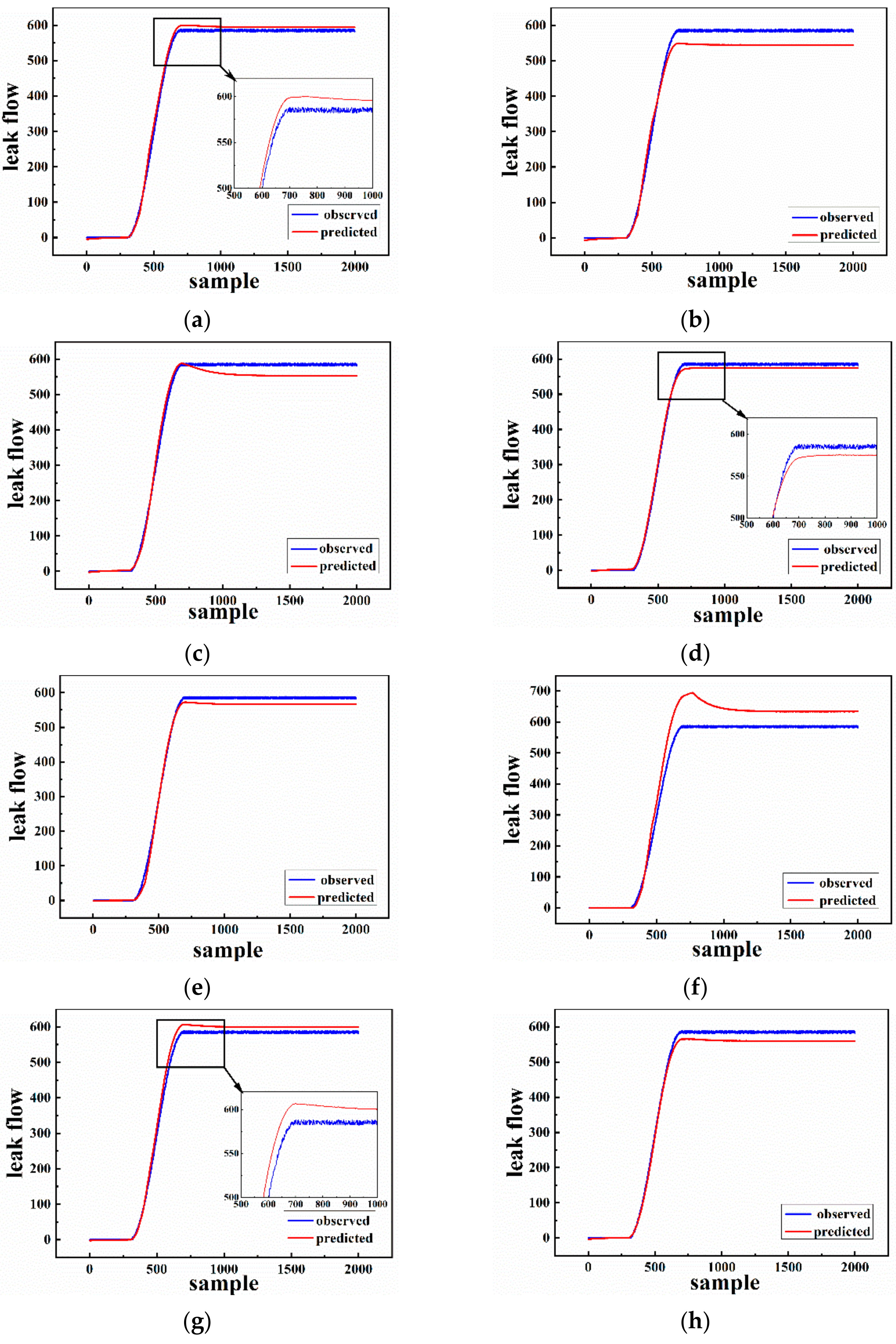
The optimized prediction effect is intuitively shown in
Figure 9. It can be seen that the predictive effect of
Figure 9a,d,g is better than others. However, the predicted value in
Figure 9d is smaller than the observed value overall. So, it may underestimate the harm of risk consequences, resulting in inadequate protection measures preparation and further unnecessary losses. Conversely, the prediction accuracy of
Figure 9a is more excellent than that of
Figure 9g, so the orthogonal experiment of scheme (a) is the most effective. Therefore, five layer nodes, sigmoid activation function, and a Batch Size of 50 are selected as optimal LSTM network parameters in this paper.
4.2. Monitoring Process
On the basis of the analysis in
Section 4.1, adam is select as the optimizer. The network adopts the sigmoid activation function, and its recurrent core adopts the hard-sigmoid function for prediction with the mean absolute error as the loss function. The dropout layer is added to prevent the training process from over fitting.
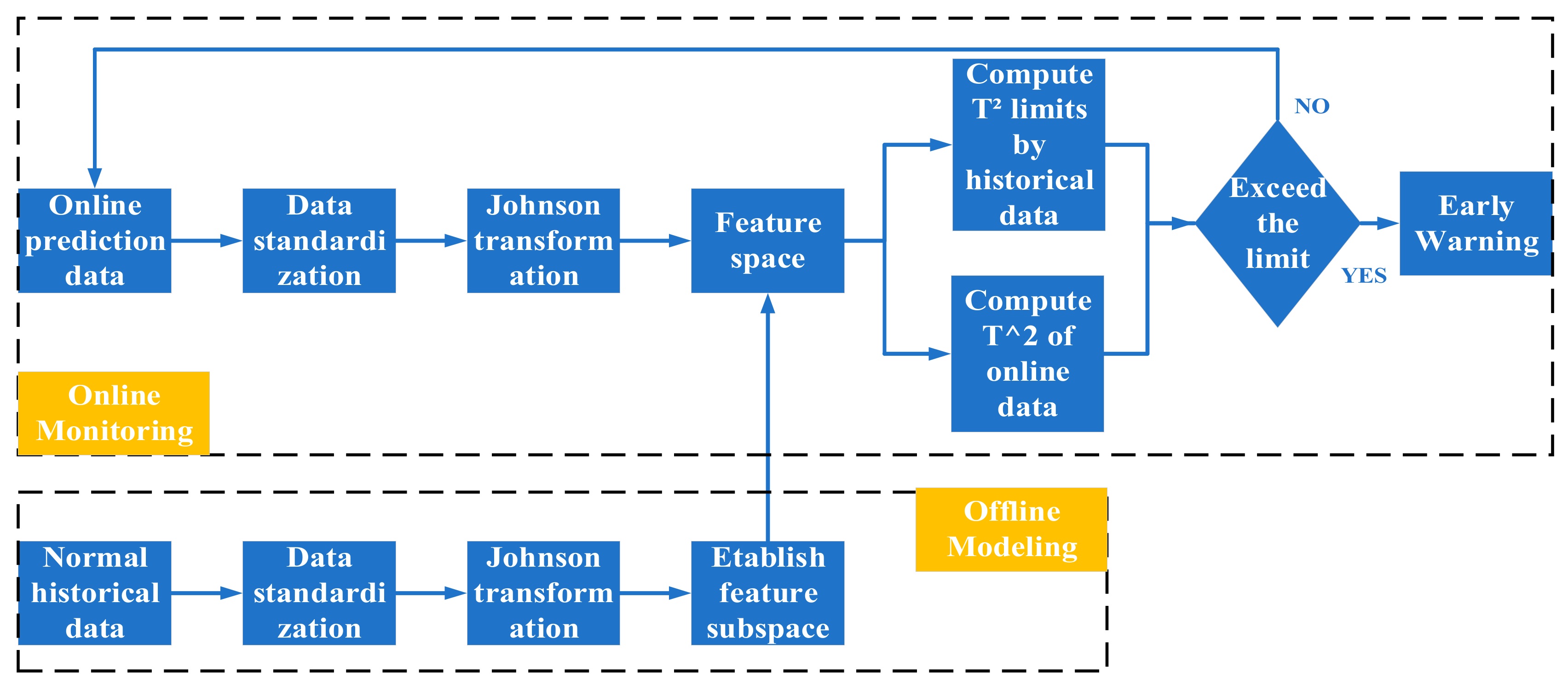
An early warning analysis model is the core of early warning implementation. To improve the timeliness and accuracy, the early warning indicator is selected among data-driven statistic methods. Principal Component Analysis (PCA) is a data-driven process monitoring method that is widely applied in engineering practice. The assumption that the data obeys Gaussian distribution causes its monitoring effect to be poor and the extraction of nonlinear features to be unrobust. In a consequence, Johnson Gaussian transformation is performed on process data to make it obey Gaussian distribution. The implementation steps are similar to PCA. The advantage of this combination is that it well captures the non-Gaussian changes of the process more robustly. The process is shown in
Figure 10.
The monitoring steps are divided into two stages. Stage 1 is offline modeling with following steps: (1) standardize the normal historical process data to make the data have zero mean and unit variance; (2) perform Johnson transformation on the standardized data to make them obey normal distribution; (3) extract the feature vectors and construct the feature space; (4) project the normal data into the feature space and calculate the thresholds of T2. Stage 2 is online monitoring with following steps: (1) standardize the online process data to make it have zero mean and unit variance; (2) perform Johnson transformation on the standardized data to make the data obey normal distribution; (3) project the data into the feature space and calculate the T2 statistics; (4) judge whether the online data of T2 exceed its threshold value. If the threshold is exceeded, go to step 5; otherwise, go to step 6; (5) internal leakage early warning; (6) go back to step 1 and continue to monitor the next set of data.
As an early warning indicator, the
T2 statistic represents the distance between the observed value in the characteristic subspace and the data center. Its calculation formula is given as Equation (1):
where Λ
a represents the diagonal matrix of the diagonal elements corresponding to the previous
a eigenvectors. The threshold formula of
T2 is as shown in Equation (2):
where
Fα(
l, n-l) represents the F distribution with the confidence level of
α, the degree of freedom of
l, and
n − 1,
n is the number of samples in the training set, and
l is the number of selected eigenvectors.
The predicted results of Cases (1)–(4) listed in
Table 4 are shown in
Figure 11. Shown as the dotted red line in
Figure 11, the indicator threshold value four cases are 3.54, 3.36, and 2.56 kg/h, respectively. Prediction curves of Cases (1), (3), and (4) are tightly coincident with observation line. It can be seen that the indicator can early warn of internal leakage when the leakage flow is relatively small. It should be noted that the amount of test data in Case (2) is only 1500. On account of the bad effect compared with the other three cases, we retrain the network with the first 500 data of the test set as the training set.
6. Conclusions
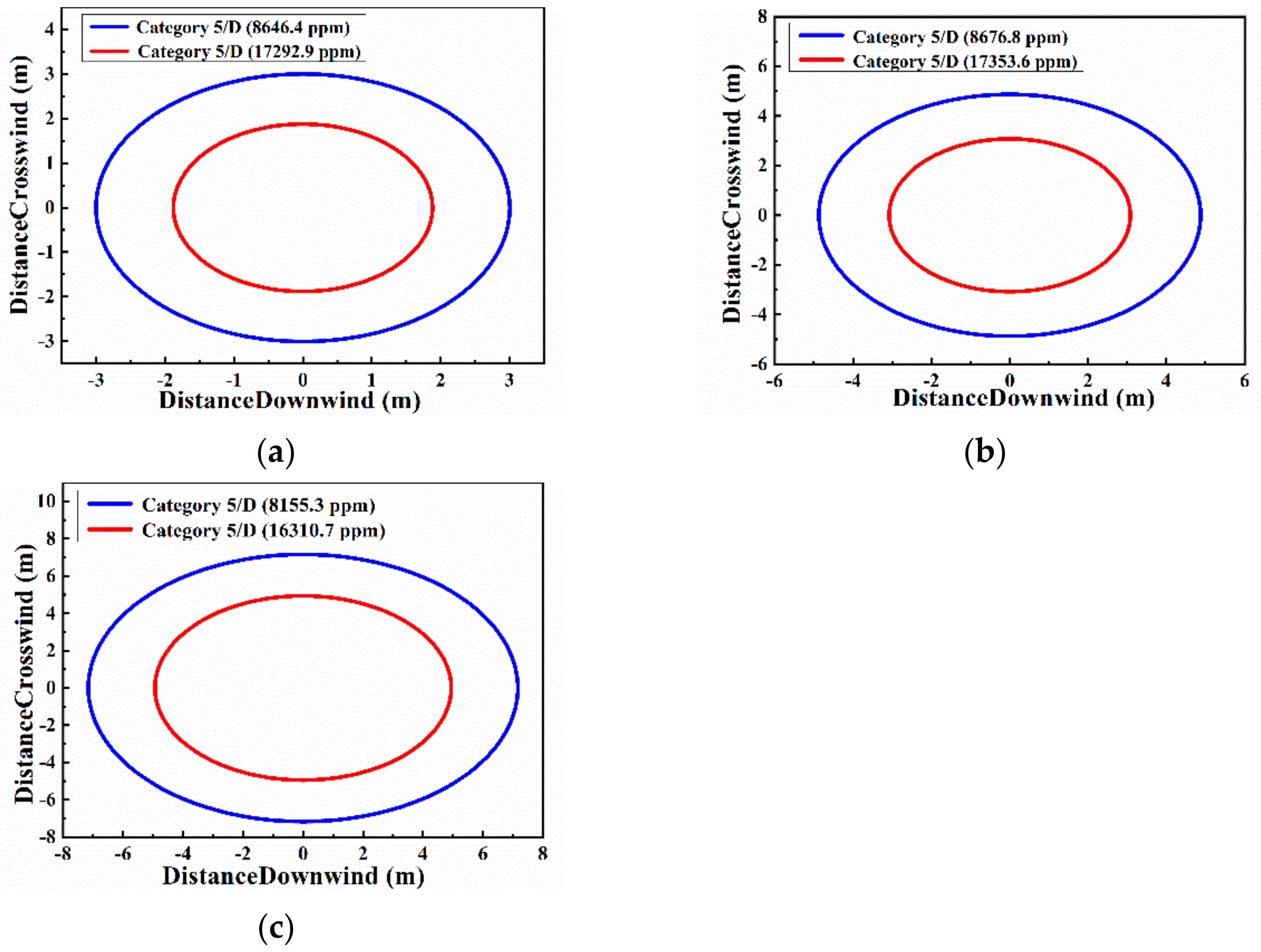
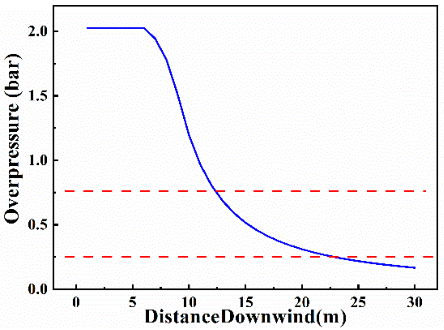
To realize timely and quantitative early warning and risk analysis of internal leakage, a novel intelligent early warning and risk assessment strategy is proposed based on the internal leakage mechanism model. The simulated values of temperature, pressure, and mass flow for each stream are calculated by steady-state simulation with results very close to their real industrial values. The early warning analysis model is established by LSTM, in which PCA is selected for the early warning indicator. The QRA approach is applied to conduct risk assessment, whose results show that the hazard radius of jet fire is proportional to the leakage amount, which is 3.5, 5.5, and 9 m. The radius of the gas concentration exceeding the upper limit of the flash fire is proportional to the amount of leakage, which is 2, 3, and 5 m. The overpressure will cause severe damage to people and property within 23 m. The vapor cloud of organic matters caused by internal leakage will explode if it encounters open fires between 15 and 30m. According to the analysis of dynamic results, the important equipment within 30 m from the explosion center should be coated with fire-retardant coating. Simultaneously, the electrostatic discharge devices should be installed within 30 m of the factory equipment group. At the appropriate location in the factory, the detectors and alarm devices need to be increased.
The dynamically updating risk realized in this paper indicates more effective and real-time warning information. However, due to the limitation of the process, the applicability and reliability of the method need to be verified in a larger process in the future.


 ,
, 


