Author Contributions
Conceptualization, T.E. and M.K.; methodology, T.E. and N.J.; validation, T.E. and N.J.; formal analysis, T.E.; investigation, T.E. and N.J.; writing—original draft preparation, T.E. and N.J.; visualization, T.E. and N.J.; supervision, M.K. All authors have read and agreed to the published version of the manuscript.
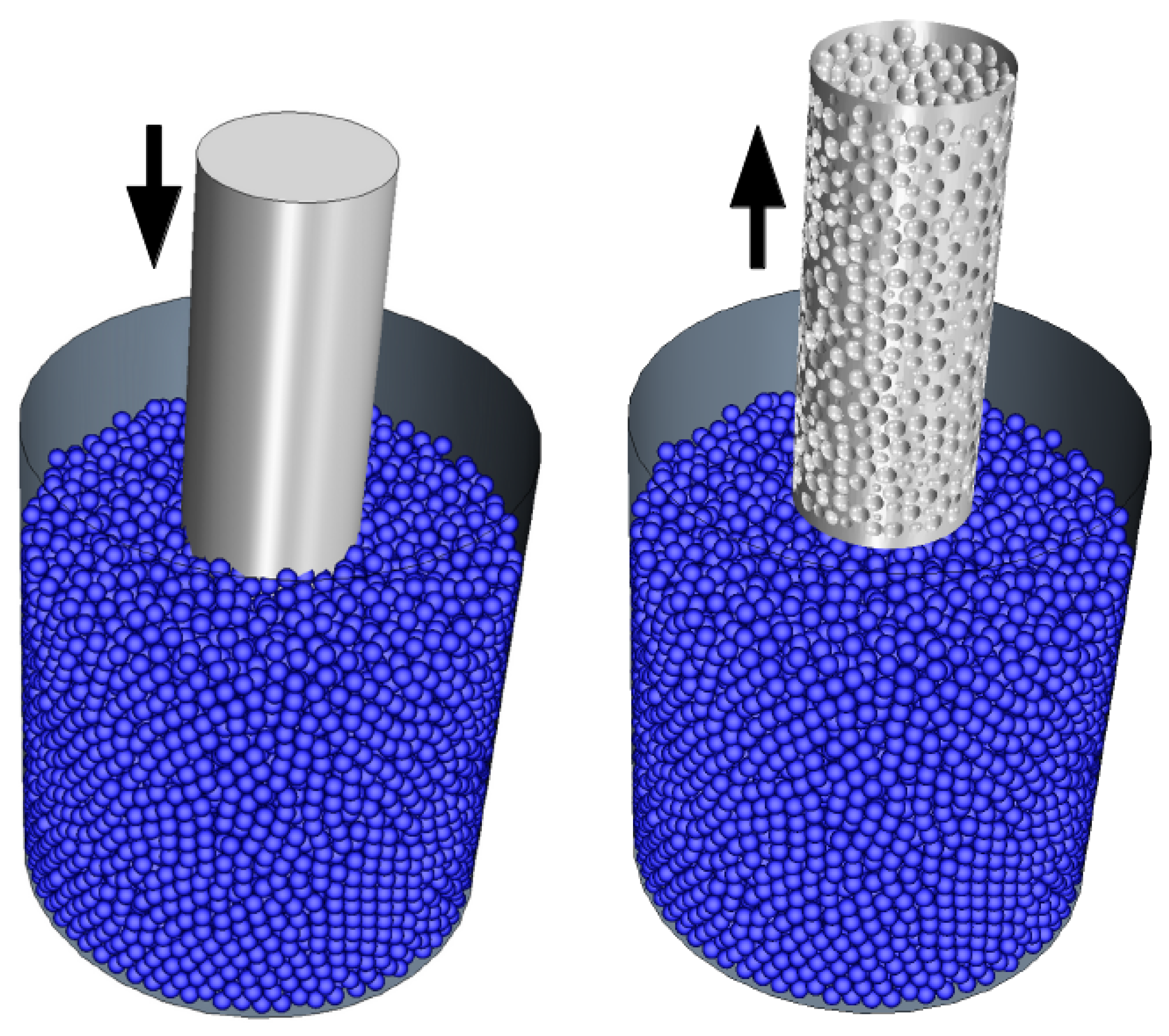
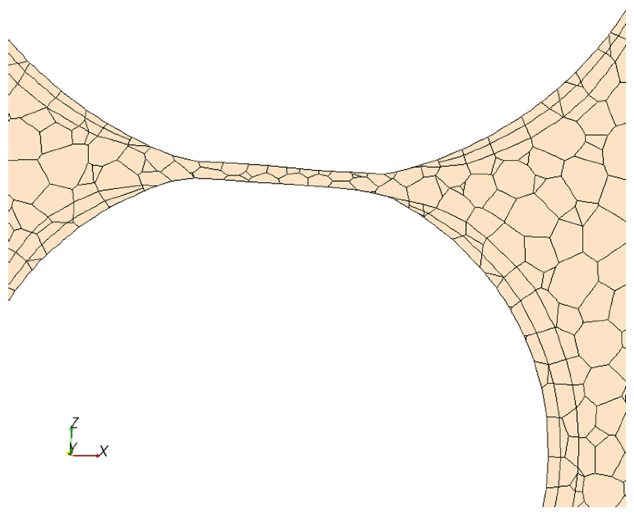
Figure 1.
Local flattening at the contact point of two spherical particles.
Figure 1.
Local flattening at the contact point of two spherical particles.
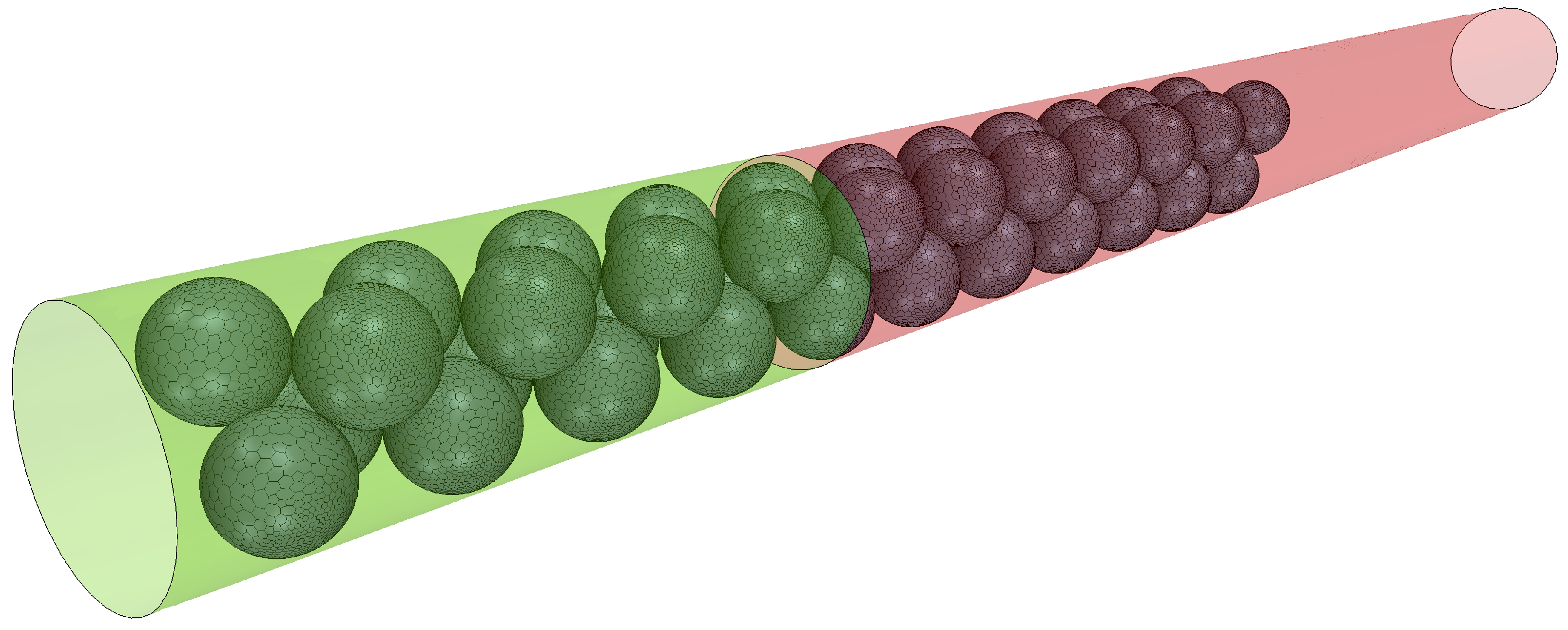
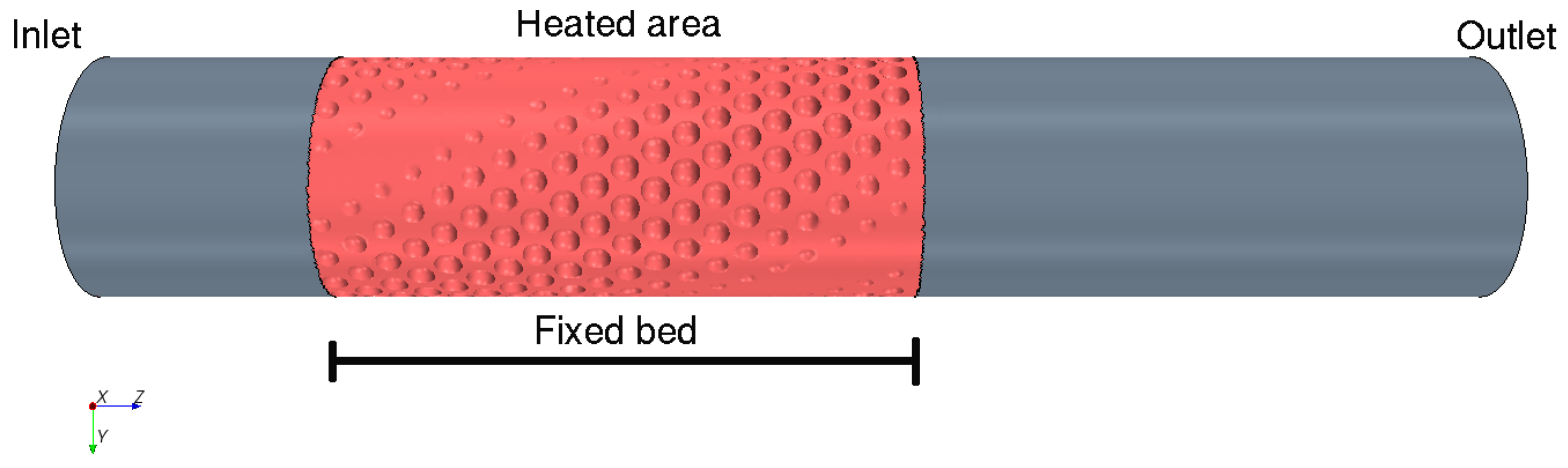
Figure 2.
Reactor geometry overview for a particle diameter ratio of = 8.8: flow direction is from left to right. The red zone marks the heating area (constant temperature K) as well as the fixed bed. The upstream and downstream extrusion to minimize the influence of the inlet and outlet boundary condition is shown in grey.
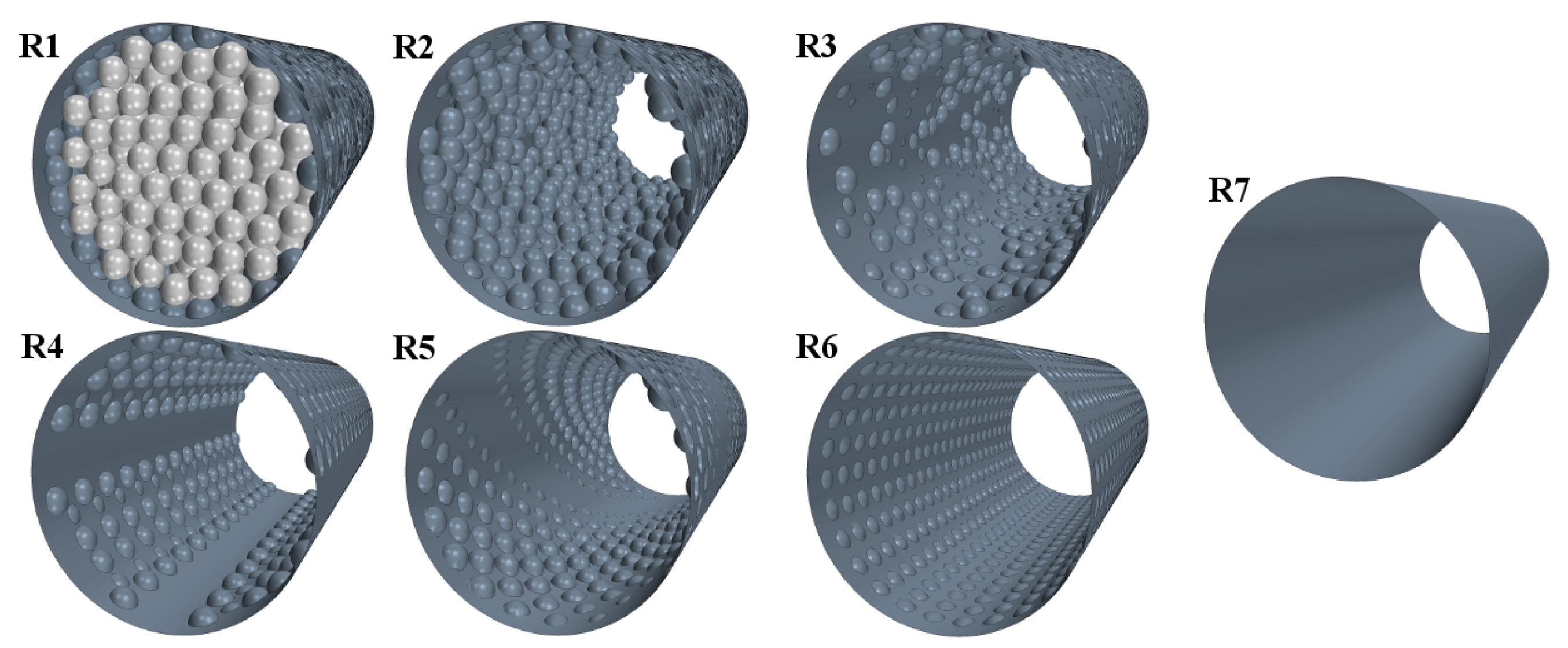
Figure 3.
Investigated wall structure overview: R1—ideal; R2 is like R1, but refilled (later referred to as ideal wall reactor (IWR)); R3 is like R2, but spheres belonging to the wall structure are removed if their centroid resides within the tube; R4–R6—different regular arrangements (R5 is later referred to as oscillating wallstructure reactor (OWR)); R7—plain wall (later referred to as plain wall reactor (PWR)).
Figure 4.
Outline of the process for generating an irregular wall structure.
Figure 4.
Outline of the process for generating an irregular wall structure.
Figure 5.
Sketch of the experimental and numerical setup of the pre-study. The heating zone starts behind the light green zone, flow direction is from left to right.
Figure 5.
Sketch of the experimental and numerical setup of the pre-study. The heating zone starts behind the light green zone, flow direction is from left to right.
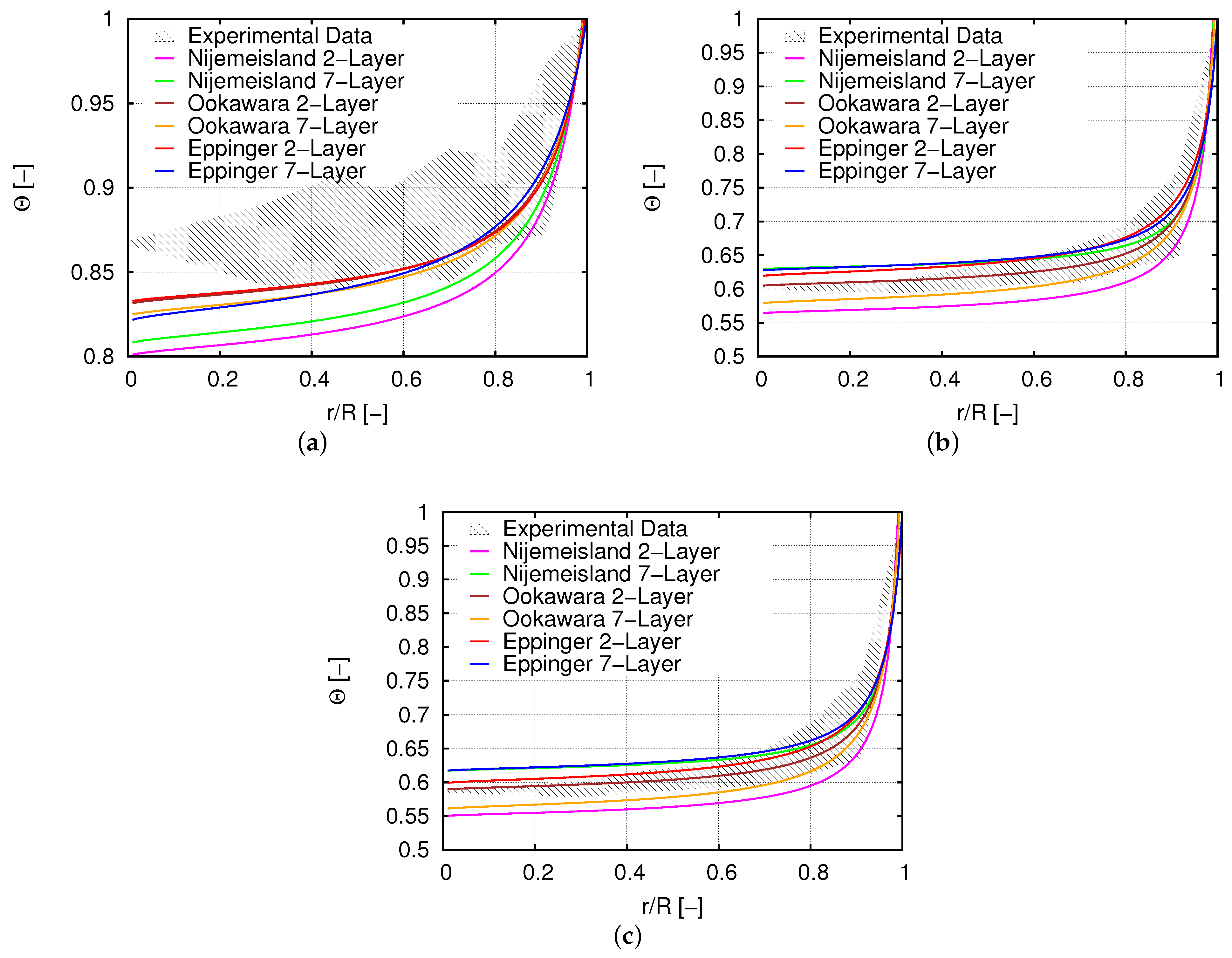
Figure 6.
(a–c) Comparison of temperature data at the outlet of the packed bed for different contact point methods and experimental data for Re = 986; (d) best-fit curves based on the results from (a–c).
Figure 6.
(a–c) Comparison of temperature data at the outlet of the packed bed for different contact point methods and experimental data for Re = 986; (d) best-fit curves based on the results from (a–c).
Figure 7.
Best-fit curves based on the simulation results. (a) Best-fit curves based on the simulation results for Re = 373, (b) Best-fit curves based on the simulation results for Re = 1724, (c) Best-fit curves based on the simulation results for Re = 1922.
Figure 7.
Best-fit curves based on the simulation results. (a) Best-fit curves based on the simulation results for Re = 373, (b) Best-fit curves based on the simulation results for Re = 1724, (c) Best-fit curves based on the simulation results for Re = 1922.
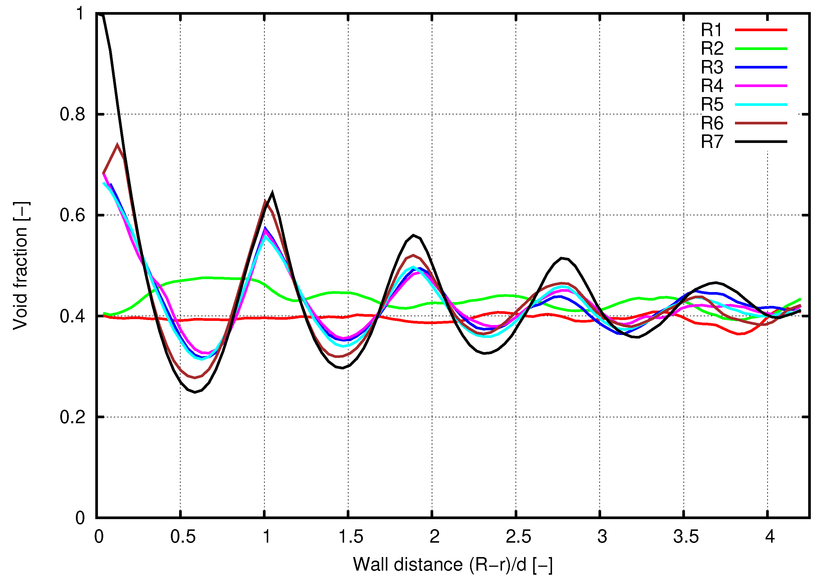
Figure 8.
Averaged radial void fraction profiles for different wall structures.
Figure 8.
Averaged radial void fraction profiles for different wall structures.
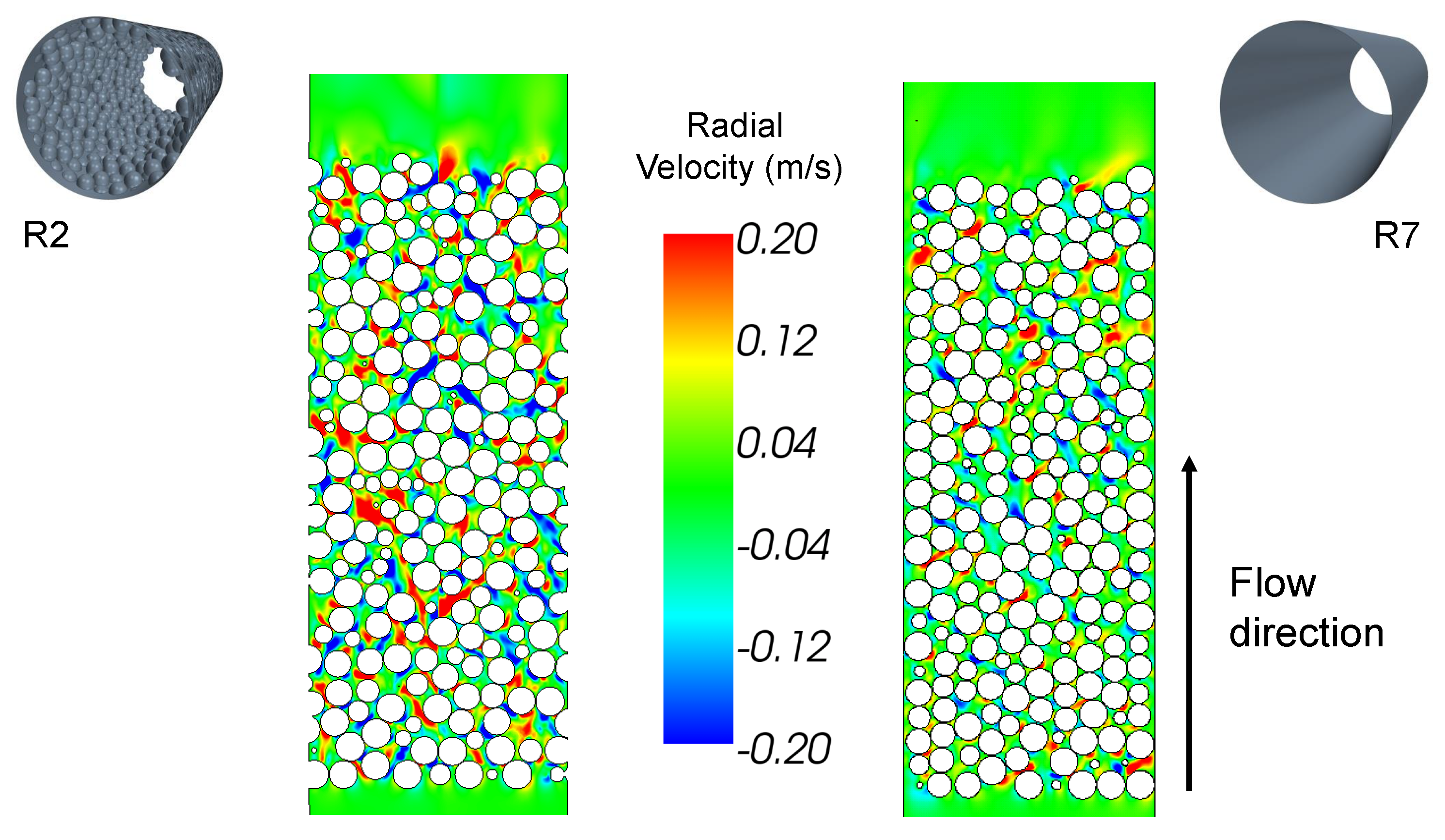
Figure 9.
Comparison of the local radial velocity between configuration R2 with wall structure and R7 for a -ratio of 8.8.
Figure 9.
Comparison of the local radial velocity between configuration R2 with wall structure and R7 for a -ratio of 8.8.
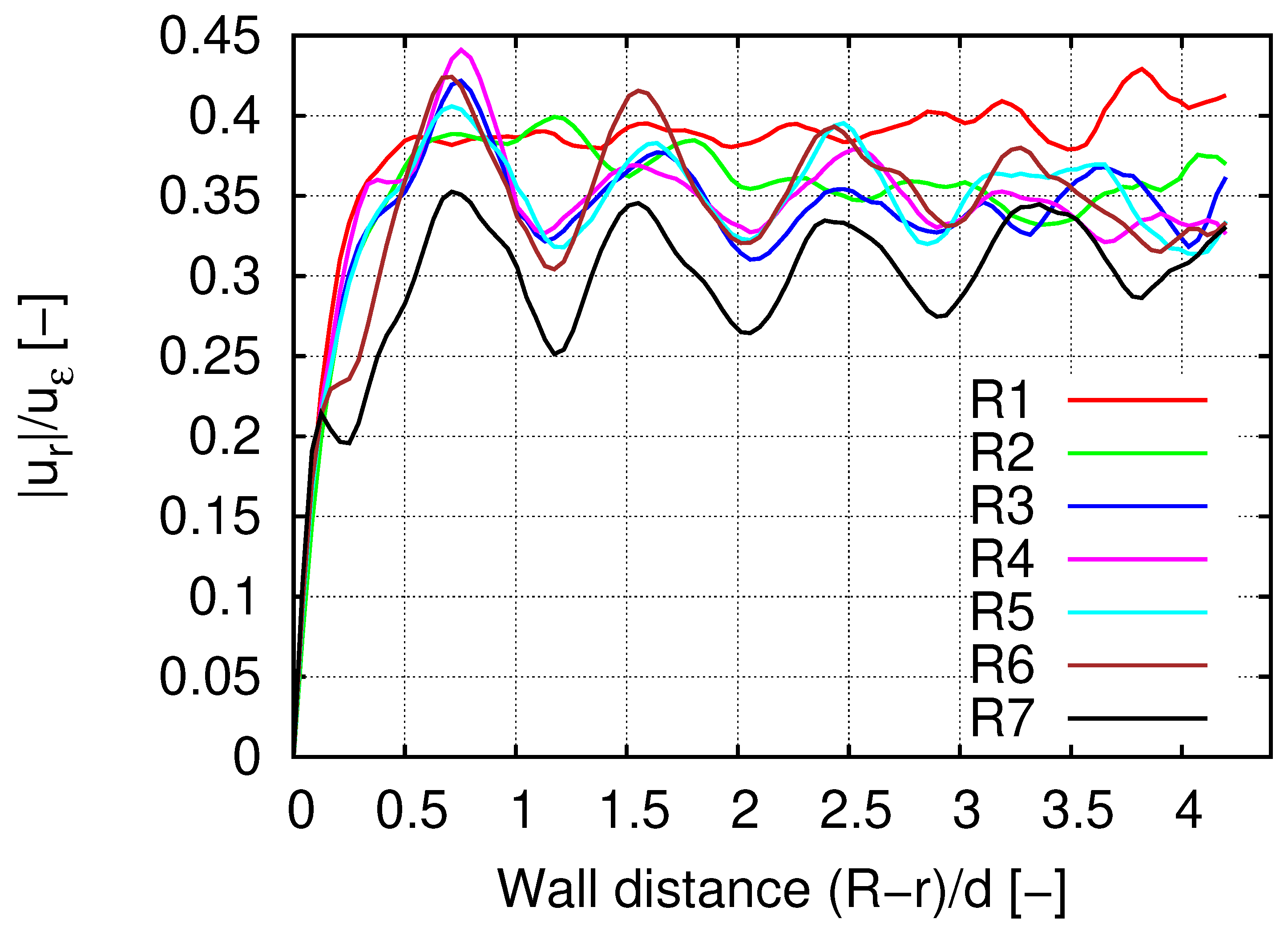
Figure 10.
Averaged (circumferential and over the bed height) magnitude of the radial velocity component . A significant increase for configurations with wall structure can be observed compared to R7 (plain wall).
Figure 10.
Averaged (circumferential and over the bed height) magnitude of the radial velocity component . A significant increase for configurations with wall structure can be observed compared to R7 (plain wall).
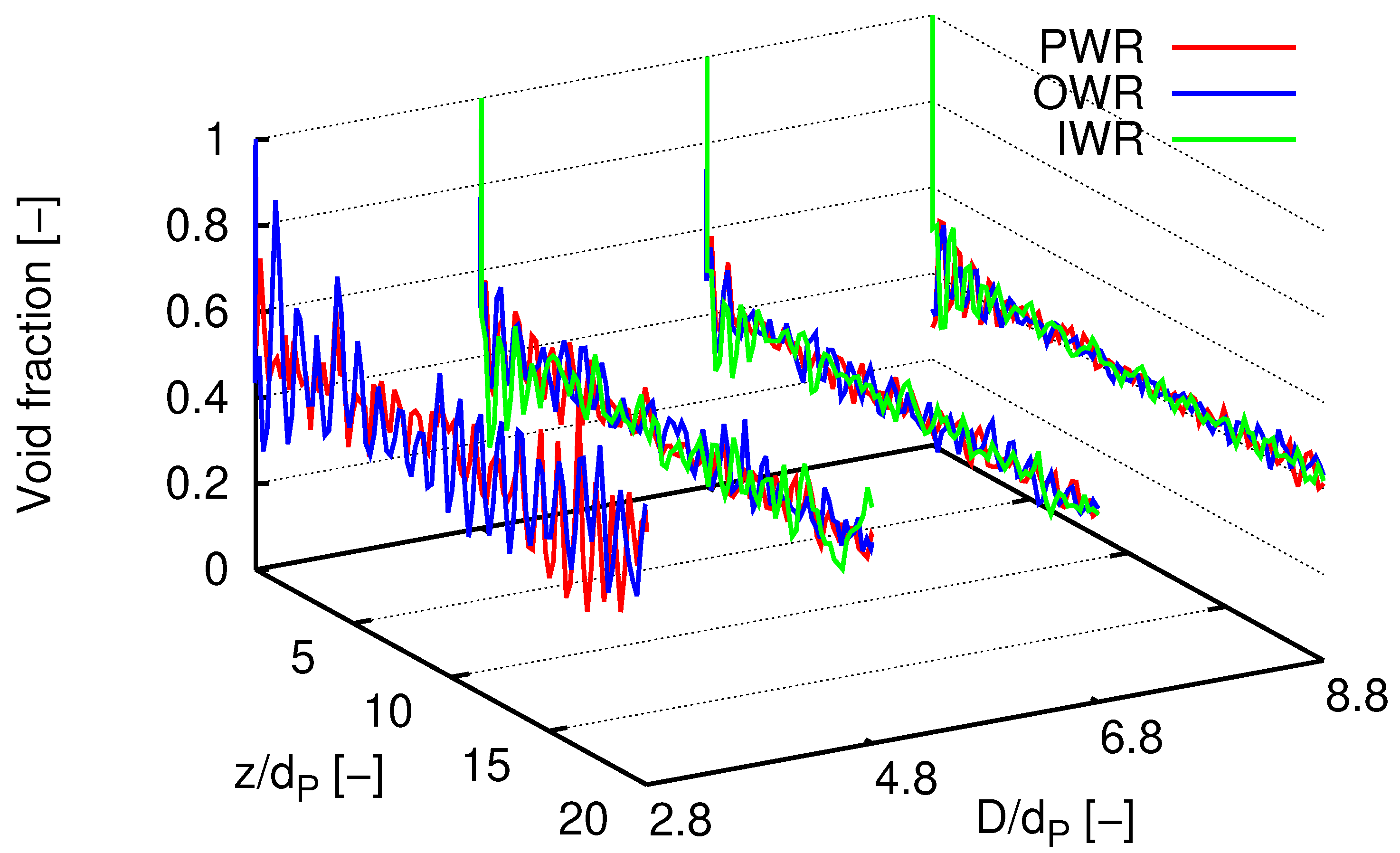
Figure 11.
Axial void fraction distributions.
Figure 11.
Axial void fraction distributions.
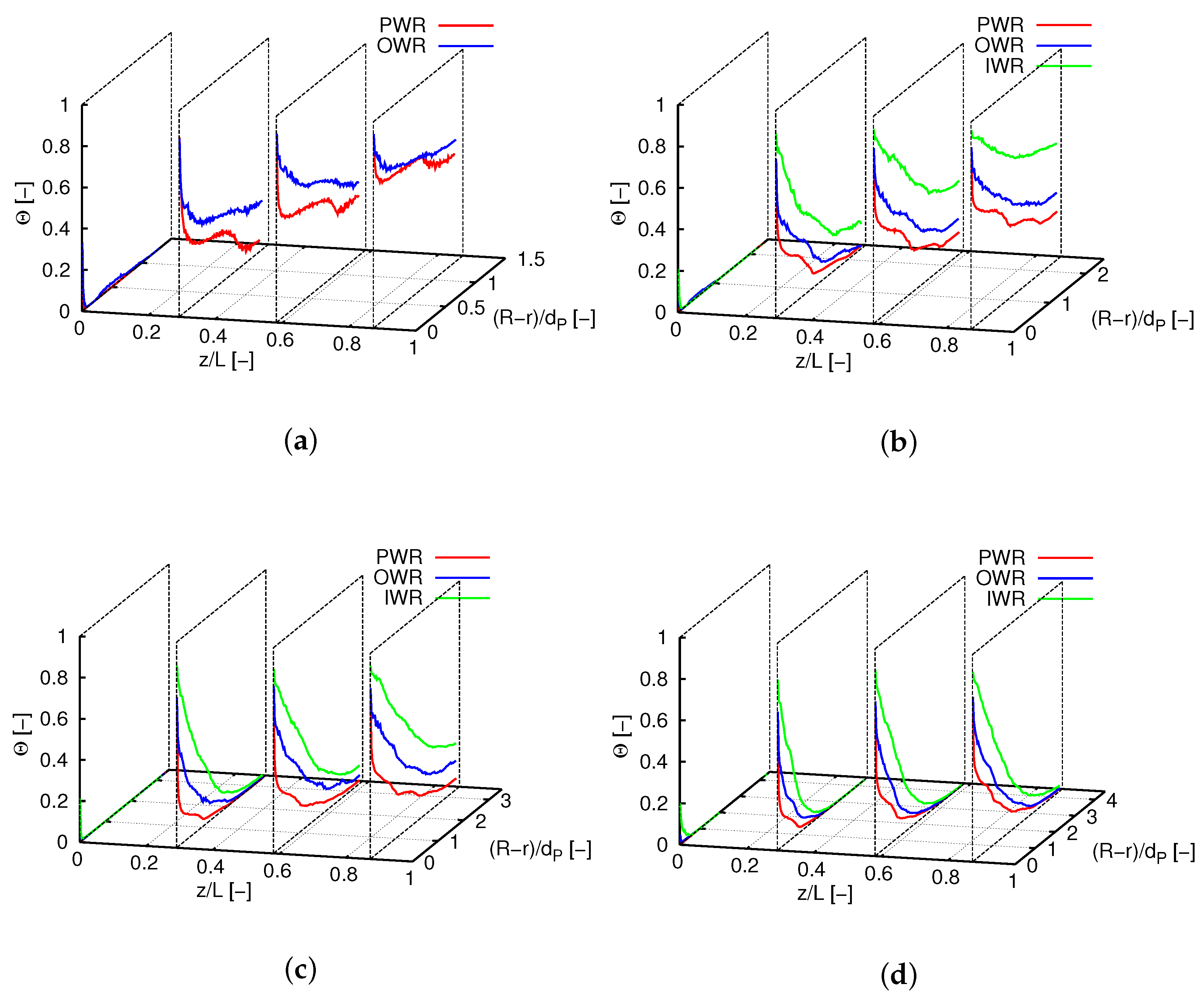
Figure 12.
Radial void fraction distributions.
Figure 12.
Radial void fraction distributions.
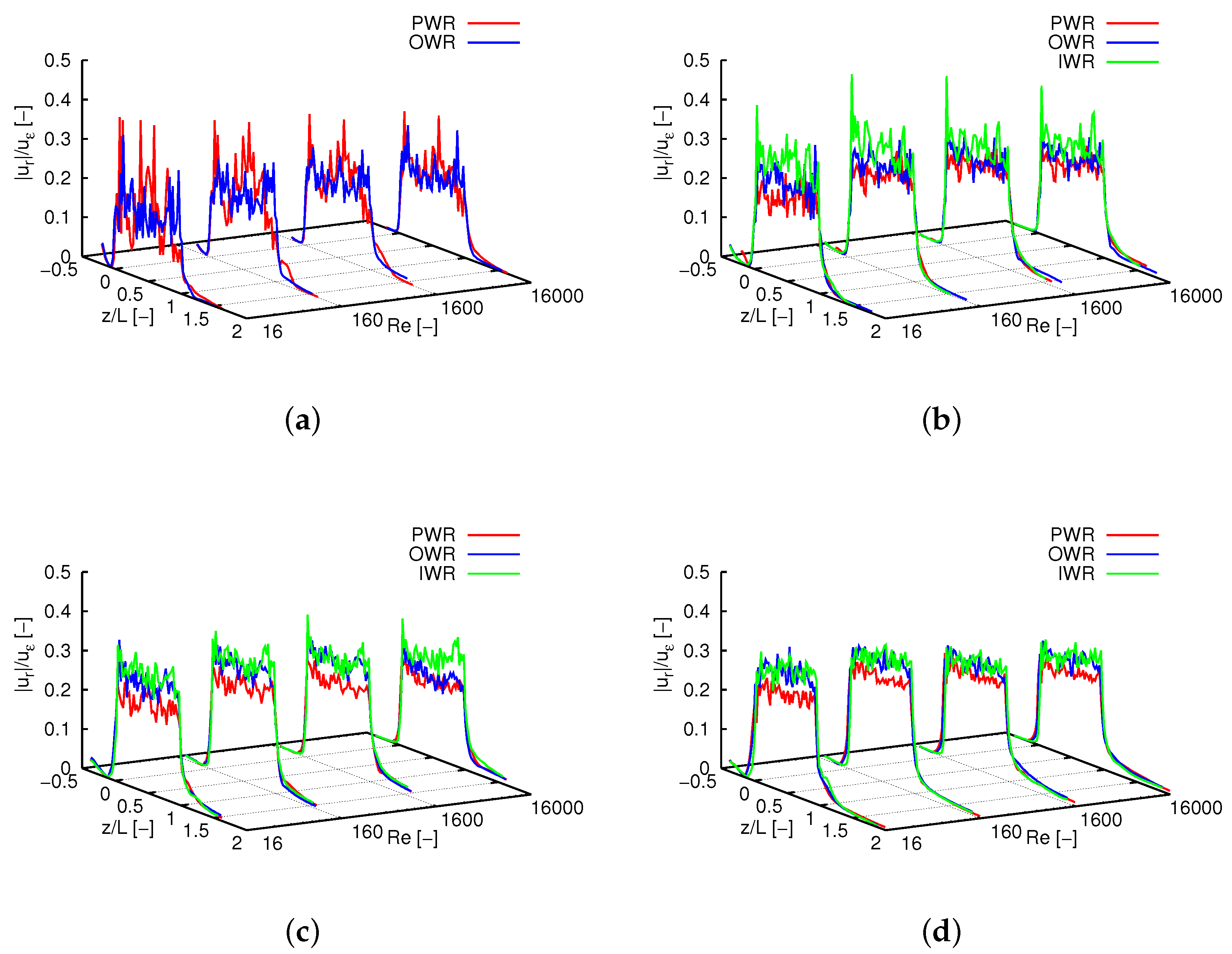
Figure 13.
Axial progression of the area averaged magnitude of the radial velocity normalized with the interstitial velocity. (a) , (b) , (c) , (d) .
Figure 13.
Axial progression of the area averaged magnitude of the radial velocity normalized with the interstitial velocity. (a) , (b) , (c) , (d) .
Figure 14.
Comparison of the temperature distribution in a cross section through the center axis of the reactor.
Figure 14.
Comparison of the temperature distribution in a cross section through the center axis of the reactor.
Figure 15.
Radial temperature profiles for Re = 1600. (a) , (b) , (c) , (d) .
Figure 15.
Radial temperature profiles for Re = 1600. (a) , (b) , (c) , (d) .
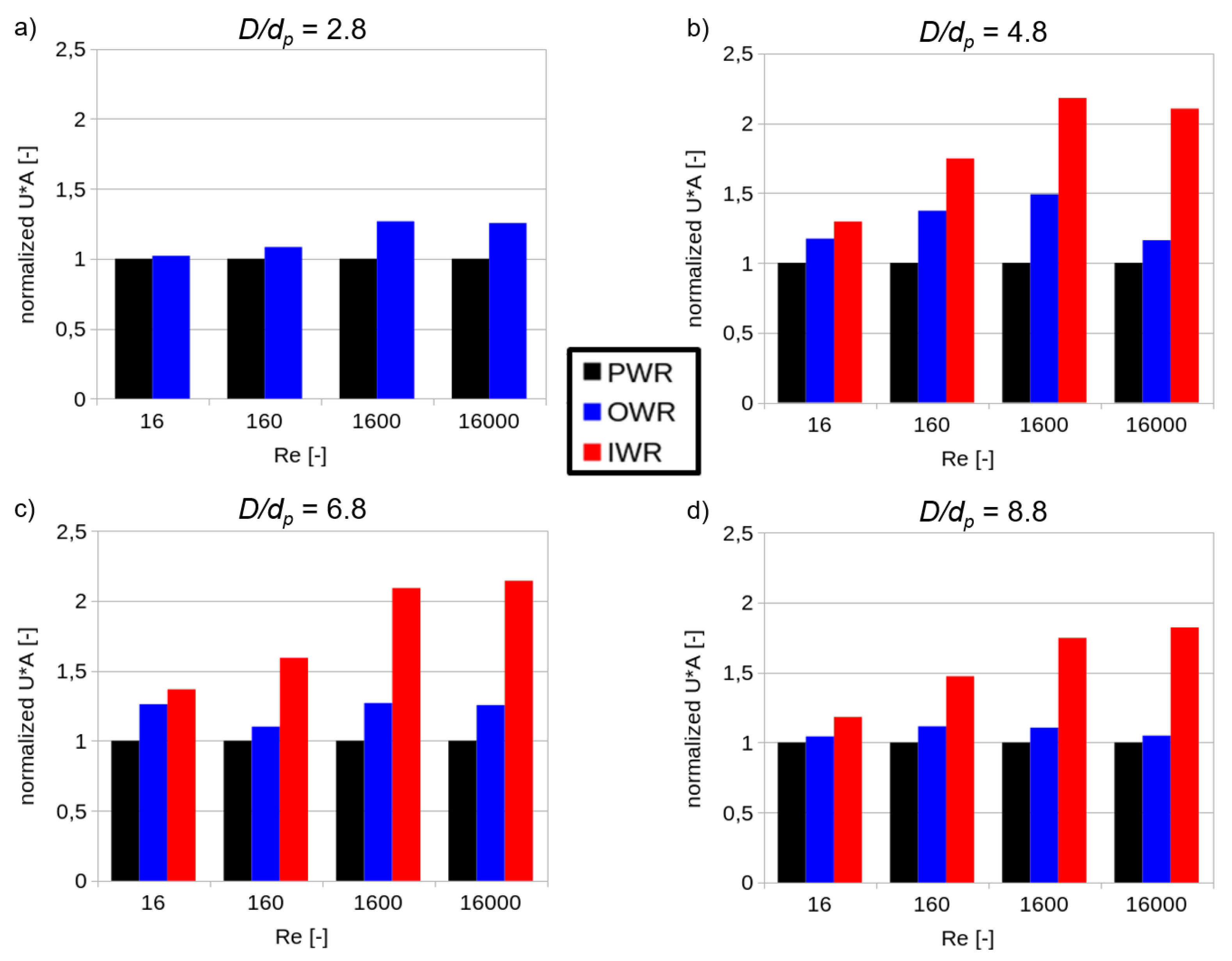
Figure 16.
Comparison of normalized U*A as a measure for the thermal performance for varying -ratios, Reynolds numbers and wall structures.
Figure 16.
Comparison of normalized U*A as a measure for the thermal performance for varying -ratios, Reynolds numbers and wall structures.
Table 1.
Used parameters for the discrete element method (DEM) simulation.
Table 1.
Used parameters for the discrete element method (DEM) simulation.
| Property | Unit | Value |
|---|
| Diameter | m | 0.025 |
| Density | kg/ | 2500 |
| Coefficient of restitution, normal | − | 0.9 |
| Coefficient of restitution, tangential | − | 0.5 |
| Poisson coefficient | − | 0.0235 |
| Young’s modulus | Pa | 78.5E9 |
| Sliding friction coefficient | − | 0.2 |
| Rolling friction coefficient | − | 0.002 |
Table 2.
Settings of the meshing parameters.
Table 2.
Settings of the meshing parameters.
| Property | Value |
|---|
| Particle Diameter | 0.025 m |
| Base size (bs) | d |
| Surface edge size (ses) on spheres | 0.04–0.10 |
| Surface grow rate | 1.3 |
| Number of prism layers | 2 |
| Thickness of the prism layers | 0.03 |
| Minimum distance between two surfaces | 0.12 ses |
Table 3.
Parameters and boundary conditions used for the computational fluid dynamics (CFD) simulations.
Table 3.
Parameters and boundary conditions used for the computational fluid dynamics (CFD) simulations.
| Geometrical Properties |
|---|
| Particle diameter | 0.025 m |
| Bed height | 0.55 m |
| Diameter ratio | 2.8, 4.8, 6.8, 8.8 |
| Fluid Properties (Air) |
| Dynamic viscosity | 1.85508E-5 Pa s |
| Molecular weight | 28.9664 g/mol |
| Specific heat | 1003.62 J/kg K |
| Thermal conductivity | 0.0260305 W/m s |
| Solid Properties (Glass) |
| Density | 2500.0 kg/ |
| Specific heat | 750.0 J/kg K |
| Thermal conductivity | 1.4 W/m s |
| Boundary Conditions |
| Pressure outlet | 0.0 Pa |
| Inlet temperature | 298.0 K |
| Heated wall temperature | 373.0 K |
| Inlet velocity | 0.01 m/s, 0.1 m/s, 1.0 m/s, 10.0 m/s |
| Particle Reynolds number | 16, 160, 1600, 16,000 |
Table 4.
Settings for the heat transfer validation simulation in
Section 2.6.
Table 4.
Settings for the heat transfer validation simulation in
Section 2.6.
| Property | Value |
|---|
| 0.026 W/(m·K) |
| 0.242 W/(m·K) |
| 1.225 kg / |
| 1300 kg / |
| 1003.6 J/(kg·K) |
| 1000 J/(kg·K) |
| 298 K |
| 383 K |
Table 5.
Bed void fraction.
Table 5.
Bed void fraction.
| | Diameter Ratio |
|---|
| 2.8 | 4.8 | 6.8 | 8.8 |
|---|
|
Plain Wall Reactor (PWR)
| 0.524 | 0.451 | 0.443 | 0.421 |
|
Oscillating Wall Reactor (OWR)
| 0.528 | 0.464 | 0.442 | 0.423 |
|
Ideal Wall Reactor (IWR)
| – | 0.445 | 0.435 | 0.421 |
Table 6.
Axially averaged mean radial velocity magnitude.
Table 6.
Axially averaged mean radial velocity magnitude.
| | Diameter Ratio |
|---|
| |
2.8
|
4.8
|
6.8
|
8.8
|
|---|
|
Re
|
PWR
|
OWR
|
IWR
|
PWR
|
OWR
|
IWR
|
PWR
|
OWR
|
IWR
|
PWR
|
OWR
|
IWR
|
|---|
| 16 | 0.181 | 0.177 | – | 0.210 | 0.246 | 0.297 | 0.226 | 0.274 | 0.295 | 0.240 | 0.290 | 0.298 |
| 160 | 0.202 | 0.195 | – | 0.237 | 0.261 | 0.306 | 0.242 | 0.283 | 0.302 | 0.256 | 0.296 | 0.303 |
| 1600 | 0.205 | 0.197 | – | 0.230 | 0.248 | 0.281 | 0.219 | 0.272 | 0.278 | 0.233 | 0.257 | 0.262 |
| 16,000 | 0.188 | 0.183 | – | 0.204 | 0.223 | 0.257 | 0.196 | 0.209 | 0.256 | 0.210 | 0.242 | 0.248 |
Table 7.
Calculated thermal entry length.
Table 7.
Calculated thermal entry length.
| | Diameter Ratio |
|---|
| |
2.8
|
4.8
|
6.8
|
8.8
|
|---|
|
Re
|
PWR
|
OWR
|
IWR
|
PWR
|
OWR
|
IWR
|
PWR
|
OWR
|
IWR
|
PWR
|
OWR
|
IWR
|
|---|
| 16 | 0.006 | 0.000 | – | 0.000 | 0.006 | 0.000 | 0.000 | 0.000 | 0.000 | 0.000 | 0.000 | 0.000 |
| 160 | 0.044 | 0.006 | – | 0.033 | 0.033 | 0.011 | 0.105 | 0.078 | 0.066 | 0.170 | 0.159 | 0.165 |
| 1600 | 0.050 | 0.022 | – | 0.116 | 0.116 | 0.072 | 0.281 | 0.221 | 0.122 | 0.461 | 0.428 | 0.352 |
| 16,000 | 0.189 | 0.105 | – | 0.237 | 0.199 | 0.116 | 0.447 | 0.354 | 0.304 | | | |


