
Efficient Two-Step Parametrization of a Control-Oriented Zero-Dimensional Polymer Electrolyte Membrane Fuel Cell Model Based on Measured Stack Data


Abstract
1. Introduction
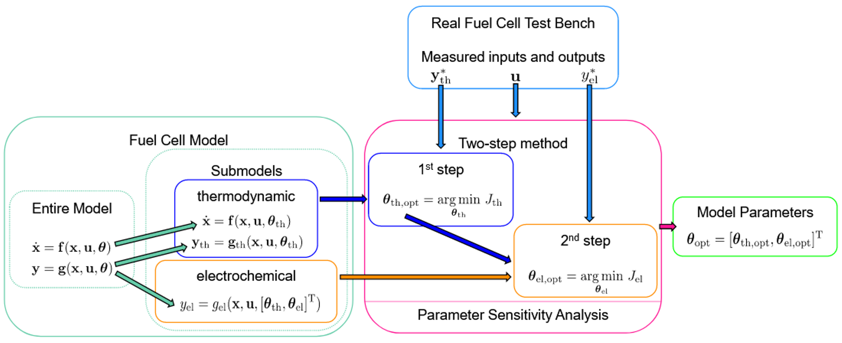
2. Fuel Cell Model
2.1. Model Description
2.2. Model Reduction
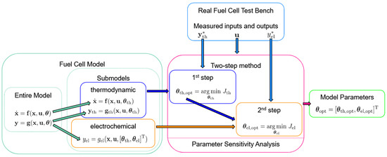
3. Two-Step Parametrization Method
3.1. Key Idea
3.2. Parameter Sensitivity Analysis
3.3. Procedure
- Thermodynamic submodel
- (a)
- Parameter sensitivity analysis with respect to the thermodynamic parameters yields a subset with the most significant parameters , where holds.
- (b)
- Parametrization with respect to the most significant parameters yields the optimized parameters . The least significant parameters are kept constant at their initial values.
- Electrochemical submodel
- (a)
- Solve thermodynamic submodel using the optimized thermodynamic parameters and store the resulting model states for further usage.
- (b)
- Parameter sensitivity analysis with respect to the electrochemical parameters yields a subset with the most significant parameters , where holds.
- (c)
- Parametrization with respect to the most significant parameters yields the optimized parameters . The least significant parameters are kept constant at their initial values.
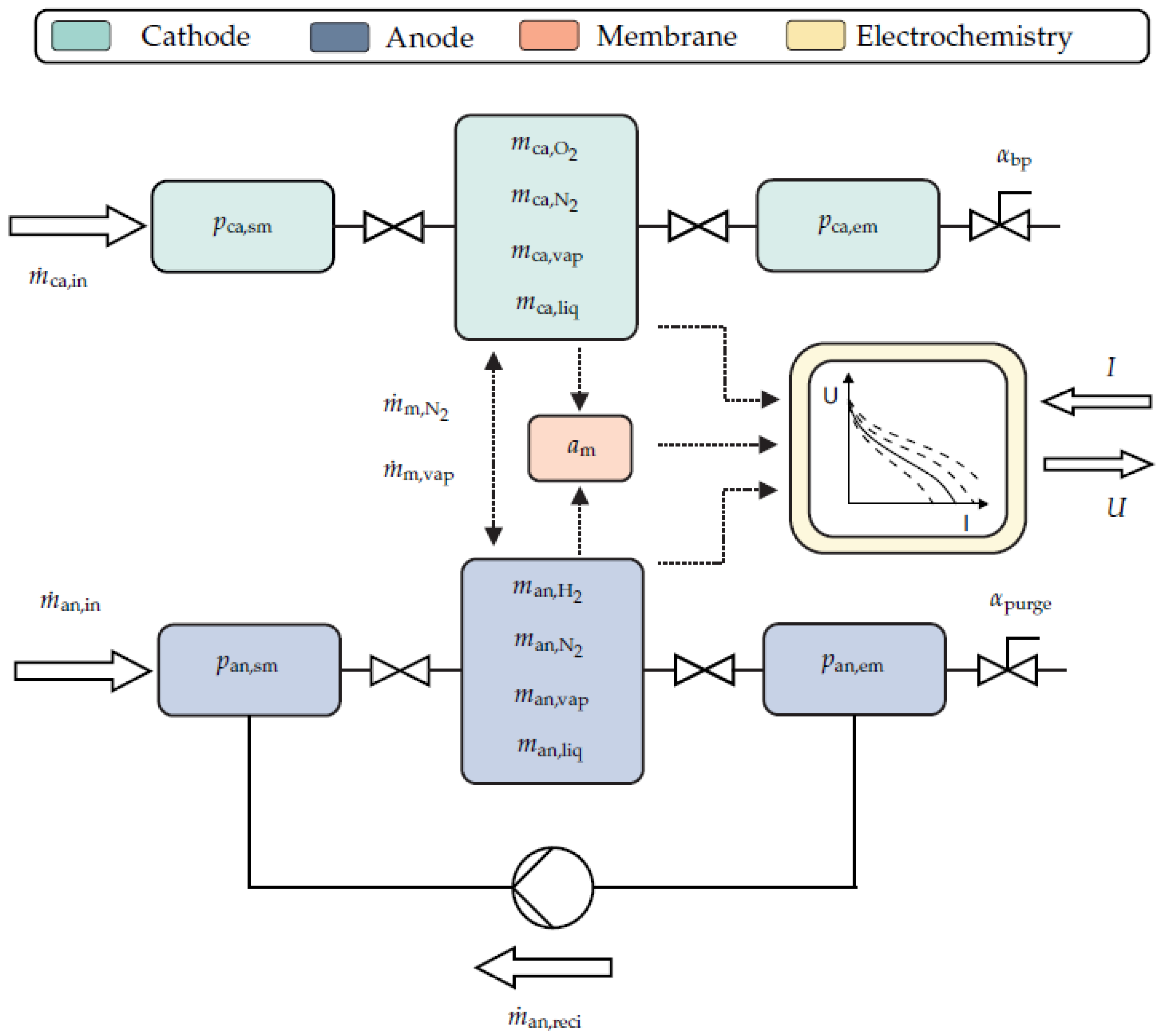
3.4. Validation of Method
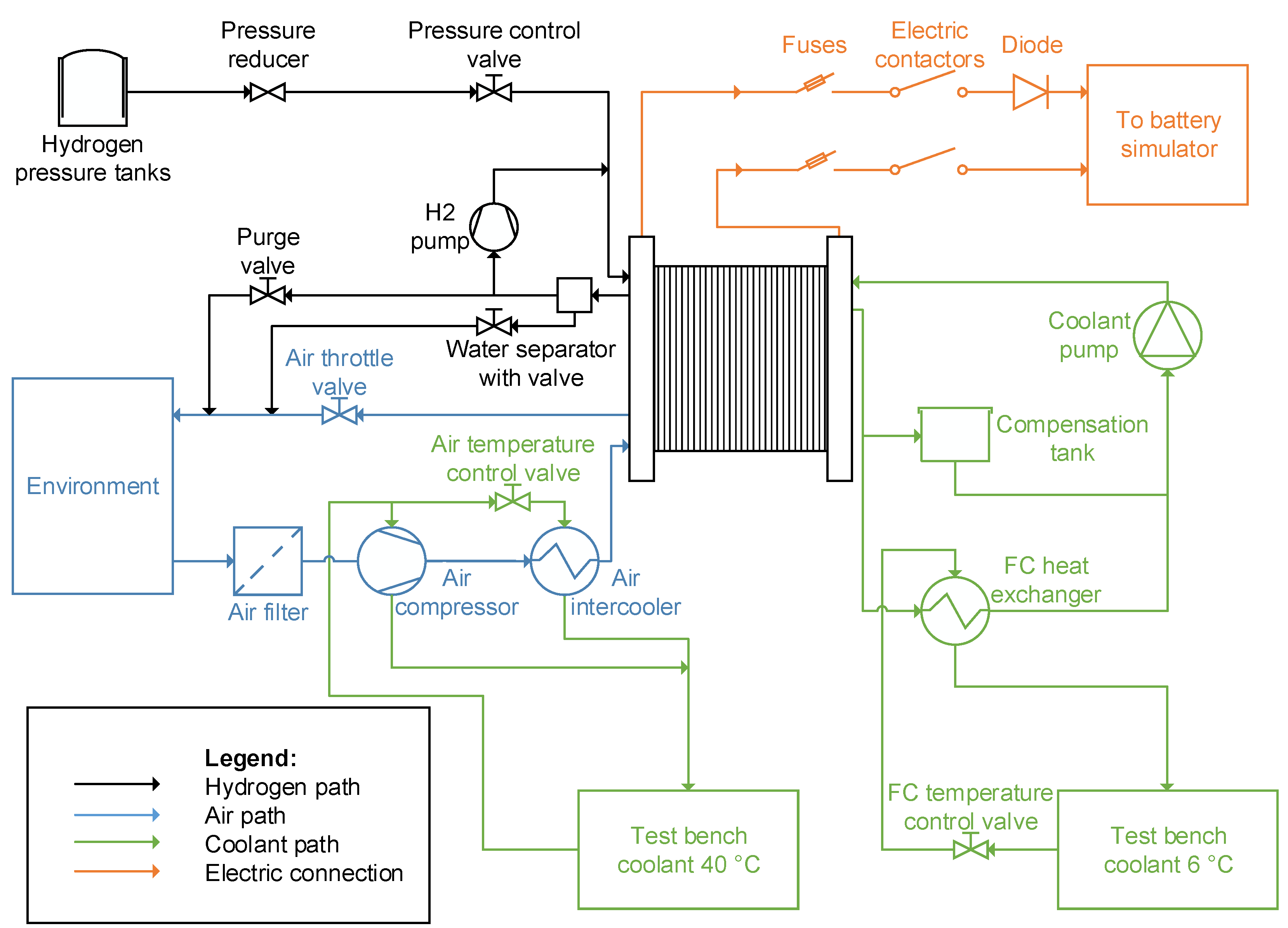
4. Experimental Setup
4.1. Media Supply
4.2. Cooling Circuits
4.3. Test Bench Control System
4.4. Experimental Tests and Operating Conditions
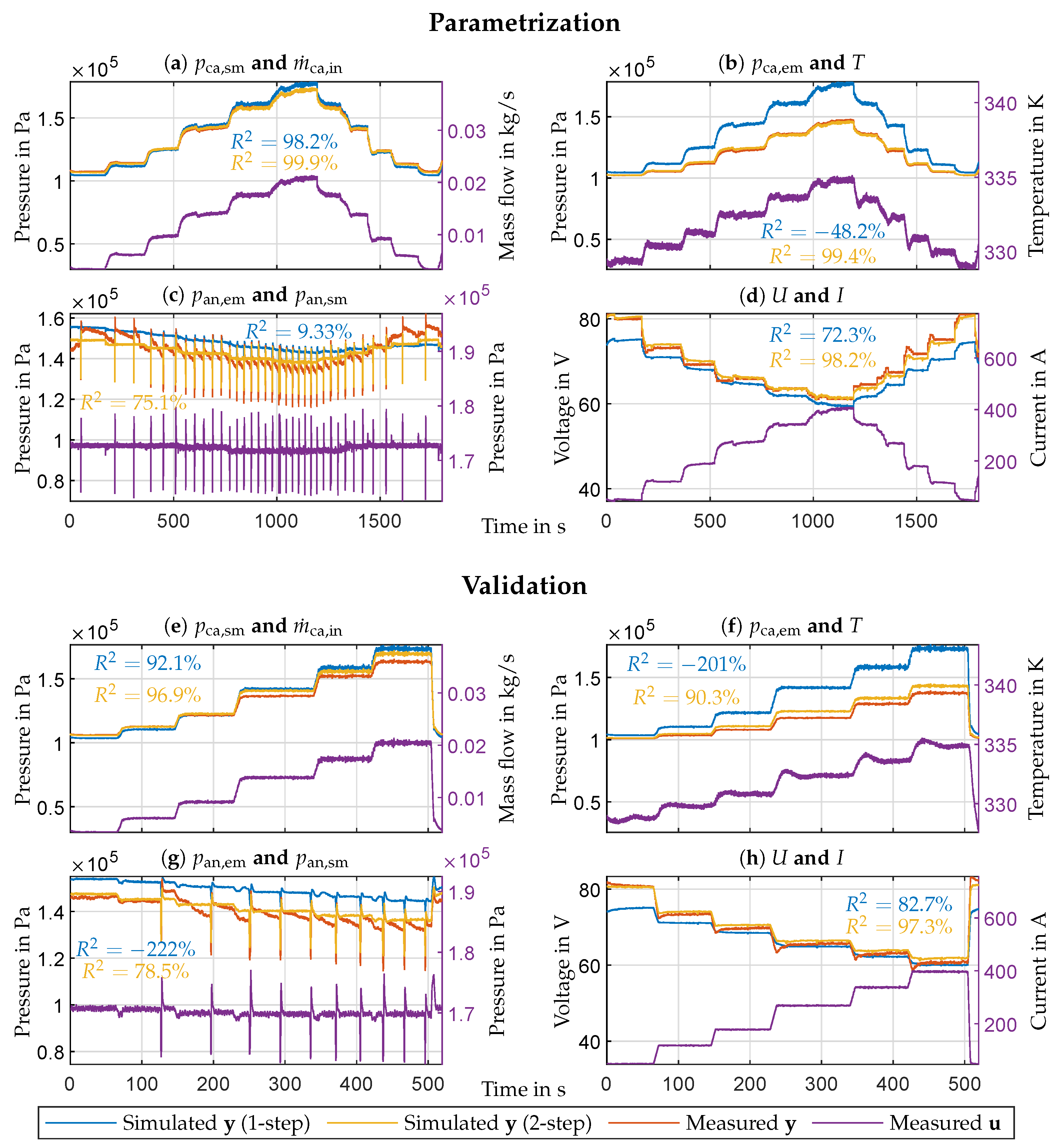
5. Results and Discussion
5.1. Results
5.2. Discussion
6. Conclusions
Author Contributions
Funding
Institutional Review Board Statement
Informed Consent Statement
Data Availability Statement
Acknowledgments
Conflicts of Interest
Abbreviations
| FC | Fuel cell |
| FIM | Fisher information matrix |
| ODE | Ordinary differential equation |
| PEMFC | Polymer electrolyte membrane fuel cell |
| SVD | Singular value decomposition |
Nomenclature
| Subscripts | ||
| 0 | Initial | |
| Activation | ||
| Anode | ||
| Atmosphere | ||
| Backpressure | ||
| Cathode | ||
| Center manifold | ||
| Electrochemical | ||
| Exit manifold | ||
| Hydrogen | ||
| Inflow | ||
| Leakage | ||
| Liquid water | ||
| Least significant | ||
| Maximum | ||
| Minimum | ||
| Most significant | ||
| Membrane | ||
| Nitrogen | ||
| Normalized | ||
| Oxygen | ||
| Optimized | ||
| Outflow | ||
| Permeability | ||
| Purge | ||
| Recirculation | ||
| Supply manifold | ||
| Thermodynamic | ||
| Vapour | ||
| i | Running index for parameters | |
| k | Sampling instant | |
| l | Running index for singular values | |
| Symbols | ||
| Valve position | 1 | |
| Output parameter sensitivity matrix | ||
| Output parameter sensitivity vector | ||
| Singular value matrix | ||
| Prediction error covariance matrix | ||
| Parameter vector | ||
| Parameter vector of the electrochemical submodel | ||
| Parameter vector of the thermodynamic submodel | ||
| State parameter sensitivity vector | ||
| Membrane conductivity parameter | K | |
| Threshold | 1 | |
| Excess air ratio | 1 | |
| Fisher information matrix | ||
| System function of the reduced model | ||
| System function of the non-reduced model | ||
| System function of the thermodynamic submodel | ||
| Output function of the reduced model | ||
| Output function of the non-reduced model | ||
| Output function of the thermodynamic submodel | ||
| Output weighting matrix | ||
| Regularization matrix | ||
| Left singular vector matrix | ||
| Input vector | ||
| Right singular vector matrix | ||
| Right singular vector | ||
| State vector of the reduced model | ||
| State vector of the non-reduced model | ||
| State vector of the thermodynamic submodel | ||
| Output vector | ||
| Measured output vector | ||
| Output vector of the thermodynamic submodel | ||
| Singular value | ||
| Total information of parameter | ||
| Time constant | s | |
| Parameter | ||
| Relative humidity | 1 | |
| a | Water activity | 1 |
| Combined diffusion coefficient | mol/s | |
| E | Energy | J |
| Output function of the electrochemical submodel | ||
| I | Current | A |
| J | Objective function | |
| K | Intrinsic exchange current parameter | |
| k | Nozzle or mass flow coefficient | |
| Condensation coefficient | 1/s | |
| Evaporation coefficient | ||
| m | Mass | kg |
| Number of sample instants () | 1 | |
| Number of parameters | 1 | |
| p | Pressure | Pa |
| R | Mass-specific gas constant | |
| Ohmic contact resistance | ||
| T | Fuel cell temperature | K |
| t | Time | s |
| U | Voltage | V |
| V | Volume | |
| v | Right singular vector component | |
| Output of the electrochemical submodel | ||
References
- Mench, M.M. Fuel Cell Engines; John Wiley & Sons, Inc.: Hoboken, NJ, USA, 2008; pp. 1–515. [Google Scholar] [CrossRef]
- Napoli, G.; Ferraro, M.; Sergi, F.; Brunaccini, G.; Antonucci, V. Data driven models for a PEM fuel cell stack performance prediction. Int. J. Hydrog. Energy 2013, 38, 11628–11638. [Google Scholar] [CrossRef]
- Han, I.S.; Chung, C.B. Performance prediction and analysis of a PEM fuel cell operating on pure oxygen using data-driven models: A comparison of artificial neural network and support vector machine. Int. J. Hydrog. Energy 2016, 41, 10202–10211. [Google Scholar] [CrossRef]
- Wang, Y.; Seo, B.; Wang, B.; Zamel, N.; Jiao, K.; Adroher, X.C. Fundamentals, materials, and machine learning of polymer electrolyte membrane fuel cell technology. Energy AI 2020, 1, 100014. [Google Scholar] [CrossRef]
- Qu, Z.; Aravind, P.; Boksteen, S.; Dekker, N.; Janssen, A.; Woudstra, N.; Verkooijen, A. Three-dimensional computational fluid dynamics modeling of anode-supported planar SOFC. Int. J. Hydrog. Energy 2011, 36, 10209–10220. [Google Scholar] [CrossRef]
- Liao, Z.; Wei, L.; Dafalla, A.M.; Suo, Z.; Jiang, F. Numerical study of subfreezing temperature cold start of proton exchange membrane fuel cells with zigzag-channeled flow field. Int. J. Heat Mass Transf. 2021, 165, 120733. [Google Scholar] [CrossRef]
- Sayadian, S.; Ghassemi, M.; Robinson, A.J. Multi-physics simulation of transport phenomena in planar proton-conducting solid oxide fuel cell. J. Power Sources 2021, 481, 228997. [Google Scholar] [CrossRef]
- Pukrushpan, J.T.; Stefanopoulou, A.G.; Peng, H. Control of Fuel Cell Power Systems; Advances in Industrial Control; Springer: London, UK, 2004. [Google Scholar] [CrossRef]
- Ritzberger, D.; Hametner, C.; Jakubek, S. A Real-Time Dynamic Fuel Cell System Simulation for Model-Based Diagnostics and Control: Validation on Real Driving Data. Energies 2020, 13, 3148. [Google Scholar] [CrossRef]
- Ritzberger, D.; Höflinger, J.; Du, Z.P.; Hametner, C.; Jakubek, S. Data-driven parameterization of polymer electrolyte membrane fuel cell models via simultaneous local linear structured state space identification. Int. J. Hydrog. Energy 2021, 46, 11878–11893. [Google Scholar] [CrossRef]
- Kunusch, C.; Puleston, P.F.; Mayosky, M.A.; Husar, A.P. Control-Oriented Modeling and Experimental Validation of a PEMFC Generation System. IEEE Trans. Energy Convers. 2011, 26, 851–861. [Google Scholar] [CrossRef]
- Nehrir, M.H.; Wang, C. Dynamic Modeling and Simulation of PEM Fuel Cells. In Modeling and Control of Fuel Cells: Distributed Generation Applications; IEEE: Piscataway, NJ, USA, 2009. [Google Scholar] [CrossRef]
- McKay, D.A.; Siegel, J.B.; Ott, W.; Stefanopoulou, A.G. Parameterization and prediction of temporal fuel cell voltage behavior during flooding and drying conditions. J. Power Sources 2008, 178, 207–222. [Google Scholar] [CrossRef]
- Xu, L.; Fang, C.; Hu, J.; Cheng, S.; Li, J.; Ouyang, M.; Lehnert, W. Parameter extraction of polymer electrolyte membrane fuel cell based on quasi-dynamic model and periphery signals. Energy 2017, 122, 675–690. [Google Scholar] [CrossRef]
- Müller, E.A.; Stefanopoulou, A.G. Analysis, Modeling, and Validation for the Thermal Dynamics of a Polymer Electrolyte Membrane Fuel Cell System. J. Fuel Cell Sci. Technol. 2006, 3, 99–110. [Google Scholar] [CrossRef]
- Goshtasbi, A.; Chen, J.; Waldecker, J.R.; Hirano, S.; Ersal, T. Effective Parameterization of PEM Fuel Cell Models—Part I: Sensitivity Analysis and Parameter Identifiability. J. Electrochem. Soc. 2020, 167, 044504. [Google Scholar] [CrossRef]
- Goshtasbi, A.; Pence, B.L.; Chen, J.; DeBolt, M.A.; Wang, C.; Waldecker, J.R.; Hirano, S.; Ersal, T. Erratum: A Mathematical Model toward Real-Time Monitoring of Automotive PEM Fuel Cells. J. Electrochem. Soc. 2020, 167, 049002. [Google Scholar] [CrossRef]
- Goshtasbi, A.; Chen, J.; Waldecker, J.R.; Hirano, S.; Ersal, T. Effective Parameterization of PEM Fuel Cell Models—Part II: Robust Parameter Subset Selection, Robust Optimal Experimental Design, and Multi-Step Parameter Identification Algorithm. J. Electrochem. Soc. 2020, 167, 044505. [Google Scholar] [CrossRef]
- Nelles, O. Introduction to Optimization. In Nonlinear System Identification; Springer: Berlin/Heidelberg, Germany, 2001. [Google Scholar] [CrossRef]
- Vrlić, M.; Ritzberger, D.; Jakubek, S. Safe and Efficient Polymer Electrolyte Membrane Fuel Cell Control Using Successive Linearization Based Model Predictive Control Validated on Real Vehicle Data. Energies 2020, 13, 5353. [Google Scholar] [CrossRef]
- Böhler, L.; Ritzberger, D.; Hametner, C.; Jakubek, S. Constrained Extended Kalman Filter Design and Application for On-Line State Estimation of High-Order Polymer Electrolyte Membrane Fuel Cell Systems. Int. J. Hydrog. Energy 2021. [Google Scholar] [CrossRef]
- Springer, T.E.; Zawodzinski, T.A.; Gottesfeld, S. Polymer Electrolyte Fuel Cell Model. J. Electrochem. Soc. 1991, 138, 2334–2342. [Google Scholar] [CrossRef]
- Dutta, S.; Shimpalee, S.; Van Zee, J. Numerical prediction of mass-exchange between cathode and anode channels in a PEM fuel cell. Int. J. Heat Mass Transf. 2001, 44, 2029–2042. [Google Scholar] [CrossRef]
- Kravos, A.; Ritzberger, D.; Tavcar, G.; Hametner, C.; Jakubek, S.; Katrasnik, T. Thermodynamically consistent reduced dimensionality electrochemical model for proton exchange membrane fuel cell performance modelling and control. J. Power Sources 2020, 454, 227930. [Google Scholar] [CrossRef]
- Nijmeijer, H.; van der Schaft, A. Introduction. In Nonlinear Dynamical Control Systems; Springer: New York, NY, USA, 1990. [Google Scholar] [CrossRef]
- Lambert, J.D. Stiffness: Linear Stability Theory. In Numerical Methods for Ordinary Differential Systems: The Initial Value Problem; Wiley: New York, NY, USA, 1991. [Google Scholar]
- Atkinson, K. Numerical Methods for Ordinary Differential Equations. In An Introduction to Numerical Analysis, 2nd ed.; John Wiley & Sons: New York, NY, USA, 1989. [Google Scholar]
- Ljung, L. Parameter Estimation Methods. In System Identification: Theory for the User, 2nd ed.; Prentice Hall PTR: Englewood Cliffs, NJ, USA, 1999. [Google Scholar]
- Cramér, H. Mathematical Methods of Statistics; Princeton University Press: Princeton, NJ, USA, 1999; Volume 9. [Google Scholar]
- MathWorks Symbolic Math Toolbox—MATLAB. Available online: https://www.mathworks.com/products/symbolic.html (accessed on 30 January 2021).
- More, S.; van den Bosch, F.C.; Cacciato, M.; More, A.; Mo, H.; Yang, X. Cosmological constraints from a combination of galaxy clustering and lensing—II. Fisher matrix analysis. Mon. Not. R. Astron. Soc. 2013, 430, 747–766. [Google Scholar] [CrossRef]
- Van Doren, J.F.; Douma, S.G.; Van den Hof, P.M.; Jansen, J.D.; Bosgra, O.H. Identifiability: From qualitative analysis to model structure approximation. IFAC Proc. Vol. 2009, 42, 664–669. [Google Scholar] [CrossRef]
- Stigter, J.D.; Molenaar, J. A fast algorithm to assess local structural identifiability. Automatica 2015, 58, 118–124. [Google Scholar] [CrossRef]
- Barz, T.; Körkel, S.; Wozny, G. Nonlinear ill-posed problem analysis in model-based parameter estimation and experimental design. Comput. Chem. Eng. 2015, 77, 24–42. [Google Scholar] [CrossRef]
- Eckert, M.; Buchsbaum, G.; Watson, A. Separability of spatiotemporal spectra of image sequences. IEEE Trans. Pattern Anal. Mach. Intell. 1992, 14, 1210–1213. [Google Scholar] [CrossRef]
- MathWorks Floating-Point Numbers—MATLAB & Simulink. Available online: https://www.mathworks.com/help/matlab/matlab_prog/floating-point-numbers.html (accessed on 11 April 2021).
- MathWorks Find Minimum of Function Using Genetic Algorithm—MATLAB ga. Available online: https://www.mathworks.com/help/gads/ga.html (accessed on 15 February 2021).
- Höflinger, J.; Hofmann, P.; Geringer, B. Experimental PEM-Fuel Cell Range Extender System Operation and Parameter Influence Analysis. SAE Tech. Pap. 2019. [Google Scholar] [CrossRef]
- Hoeflinger, J.; Hofmann, P. Air mass flow and pressure optimisation of a PEM fuel cell range extender system. Int. J. Hydrog. Energy 2020, 45, 29246–29258. [Google Scholar] [CrossRef]


| Operating Parameter | Value |
|---|---|
| Standard stack voltage range | 60–120 VDC |
| Continuous stack current | 120–400 A |
| Air compressor pressure ratio at 400 A | 1.64 (closed throttle valve) |
| Standard excess air ratio () | 1.5 |
| Air inlet temperature at cathode | 40 °C |
| Anode pressure | 1700 mbar |
| H2 pump speed | 4000 RPM |
| Stack coolant inlet temperature | 55 °C |
| Ambient temperature | 23 °C |
| Ambient pressure | 1000 mbar |
| Relative humidity of ambient air | 50% |
Publisher’s Note: MDPI stays neutral with regard to jurisdictional claims in published maps and institutional affiliations. |
© 2021 by the authors. Licensee MDPI, Basel, Switzerland. This article is an open access article distributed under the terms and conditions of the Creative Commons Attribution (CC BY) license (https://creativecommons.org/licenses/by/4.0/).
Share and Cite
Du, Z.P.; Steindl, C.; Jakubek, S. Efficient Two-Step Parametrization of a Control-Oriented Zero-Dimensional Polymer Electrolyte Membrane Fuel Cell Model Based on Measured Stack Data. Processes 2021, 9, 713. https://doi.org/10.3390/pr9040713
Du ZP, Steindl C, Jakubek S. Efficient Two-Step Parametrization of a Control-Oriented Zero-Dimensional Polymer Electrolyte Membrane Fuel Cell Model Based on Measured Stack Data. Processes. 2021; 9(4):713. https://doi.org/10.3390/pr9040713
Chicago/Turabian StyleDu, Zhang Peng, Christoph Steindl, and Stefan Jakubek. 2021. "Efficient Two-Step Parametrization of a Control-Oriented Zero-Dimensional Polymer Electrolyte Membrane Fuel Cell Model Based on Measured Stack Data" Processes 9, no. 4: 713. https://doi.org/10.3390/pr9040713
APA StyleDu, Z. P., Steindl, C., & Jakubek, S. (2021). Efficient Two-Step Parametrization of a Control-Oriented Zero-Dimensional Polymer Electrolyte Membrane Fuel Cell Model Based on Measured Stack Data. Processes, 9(4), 713. https://doi.org/10.3390/pr9040713