A Chance Constrained Programming Approach for No-Wait Flow Shop Scheduling Problem under the Interval-Valued Fuzzy Processing Time

Abstract

This work focuses on the study of robust no-wait flow shop scheduling problem (R-NWFSP) under the interval-valued fuzzy processing time, which aims to minimize the makespan within an upper bound on total completion time. As the uncertainty of actual job processing times may cause significant differences in processing costs, a R-NWFSP model whose objective function involves interval-valued fuzzy sets (IVFSs) is proposed, and an improved SAA is designed for its efficient solution. Firstly, based on the credibility measure, chance constrained programming (CCP) is utilized to make the deterministic transformation of constraints. The uncertain NWFSP is transformed into an equivalent deterministic linear programming model. Then, in order to tackle the deterministic model efficiently, a simulated annealing algorithm (SAA) is specially designed. A powerful neighborhood search method and new acceptance criterion are applied to find better solutions. Numerical computations demonstrate the high efficiency of the SAA. In addition, a sensitivity analysis convincingly shows that the applicability of the proposed model and its solution strategy under interval-valued fuzzy sets.

1. Introduction

The no-wait flow shop scheduling problem (NWFSP) is one of the most active studies in the current production scheduling field. It arises due to the processing characteristics of certain products, where the processing of each job must be carried out continuously one after another, and there is no waiting time during processing [1]. The NWFSP has important applications in conventional industries such as steel rolling, pharmaceutical processing, plastic molding, and chemical processing. Apart from these conventional industries, there are also important applications for semiconductor manufacturing [2,3], printed circuit board manufacturing [4], flexible manufacturing systems [5], robotic cells [6], and just-in-time production systems [7]. Regarding the literature related to this problem, Ali Allahverdi [8] provided a comprehensive review of the research and showed the application for technology requirement with no-wait constraint.

NWFSP is a typical example of combinatorial optimization problems [9]. Abundant solution methods, including exact methods, heuristic approaches, and meta-heuristic techniques, have been proposed to solve the NWFSP [10,11]. However, when the number of machines exceeds three in the NWFSP, the problem has proven it is a NP-hard problem [12,13]. Due to NP-hard characteristics of the NWFSP, the problem will become more complicated as the problem size increases. Excessive computational time makes it difficult to find high-quality solutions by exact methods. Therefore, in recent years, many researcher have been turned their attention to developing various heuristic and meta-heuristic techniques to achieve effective solutions for scheduling problems [14,15]. Ding et al. [10] presented an improved meta-heuristic method of iterated greedy algorithm, which realized the NWFSP with a minimum makespan through the IG algorithm improved by the tabu mechanism. Experimental results showed that it performs better for finding the new upper bounds. Allahverdi et al. [16] proposed the constraint optimization method to study the makespan minimum scheduling problem subject to the total tardiness of the NWFSP. Results demonstrated that the proposed algorithm leads to lower relative error when compared to other well-performing algorithms. Nowadays, most of the research on scheduling problems revolves around the meta-heuristic algorithms to achieve effective optimization solutions.

In most of the recent studies, the optimization of production indicators related to deterministic processing time under ideal environments have been considered. However, in manufacturing system, there are many uncertain factors in the real-world manufacturing system. Due to machine malfunction, emergency order insertion, operator skills, conversion quality of raw materials, traffic jams, and resource shortages, it is usually impossible to accurately measure the processing time of a specific operation [17,18]. Therefore, the optimal solution for the NWFSP in a certain processing environment may not be suitable the actual application requirements. In this case, the ‘optional’ schedules obtained by deterministic NWFSP may be poor [19], which motivates many people to study the production process with uncertainties. In this case, some researchers have concentrated on the scheduling problem with uncertain data, and introduced the fuzzy sets theory proposed by Zadeh [20] to deal with these uncertainties [21,22,23,24]. However, the classical fuzzy sets theory has some shortcomings in dealing with uncertainties. It is usually difficult to construct the required exact membership function (MF), because it is related to the multiple available data sources used and the assumptions made by the model [25]. Although the processing times are always uncertain, it is very practical to represent processing time through an interval, rather than determining the definite value. In addition, the interval-valued fuzzy sets (IVFSs) can provide additional degrees of freedom for modeling uncertainties compared with traditional fuzzy sets. Therefore, it is appropriate to use intervals to demonstrate the uncertainty of the practical situation [26,27,28].

Recently, there have been some studies on the application of IVFSs theory to uncertain scheduling problems. In order to extend the flow shop scheduling problem to the uncertain scheduling problem that is common in actual production, Yao et al. [29] developed a flow shop scheduling model based on statistical information and fuzzy sets, in which the uncertain job processing times were represented through interval-valued fuzzy numbers. This research has given great inspiration to the researchers behind. Later, when studying the two-machine flow shop scheduling problem where the establishment time and processing time are separated, Aydilek et al. [30] also considered the interval processing time and proposed a polynomial time heuristic to use the weighted average of the upper and lower limits for the fuzzy processing time. Experimental results showed that the algorithm was quite good for finding the best solution when the upper and lower limits of the weight are equal. Pereira et al. [31] studied the single-machine scheduling problem with total weighted completion time objective in which the uncertain processing times can only be obtained from the closed intervals. Moreover, Dorfeshan et al. [32] also considered IVFSs and introduced the concept of average, negative, and positive ideal solutions to the distance-based weighted approximation (WDBA) method, in order to determine the weight of each DM and to solve the uncertainty of IVFSs under flow shop scheduling decision-making. Recently, Kundu et al. [25] presented a transformation method to solve the uncertain linear programming problem under interval-valued fuzzy variables. These studies demonstrate a promising direction for using IVFSs to study the scheduling problems with uncertainties. However, by the best we find, no studies have considered the uncertain NWFSP with constraints involving interval-valued fuzzy processing time.

Therefore, this work focuses on the study of robust no-wait flow shop scheduling problem (R-NWFSP) under interval-valued fuzzy processing time to deal with uncertainty in practice. Makespan means that the machine has a high resource utilization, which leads to lower processing costs. Total completion time (TCT) indicates the inventory or holding costs in production scheduling. Therefore, in this paper, we chose two performance measures of makespan and TCT to develop our uncertainty formulation, and the problem is to minimize makespan with total completion time constraint. To consider the uncertainties of this problem, a R-NWFSP model whose objective function involves interval-valued fuzzy sets (IVFSs) will be proposed, and an algorithm will be designed to solve our deterministic model with high efficiency. The comparative experiments of the four algorithms will be carried out, and a sensitivity analysis will be performed to evaluate the applicability of the proposed model for this problem under interval-valued fuzzy sets.

The rest of this paper is organized as follows. In Section 2, the problem formulation of NWFSP and deterministic R-NWFSP model are stated. Section 3 presents the designed SAA. Next, in Section 4, numerical experiments are provided to show the effectiveness of our model and algorithm. Finally, in Section 5, we give some concluding remarks.

2. Problem Formulation

2.1. Problem Description

The NWFSP is described as follows: Each of the n jobs in the set N is to be processed in the same process sequence through m machines in the set M. Every job $j(j=1,2,\dots ,n)$ requires a predetermined processing time $p_{ij}$ on each machine $i(i=1,2,\dots ,m)$. Each machine can only process at most one job at a time, and a job can only be processed on one machine at a time. The no-wait constraint restricts the processing of each job between any two consecutive machines to be continuous. In other words, after the job is processed on one machine, it must be processed on the next machine immediately. In order to satisfy the no-wait constraint, the start of a job must be delayed on the first machine when necessary. In addition, other assumptions related to the permutation flow shop scheduling problem (PFSP) described by Gupta et al. [33] are applicable to this problem.

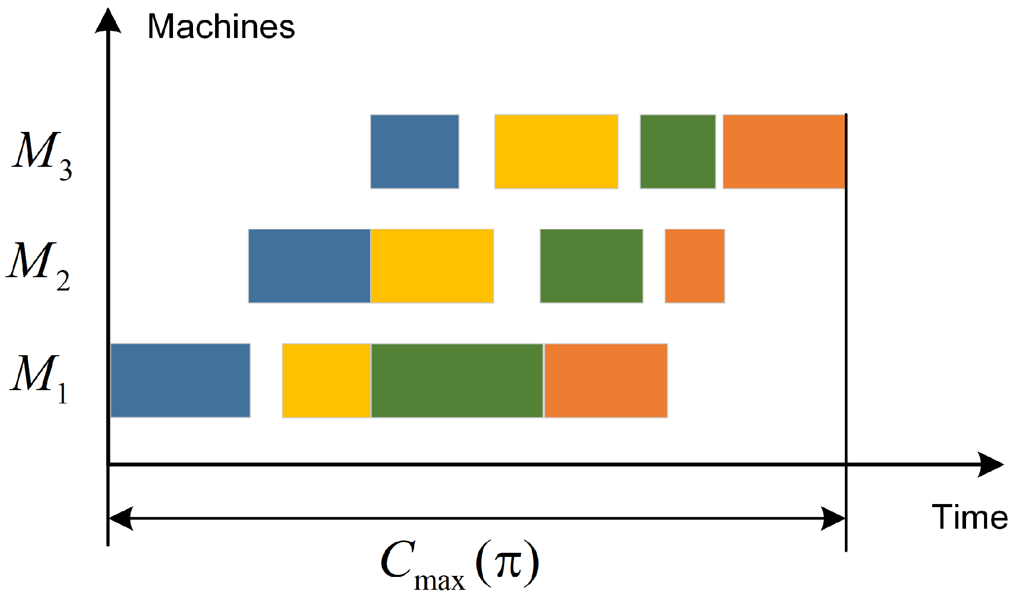
To provide a better understand of the problem formulation introduced above, the Gantt chart of a no-wait flow shop with three machines and four jobs is presented in Figure 1. As shown in the figure, the same color area indicates that the job is processed on different machines. Due to the no-wait constraint, the second job cannot be processed immediately after the first job is processed on the first machine.

2.2. Mathematical Formulation

This section introduces the mathematical formulation for the aforementioned problem. The parameters, decision variables, and specific models involved are as follows:

Parameters

M: Set of available machines.

N: Set of jobs to be processed.

m: Number of machines.

n: Number of jobs.

$p_{ij}$: Processing time of job j on machine i.

B: Upper value of makespan.

T: Upper value of total completion time.

Decision Variables

$x_{jk}$: Binary variable, $x_{jk}=1$ if job j is processed before job k, otherwise $x_{jk}=0$.

$C_{ij}$: Continuous variable, completion time of job j on machine i.

$S_{ij}$: Continuous variable, starting time of job j on machine i.

$TCT$: Continuous variable, the total completion time.

$C_{\max }$: Continuous variable, the completion time of the last job on the last machine.

Formally, the mathematical model of the NWFSP can be formulated as follows:

$$\min C_{\max }$$

(1)

subject to:

$$C_{\max }\ge C_{m,j},\forall j\in N$$

(2)

$$TCT=\sum _{i=1}^m{C}_{i,n},\forall i\in M$$

(3)

$$TCT\le T$$

(4)

$$x_{jk}+x_{kj}=1,\forall j,k\in N,j>k$$

(5)

$$x_{jk}+x_{kl}+x_{lj}\le 2,\forall j,k,l\in N,j\ne k\ne l$$

(6)

$$C_{ij}=S_{ij}+p_{ij},\forall j\in N,\forall i\in M$$

(7)

$$S_{ij}\ge C_{i-1,j},\forall j\in N,\forall i\in M\backslash \left\{1\right\}$$

(8)

$$S_{ij}\ge C_{ik}-B{x}_{jk},\forall i\in M,\forall j,k\in N,j>k$$

(9)

$$S_{ij}\ge C_{ij}-B(1-x_{jk}),\forall i\in M,\forall j,k\in N,j>k$$

(10)

$$x_{jk}\in \{0,1\},\forall j,k\in N,j\ne k$$

(11)

$$S_{ij}\ge 0,C_{ij}\ge 0,\forall j\in N,\forall i\in M$$

(12)

where the objective of the problem is to minimize the makespan. Equations (2) and (3) are the definition formulas of makespan and total completion time. Equation (4) represents a total completion time constraint, where T is a value determined by the scheduler. Equation (5) represents the processing order constraint of any two jobs. Equation (6) ensures that the processing sequence of any jobs will not be contradictory. Equation (7) gives the relationship between the start time and the completion time of the job. Equation (8) guarantees no-wait constraint for the job to be processed on two consecutive machines. Equations (9) and (10) represent the constraint relationship of the start and completion time under the order of different jobs.

2.3. Interval-Valued Fuzzy Set

An interval-valued fuzzy set $\tilde{A}$ in $X\in (-\infty ,+\infty )$ is defined as

$$\tilde{A}=\left\{\left(x,\left[{\mu }_{A^U}\left(x\right),{\mu }_{A^L}\left(x\right)\right]\right)\right\},x\in X$$

where $0\le {\mu }_{A^L}\left(x\right)\le {\mu }_{A^U}\left(x\right)\le 1$ are the membership functions (MFs), x is the set of real numbers. Symbolically, $\tilde{A}$ is denoted by $\tilde{A}=\left(\begin{array}{c}{A}^U\\ A^L\end{array}\right)$, $A^U$ and $A^L$ are trapezoidal fuzzy sets defined on upper and lower MFs, respectively.

Example 1.

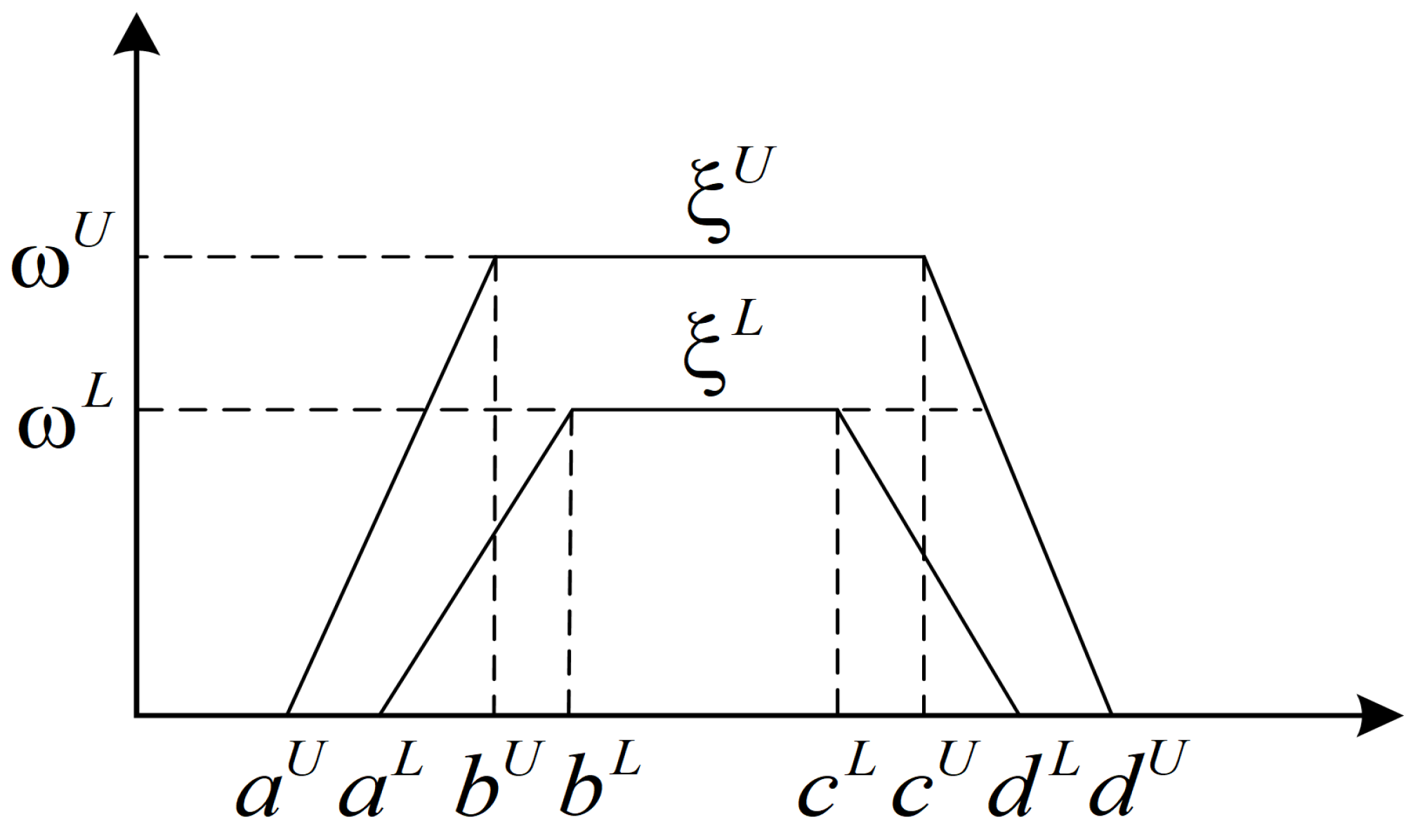
An interval-valued trapezoidal fuzzy variable $\tilde{\xi }$ of IVFSs determined by

$$\tilde{\xi }=\left(\begin{array}{c}{\xi }^U\\ {\xi }^L\end{array}\right)=\left(\begin{array}{c}{a}^U,b^U,c^U,d^U;{\omega }_{}^U\\ a^L,b^L,c^L,d^L;{\omega }_{}^L\end{array}\right)$$

where the levels $0\le {\omega }^L,{\omega }^U\le 1$, and ${\omega }^U$, ${\omega }^L$ are the height of trapezoidal fuzzy variables ${\xi }^U$, ${\xi }^L$, respectively. Specially, if ${\omega }^U=1,{\omega }^L=1$, the ${\xi }^U,{\xi }^L$ are normalized. The upper and lower fuzzy numbers of $\tilde{\xi }$ are shown in Figure 2.

To consider the uncertainties of the job processing times in practical applications, the processing times are described as interval-value fuzzy numbers. According to Example 1, the uncertain processing times $\widetilde{p_{ij}}$ of job j on machine i are denoted as follows:

$$\widetilde{p_{ij}}=\left(\begin{array}{c}{p}_{ij}^U\\ p_{ij}^L\end{array}\right)=\left(\begin{array}{c}{p}_{ij,1}^U,p_{ij,2}^U,p_{ij,3}^U,p_{ij,4}^U;{\omega }_{ij}^U\\ p_{ij,1}^L,p_{ij,2}^L,p_{ij,3}^L,p_{ij,4}^L;{\omega }_{ij}^L\end{array}\right),i\in M,j\in N$$

(13)

where $p_{ij}^U$ and $p_{ij}^L$ are trapezoidal fuzzy variables defined on upper and lower MFs, ${\omega }_{ij}^U$ and ${\omega }_{ij}^L$ are the height of $p_{ij}^U$ and $p_{ij}^L$. Moreover, $p_{ij,1}^U$, $p_{ij,2}^U$, $p_{ij,1}^L$, and $p_{ij,2}^L$ are most optimistic values, $p_{ij,3}^U$, $p_{ij,4}^U$ $p_{ij,3}^L$, and $p_{ij,4}^L$ are most pessimistic values. The $p_{ij,1}^U$, $p_{ij,2}^U$, $p_{ij,3}^U$, $p_{ij,4}^U$, and $p_{ij,1}^L$, $p_{ij,2}^L$, $p_{ij,3}^L$, $p_{ij,4}^L$ are given as the ratios to the most likely processing times $p_{ij}$, ${\omega }_{ij}^U$, and ${\omega }_{ij}^L$ are randomly assigned values from $[0,1]$, respectively.

Although the NWFSP with uncertain processing times is considered. However, it is very complicated to deal with the scheduling problem with uncertain parameters. Therefore, in the next section, we will simplify this fuzzy programming model.

2.4. Robust NWFSP under Moment Uncertainty

In the following, a deterministic R-NWFSP model is suggested with the case of uncertain job processing times. There are some feasible approaches that can be used to deal with constrained optimization problems with uncertain parameters in scheduling. However, the chance-constrained programming [34] has been developed to solve these problems and proved to be one of the most effective methods. In the approach, the fuzzy constraint should be maintained under the assumption of predetermined credibility level to achieve the appropriate safety margin provided. For the upper and lower bounds of IVFSs that reflect the uncertain processing time of the job, two CCP models based on the credibility measure [11] are proposed for the R-NWFSP.

For the upper MF $(p_{ij,1}^U,p_{ij,2}^U,p_{ij,3}^U,p_{ij,4}^U;{\omega }_{ij}^U)$, the CCP model for the R-NWFSP related to processing time can be formulated as:

$$\left\{\begin{array}{c}\min C_{\max }^U\hfill \\ \mathrm{s}.\mathrm{t}. \mathrm{Cr}\left\{p_{ij}^U\le P_{ij}^U\right\}\ge {\alpha }^U\hfill \end{array}\right.$$

(14)

For the lower MF $(p_{ij,1}^L,p_{ij,2}^L,p_{ij,3}^L,p_{ij,4}^L;{\omega }_{ij}^L)$, the CCP model for the R-NWFSP related to processing time can be formulated as:

$$\left\{\begin{array}{c}\min C_{\max }^L\hfill \\ \mathrm{s}.\mathrm{t}. \mathrm{Cr}\left\{p_{ij}^L\le P_{ij}^L\right\}\ge {\alpha }^L\hfill \end{array}\right.$$

(15)

where ${\alpha }^U$ and ${\alpha }^L$ are the predetermined credibility levels, the abbreviation Cr represents chance, $P_{ij}^U$ and $P_{ij}^L$ are realization values that replace $C_{ij}^U-C_{i-1,j}^U$ and $C_{ij}^L-C_{i-1,j}^L$. Accordingly, after the determination, the decision maker will be sure that the actual realization of $p_{ij}^U$ and $p_{ij}^L$ will not be greater than $P_{ij}^U$ and $P_{ij}^L$, and their credibility are at least equal to ${\alpha }^U$ and ${\alpha }^L$.

Theorem 1.

If $\xi =(a,b,c,d;\omega )$ is a trapezoidal fuzzy variable with $a<b\le c<d$, the level $0<\omega \le 1$ and the predetermined credibility level $0<\alpha \le 1$, then $\mathrm{Cr}\{\xi \le x\}\ge \alpha$ is given as follows [25]:

$$\mathrm{Cr}\{\xi \le x\}\ge \alpha \Rightarrow \left\{\begin{array}{c}\frac{\left(\right(\omega -2\alpha )a+2\alpha b)}{\omega }\le x,if \alpha \le \frac{\omega }{2}\\ \frac{\left(2\right(\omega -\alpha )c+(2\alpha -\omega \left)d\right)}{\omega }\le x,if \alpha >\frac{\omega }{2}\end{array}\right.$$

(16)

where ω is called the height of ξ.

Corollary 1.

If $\xi =(a,b,c,d;\omega )$ is a trapezoidal fuzzy variable with $a<b\le c<d$, the level $0<\omega \le 1$ and the predetermined credibility level $0<\alpha \le 1$, then $\mathrm{Cr}\{\xi \ge x\}\ge \alpha$ is given as follows [25]:

$$\mathrm{Cr}\{\xi \ge x\}\ge \alpha \Rightarrow \left\{\begin{array}{c}\frac{\left(\right(\omega -2\alpha )d+2\alpha c)}{\omega }\ge x,if \alpha \le \frac{\omega }{2}\\ \frac{\left(2\right(\omega -\alpha )b+(2\alpha -\omega \left)a\right)}{\omega }\ge x,if \alpha >\frac{\omega }{2}\end{array}\right.$$

(17)

According to Theorem 1, for the interval-valued fuzzy processing time using credibility, we can do the following deterministic transformation of constraints:

$$\left\{\begin{array}{c}\mathrm{Cr}\left\{p_{ij}^U\le P_{ij}^U\right\}\ge {\alpha }^U\Rightarrow h_{ij}^U\le P_{ij}^U\\ \mathrm{Cr}\left\{p_{ij}^L\le P_{ij}^L\right\}\ge {\alpha }^L\Rightarrow h_{ij}^L\le P_{ij}^L\end{array}\right.$$

(18)

where

$$h_{ij}^U=\left\{\begin{array}{c}\frac{(({\omega }_{ij}^U-2{\alpha }^U)p_{ij,1}^U+2{\alpha }^U{p}_{ij,2}^U)}{{\omega }_{ij}^U},{\alpha }^U\le \frac{{\omega }_{ij}^U}{2}\\ \frac{(2({\omega }_{ij}^U-{\alpha }^U)p_{ij,3}^U+(2{\alpha }^U-{\omega }_{ij}^U)p_{ij,4}^U)}{{\omega }_{ij}^U},{\alpha }^U>\frac{{\omega }_{ij}^U}{2}\end{array}\right.$$

(19)

$$h_{ij}^L=\left\{\begin{array}{c}\frac{(({\omega }_{ij}^L-2{\alpha }^L)p_{ij,1}^L+2{\alpha }^L{p}_{ij,2}^L)}{{\omega }_{ij}^L},{\alpha }^L\le \frac{{\omega }_{ij}^L}{2}\\ \frac{(2({\omega }_{ij}^L-{\alpha }^L)p_{ij,3}^L+(2{\alpha }^L-{\omega }_{ij}^L)p_{ij,4}^L)}{{\omega }_{ij}^L},{\alpha }^L>\frac{{\omega }_{ij}^L}{2}\end{array}\right.$$

(20)

The corresponding deterministic models transformed into the models (14) and (15) have following equivalent expression:

$$\min {\tilde{C}}_{\max }^U$$

(21)

$$\min {\tilde{C}}_{\max }^L$$

(22)

where ${\tilde{C}}_{ij}^U=S_{ij}+h_{ij}^U$, ${\tilde{C}}_{ij}^L=S_{ij}+h_{ij}^L$.

Finally, the R-NWFSP model using linear weighted method has the following expression:

$$\min {\tilde{C}}_{\max }=\frac{1}{2}({\tilde{C}}_{\max }^U+{\tilde{C}}_{\max }^L)$$

(23)

As we transform the uncertain NWFSP into a equivalent deterministic model, the method of solving this problem can be simplified to the greatest extent. By designing a suitable solution algorithm, the biggest benefit is that it can be more convenient to achieve effective solutions. In the next section, we will design an intuitive solution method to solve the problem efficiently.

3. Solution Method

To solve the robust NWFSP under the proposed deterministic model, we next design an effective simulated annealing algorithm (SAA). The overall structure of the SAA for the R-NWFSP includes the following three phases: a NEH algorithm to generate the initial schedule, a neighborhood search to deeply improve the current sequence, and a new probability-based adaptive acceptance strategy and stop criteria.

3.1. Initial Solution

The NEH [35] is the most effective constructive heuristic algorithm, which has been proved to be the most efficient heuristic for PFSP [36]. Meanwhile, the main idea of this heuristic algorithm is also suitable for solving the no-wait flow shop scheduling problem. To efficiently find better schedule sequence, a NEH algorithm with the same priorities is applied to generate a better initial schedule.

Step 1: The same priorities of the NEH are used to sort all jobs in the non-ascending order of the total fuzzy processing time.

Step 2: Select the first two jobs and evaluate the possible ordering. The sequence with the smaller makespan will be taken as the current sequence.

Step 3: Put the following jobs one by one in all possible positions at the position with the smallest makespan as the current sub-sequence, until all jobs are inserted, to generate a complete job sequence.

3.2. Neighborhood Search

After the initial sequence is obtained, the SAA begins to iterate to find more feasible solutions. The selection of multiple neighborhood operators is of great importance to the performance of the designed SAA. Therefore, a variable neighborhood search (VNS) method is applied to find more feasible sequences, which contain swap, reversion, and insertion.

3.2.1. Swap

Note that $\pi =\{{\pi }_1,\dots ,{\pi }_l,\dots ,{\pi }_m,\dots ,{\pi }_n\}$ is a sequence of all jobs. The swap operator is applied to randomly select two jobs in the corresponding sequence, such as ${\pi }_l$, ${\pi }_m$, and to exchange the processing order of the two jobs to form a new one. Thus, the processing sequence is $\pi =\{{\pi }_1,\dots ,{\pi }_m,\dots ,{\pi }_l,\dots ,{\pi }_n\}$, as shown in Figure 3.

3.2.2. Reversion

Note that $\pi =\{{\pi }_1,\dots ,{\pi }_m,{\pi }_{m+1},\dots ,{\pi }_{m+l},\dots ,{\pi }_n\}$ is a sequence of all jobs. The reversion operator is applied to randomly select a processing sequence for reverse order operation, such as $\pi =\{{\pi }_1,\dots ,{\pi }_{m+l},{\pi }_{m+l-1},\dots ,{\pi }_m,\dots ,{\pi }_n\}$, as depicted in Figure 4.

3.2.3. Insertion

Note that $\pi =\{{\pi }_1,\dots ,{\pi }_l,\dots ,{\pi }_m,\dots ,{\pi }_n\}$ is a sequence of all jobs. The insertion operator is applied to randomly select one of the jobs from $\pi$, and to insert it at the front of another position, then $\pi =\{{\pi }_1,\dots ,{\pi }_m,{\pi }_l,\dots ,{\pi }_n\}$, as shown in Figure 5.

3.3. Acceptance and Stop Criteria

When the neighborhood search is generated, it is necessary to decide whether the newly generated sequence ${\pi }^{\prime }$ can be substituted into the next iteration. The Metropolis acceptance criterion [37] is the most important part of the simulated annealing, which allows accepting a slightly worse solution to take into account both global search and local optimization. Specifically, after the current sequence completes the neighborhood search in a given problem instance, the new generated ${\pi }^{\prime }$ is accepted with probability p as the incumbent schedule for the next iteration. This probability p is defined as follows:

$$p=min\left\{exp(\frac{C_{max}\left(\pi \right)-C_{max}\left({\pi }^{\prime }\right)}{T},1)\right\},$$

where T is a parameter that controls the annealing temperature and gradually decreases with the execution of the algorithm. In the context of different calculation examples, this temperature parameter T setting is different. According to the above formulas $(C_{max}\left(\pi \right)-C_{max}\left({\pi }^{\prime }\right))/T$, the longer the makespan, the higher the corresponding temperature parameter. Following the suggestions of Osman and Potts [38], the temperature is set as follows:

$$T=T_0·\frac{{\sum }_{j=1}^n{\sum }_{i=1}^m{h}_{ij}}{10·m·n},$$

where $T_0$ is a parameter to be adjusted, the parameter of temperature is set at $T_0=0.5$, and the termination temperature is set at $T=1$.

In order to facilitate the performance comparison with other algorithms, the maximum computational time $t_{max}$ as the running termination condition. The recommended SAA stops when the maximum computational time is reached. The schedule finally found can be considered as the optimal sequence in all iterative search processes.

3.4. Algorithm Framework

The simulated annealing algorithm is a very simple and effective meta-heuristic for solving various types of scheduling problems. In order to adapt simulated annealing algorithms to solve our problem efficiently, we firstly adopt the NEH algorithm to generate a better initial sequence. Then, a powerful neighborhood search method is applied to have better quality schedules. Related neighborhood search strategies are discussed in Section 3.2. Finally, a new acceptance strategy is designed to determine whether to accept the new sequence as the incumbent solution. Based on the settings of these important components, the SAA is designed to tackle the uncertain NWFSP efficiently. The complete framework of the SAA is presented in Algorithm 1.

Algorithm 1: Simulated Annealing Algorithm (SAA)

1 (Initial solution): Generate an initial schedule using the NEH algorithm;

2 Set the temperature $T=T_0\times {\displaystyle \sum _{j=1}^n\sum _{i=1}^m{h}_{ij}}/10\times n\times m$

3 Set initial iteration $in=0$;

4 Set maximum number of inner iterations $Inmax$;

5While the termination condition is not met do

6While $in\le Inmax$ do

7 Update iteration: $in\leftarrow in+1$

8 (Neighborhood search): Use the neighborhood search method that hybridizes the swap, reversion, and insertion to improve sequence ${\pi }^{\prime }$ in the previous step.

9 (Acceptance): Set $\pi ={\pi }^{\prime }$ with the probability of

10$p=\left\{\begin{array}{c}1,if \Delta <0\hfill \\ e^{-\Delta /T},if \Delta \ge 0\hfill \end{array}\right.$

11 where $\Delta =C_{\max }\left({\pi }^{\prime }\right)-C_{\max }\left(\pi \right)$.

12end While

13end While

14Output: The best solution found.

4. Numerical Experiments

4.1. Experimental Setup

To evaluate the experimental performance of SAA and R-NWFSP model, the developed algorithm for the R-NWFSP was coded using MATLAB. The simulation experiments were executed on a personal computer (PC) with an Intel(R) Core (TM) i5-4210 CPU @2.6 GHz and 16 GB RAM in a Windows 10 Operating System. It should be noted that the effectiveness of the algorithm is greatly affected by the number of different machines and jobs, and different data sets have been considered for parameter calibration and algorithm evaluation. To evaluate the performance of our designed algorithm with other approaches on different problem sizes, we used Taillard’s [39] problem scale to randomly generate 12 combined instances with different sizes n and m, where $n\in \{20,50,100,200,500\}$ and $m\in \{5,10,20\}$. For each scenarios, we carried out 10 independent replications for the designed SAA. The same stopping criterion applies to all comparison algorithms [40], but the criterion varies depending on the number of different machines and jobs. Specifically, the termination condition is set to the maximum running time $t_{max}=n^2$ ms.

The objective function is to minimize makespan under the constraint that TCT is less than or equal to a given value. For a given problem, the upper bound value T for the TCT is usually given by the scheduler. However, it is necessary to know that a very large T value used for computational experiments means that there are almost no constrains. On the other hand, a very small T value means that there is no feasible solution. Therefore, a valid T value should be chosen as the calculation experiment constraint. In this work, the total completion time of NEH initialization has been selected as the T value.

Table 1. Summary of test data.

Factors	Value
Number of jobs (n)	20/50/100/200/500
Number of machines (m)	5/10/20
Processing time for each operation ($p_{ij}$)	[1,99]
TCT constraint value (T)	Value of NEH solution

summarizes the required test parameters of the manufacturing system. Moreover, the $p_{ij,1}^U$, $p_{ij,2}^U$, $p_{ij,3}^U$, $p_{ij,4}^U$ are given as the ratios 0.7, 0.9, 1.1, 1.3, and the $p_{ij,1}^L$, $p_{ij,2}^L$, $p_{ij,3}^L$, $p_{ij,4}^L$ are given as the ratios 0.8, 0.95, 1.05, 1.2 to the most likely processing times $p_{ij}$, ${\omega }_{ij}^U$, and ${\omega }_{ij}^L$ are randomly assigned values from $[0,1]$, respectively.

To test the effectiveness and robustness of our designed SAA and compare the experiments results with other three algorithms visually, the average relative percentage deviation (ARPD) is introduced to measure the average relative quality of the solutions. The APRD has the following formulation:

$$ARPD=\frac{1}{R}\sum _{r=1}^R\frac{C_r-C^{*}}{C^{*}}\times 100$$

In addition, the standard deviation (SD) is employed to measure how close the solution is to the average solutions. The SD is given by:

$$SD=\sqrt{\frac{1}{R}{\displaystyle \sum _{r=1}^R}{\left[\frac{C_r-C^{*}}{C^{*}}\times 100-ARPD\right]}^2}$$

where $C_r$ is the current solution executed by a compared algorithm to the r-th iteration ($r=1,2,\dots ,R$) on a given problem scenario, and $C^{*}$ is the best solution found so far. Obviously, the smaller the value of ARPD (SD), the better the performance of the algorithm.

4.2. Comparison with Other Algorithms

To demonstrate the effectiveness and efficiency of the designed SAA in finding better quality schedules. We compare the experimental results obtained by SAA with other results obtained by genetic algorithm (GA) [41], tabu search (TS) [42], and firefly algorithm (FA) [43]. These algorithms are common meta-heuristics for solving the scheduling problems. The predetermined credibility levels ${\alpha }^L$ and ${\alpha }^U$ are set to ${\alpha }^U={\alpha }^L=0.3$. The experimental results are summarized in

Table 2. Comparison of results obtained by four algorithms with different instances.

$\mathit{n}\times \mathit{m}$	GA		TS		FA		SAA
	ARPD	SD	ARPD	SD	ARPD	SD	ARPD	SD
20, 5	2.00	1805.1	3.50	4.42	1.00	1.01	0.00	0.00
20, 10	2.20	1.65	4.39	4.81	1.10	1.07	0.03	0.02
20, 20	2.14	2.07	4.45	3.95	1.14	1.20	0.00	0.00
50, 5	2.93	3.04	6.46	6.01	2.16	2.19	0.27	0.19
50, 10	2.21	2.65	5.25	5.27	1.54	1.23	0.16	0.09
50, 20	1.51	2.72	4.43	4.89	1.13	1.65	0.13	0.13
100, 5	3.95	4.07	8.35	8.02	4.01	3.83	0.84	0.40
100, 10	2.51	2.98	5.69	4.92	1.66	1.21	0.30	0.33
100, 20	2.02	3.11	4.21	4.11	1.42	1.56	0.25	0.27
200, 10	4.84	5.83	8.74	8.05	4.27	3.86	0.58	0.62
200, 20	2.47	3.74	6.32	6.23	2.05	2.11	0.45	0.57
500, 20	7.35	8.21	12.32	12.11	4.62	4.63	1.22	1.39
Average	3.21	3.48	6.36	6.06	2.11	2.13	0.35	0.33

and

Table 3. Comparison of results with a makespan criterion.

$\mathit{n}\times \mathit{m}$	GA		TS		FA		SAA
	Best	Mean	Best	Mean	Best	Mean	Best	Mean
20, 5	1778.3	1778.3	1778.3	1778.3	1778.3	1778.3	1778.3	1778.3
20, 10	2201.5	2303.7	2235.2	2363.2	2211.4	2363.4	2224.5	2331.2
20, 20	2658.5	2858.3	2674.3	2898.2	2736.7	2904.8	2703.5	2882.6
50, 5	3382.8	3428.9	3432.4	3504.3	3412.1	3503.6	3407.2	3488.6
50, 10	5043.2	5273.6	5173.6	5364.2	5120.4	5322.6	5100.2	5323.3
50, 20	6542.4	6793.3	6631.4	6923.4	6633.6	6921.7	6631.6	6882.9
100, 5	6738.2	7074.2	6926.7	7372.2	6831.8	7252.4	6821.2	7286.1
100, 10	8810.1	9143.5	8982.6	9431.6	9013.4	9433.8	8963.6	9393.5
100, 20	10,730.4	11950.4	11,432.6	12,651.7	11,341.4	12,763.7	10,865.8	12,473.7
200, 10	15,542.3	16,327.7	15,934.9	17,352.3	16,023.6	17,121.7	15,863.5	16,929.5
200, 20	20,842.1	21,536.3	21,163.5	22,316.4	21,545.8	22,383.4	21,342.5	22,237.8
500, 20	48,242.6	49,717.1	49,135.7	51,256.4	49,438.4	51,753.3	49,320.1	51,642.3

. In the table, we compare the their experimental results for the four approaches. It is worth noting that the result of executing multiple times on the same instance, the experimental results may be quite different due to the stochastic nature of the meta-heuristic. As the number of problem instances increases, this phenomenon will become more and more obvious.

Table 2 summarizes the computational results of GA, TS, FA, and SAA. It is observed from Table 2 that the total average of ARPD by the designed SAA is low in most test cases. For the credibility levels ${\alpha }^U={\alpha }^L=0.3$, the average total ARPD obtained by SAA is only 0.35, which is better than the corresponding values of 3.21, 6.36, and 2.11 obtained by GA, TS, and FA, respectively. In other words, on average, the designed SAA can outperform GA, TS, and FA in terms of solution quality. In addition, a similar analysis of the SD can be found that the value obtained by SAA is only 0.33, which is much smaller than the value 3.48, 6.06, and 2.13 obtained by GA, TS, and FA. As far as the robustness of the solution is concerned, it fully illustrates the effectiveness of the designed algorithm.

Table 3 shows the comparison results of the aforementioned algorithms. It is revealed from Table 3 that the SAA is superior to other algorithms, and the results have been discovered through the extensive problem instances. Through further investigation of the statistical data in the table, we can find that the objective function of optimal value and average value obtained by our algorithm also performs best in these algorithms. Especially, when solving large-scale instances, the optimal and average value of the SAA are much better than other three algorithms. When the number of machines is small, the optimization problem is relatively easy to solve, and there is little difference in the effect of the algorithm. However, when the number of machines increases, the difficulty of the solution increases significantly.

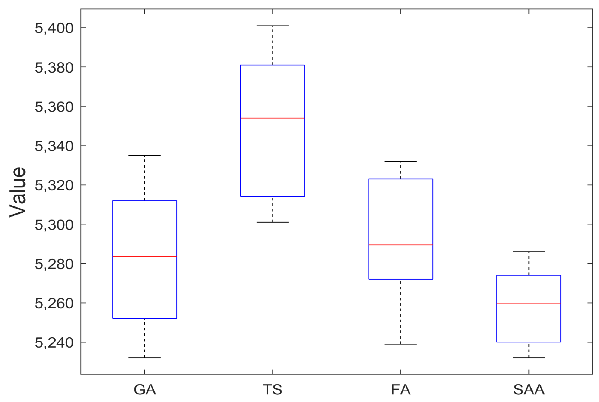
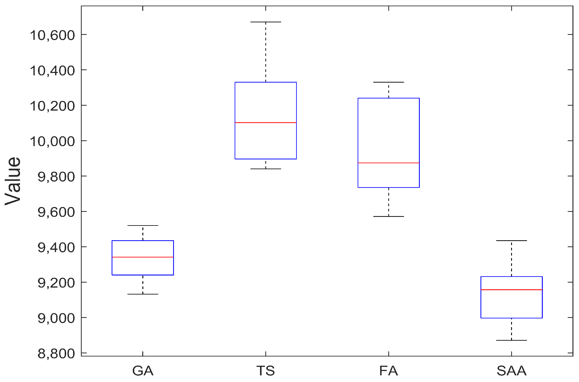
Figure 6 and Figure 7 illustrate the block diagrams of those approaches in the medium- and large-scale instances. It is obvious that the computational results obtained by the SAA is the smallest compared with the three corresponding comparison approaches, which fully proves that SAA has better performance. Since all tested algorithms are executed with the same stopping criterion in a similar computational environment, computational time consumption differs very little. Thus, we can conclude that the developed SAA performs well in terms of minimizing makespan from the best quality and average value of the algorithm execution.

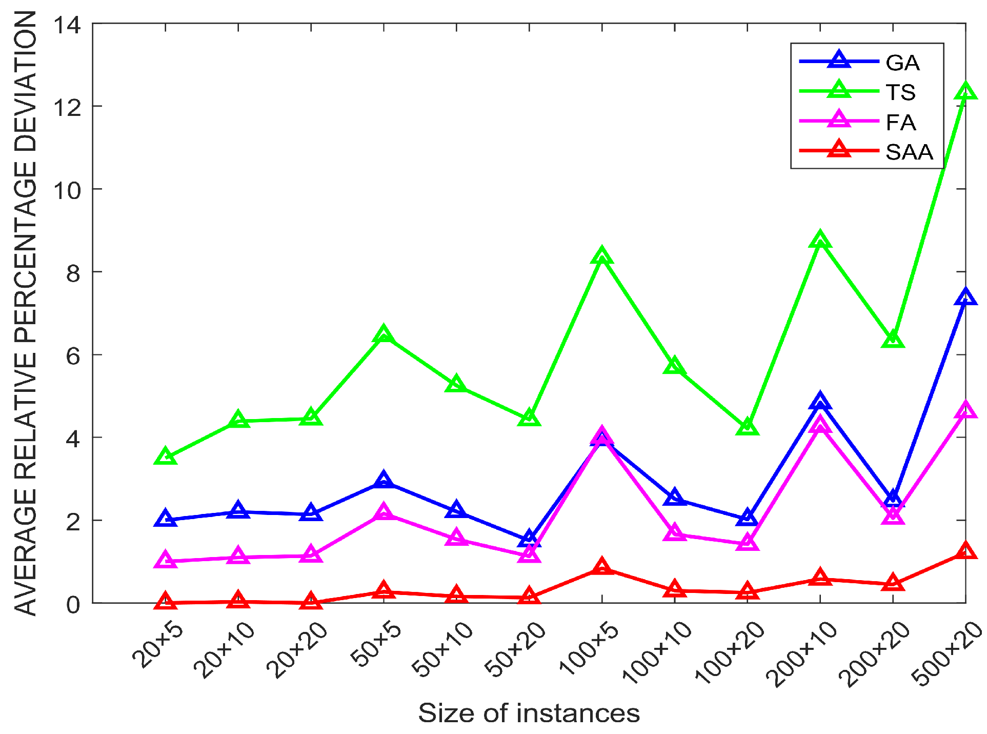
In order to compare the quality and diversity of the solution under different algorithms more intuitively, the average relative percentage deviation of different scale instances are drawn in Figure 8. This figure clearly illustrates that when the number of jobs and machines are small, the ARPD value is also small. As the size of the instance increases, the corresponding ARPD value gradually tends to increase. In addition, the value of ARPD is proportional to the number of jobs.

4.3. Sensitivity Analysis

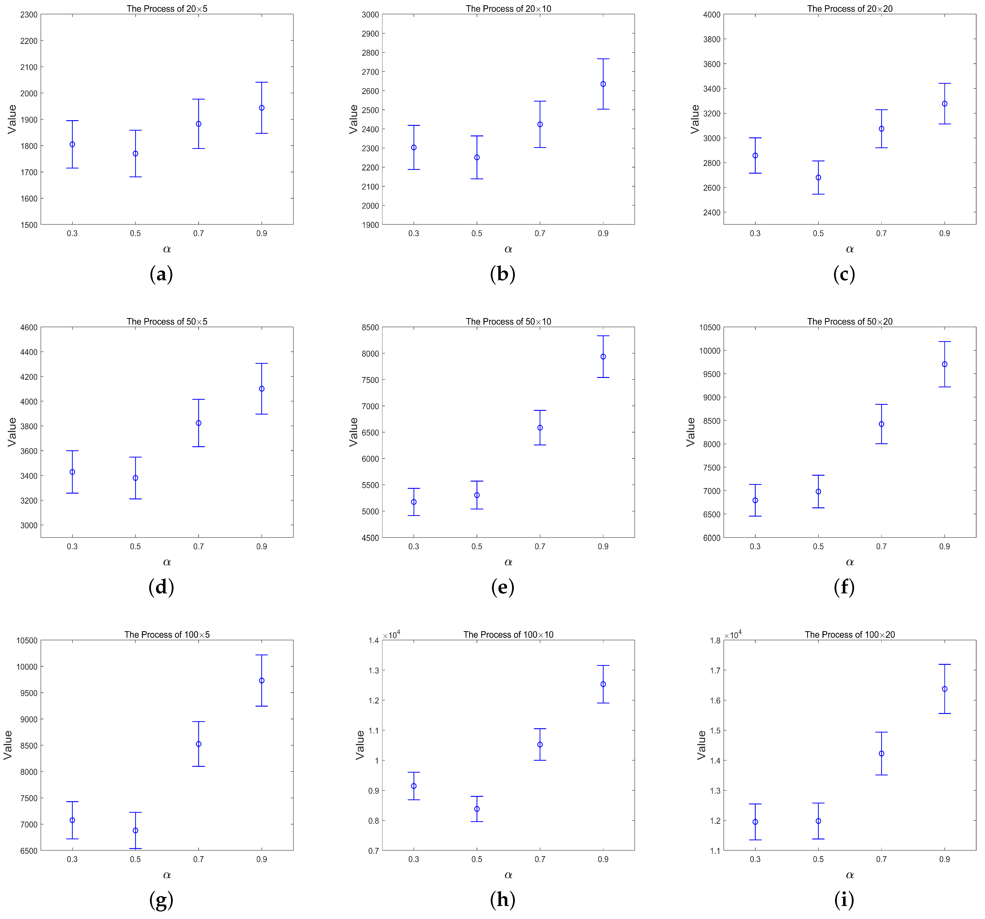
The previous analysis shows that the SAA for the R-NWFSP can outperform GA, TS, and FA. Therefore, in this subsection, SAA is adopted as a solution strategy to evaluate the performance of the proposed model under different credibility levels. We conducted a sensitivity analysis to evaluate the performance of R-NSFSP for the uncertain NWFSP under interval-valued fuzzy sets. For our experiments, the credibility level is selected from the set $\{0.3,0.5,0.7,0.9\}$, respectively. Obviously, according to (23), the optimal solution of the same instance varies with the credibility levels.

Figure 9 shows the experimental results for different credibility levels and different scales problems. These results indicate that different credibility levels of the model will affect the efficiency of SAA. For small-scale instances (a)–(c), experimental results show that the computational results under different confidence levels have small differences when $\alpha <0.5$. However, when $\alpha >0.5$ the makespan of this optimal solution increases as $\alpha$ increases.

For the medium- and large-scale instances (d)–(l), the computational results show that the best solutions of the model under different credibility levels are significantly different. It is observed from Figure 9 that when the credibility level is less than 0.5, the objective value under the optimal scheduling scheme is uncertain, indicating that the parameters have a greater impact on the model. When the credibility level is greater than 0.5, the objective value under the best solution has a positive relationship with the credibility levels. These results convincingly prove the excellent performance of the deterministic R-NWFSP model. Therefore, in practical applications, in order to minimize the impact of parameters on the model, it is recommended to set the credibility levels at 0.5 to achieve better performance. It should be noted that these explanations are almost very few exceptions because of the stochastic nature of meta-heuristic.

5. Conclusions

In this work, we discuss the uncertain no-wait flow shop scheduling problem (NWFSP) with the objective to minimize makespan under the constraint that the total completion time is not greater than a given bound. Firstly, due to the uncertainty of the job processing time in the practical applications, the processing times are regarded as the interval-valued fuzzy numbers. We propose a deterministic counterpart to optimal the robust NWFSP under the interval-valued fuzzy processing time, and an improved SAA is designed for its efficient solution. For the IVFSs using credibility, a chance constrained programming (CCP) is utilized to make the deterministic transformation of constraints. The corresponding deterministic model of the robust NWFSP is established. Then, in order to solve the certain linear programming efficiently, a SAA is specially designed. The SAA involves swap, insertion, reversion, and new acceptance criterion to find more promising solution. Finally, the designed approach is compared with GA, TS, and FA in instances with different sizes. Experimental results demonstrate that the designed approach has a better searching ability than other three algorithms for the robust NWFSP. Moreover, the applicability of the proposed model and solution method for the problem under interval-valued fuzzy sets is proved through a sensitivity analysis. Therefore, this work not only designs a solution method, but also provides a promising model transformation direction for uncertain scheduling problem with IVFSs.

Although our proposed model and solution strategy mainly solve the robust NWFSP, the study of this work is not limited to this. It can also be extended to many related fields of job assignment and sorting with uncertainties. In future work, it is meaningful to focus on the uncertainty and multi-objective attributes of the NWFSP, and develop more effective algorithms according to the characteristic of the problem to solve the realistic production scheduling problems.

References

1. Pinedo, M.L. Scheduling: Theory, Algorithms, and Systems, 4th ed.; Springer: New York, NY, USA, 2012. [Google Scholar]
2. Chien, C.-F.; Dauzère-Pérès, S.; Ehm, H.; Fowler, J.W.; Jiang, Z.; Krishnaswamy, S.; Lee, T.E.; Moench, L.; Uzsoy, R. Modelling and analysis of semiconductor manufacturing in a shrinking world: Challenges and successes. Eur. J. Ind. Eng. 2011, 5, 254–271. [Google Scholar] [CrossRef]
3. Huang, R.-H.; Yang, C.-L.; Huang, Y.-C. No-wait two-stage multiprocessor flow shop scheduling with unit setup. Int. J. Adv. Manuf. Technol. 2009, 44, 921–927. [Google Scholar] [CrossRef]
4. Nagano, M.S.; Da Silva, A.A.; Lorena, L.A.N. A new evolutionary clustering search for a no-wait flow shop problem with set-up times. Eng. Appl. Artif. Intell. 2012, 25, 1114–1120. [Google Scholar] [CrossRef]
5. Wang, Z.; Xing, W.; Bai, F. No-wait flexible flowshop scheduling with no-idle machines. Oper. Res. Lett. 2005, 33, 609–614. [Google Scholar] [CrossRef]
6. Agnetis, A. Scheduling no-wait robotic cells with two and three machines. Eur. J. Oper. Res. 2000, 123, 303–314. [Google Scholar] [CrossRef]
7. Shabtay, D. The just-in-time scheduling problem in a flow-shop scheduling system. Eur. J. Oper. Res. 2012, 216, 521–532. [Google Scholar] [CrossRef]
8. Allahverdi, A. A survey of scheduling problems with no-wait in process. Eur. J. Oper. Res. 2016, 255, 665–686. [Google Scholar] [CrossRef]
9. Schrijver, A. Combinatorial Optimization: Polyhedra and Efficiency, 1st ed.; Springer: Heidelberg, Germany, 2003. [Google Scholar]
10. Ding, J.-Y.; Song, S.; Gupta, J.N.D.; Zhang, R.; Chiong, R.; Wu, C. An improved iterated greedy algorithm with a Tabu-based reconstruction strategy for the no-wait flowshop scheduling problem. Appl. Soft Comput. 2015, 30, 604–613. [Google Scholar] [CrossRef]
11. Baoding, L.; Yian-Kui, L. Expected value of fuzzy variable and fuzzy expected value models. IEEE Trans. Fuzzy Syst. 2002, 10, 445–450. [Google Scholar] [CrossRef]
12. Röck, H. The Three-Machine No-Wait Flow Shop is NP-Complete. Assoc. Comput. Mach. 1984, 31, 336–345. [Google Scholar] [CrossRef]
13. Sahni, S.; Cho, Y. Complexity of Scheduling Shops with No Wait in Process. Math. Oper. Res. 1979, 4, 448–457. [Google Scholar] [CrossRef]
14. Pan, Q.-K.; Fatih, T.M.; Liang, Y.-C. A discrete particle swarm optimization algorithm for the no-wait flowshop scheduling problem. Comput. Oper. Res. 2008, 35, 2807–2839. [Google Scholar] [CrossRef]
15. Zhao, F.; Liu, H.; Zhang, Y.; Ma, W.; Zhang, C. A discrete Water Wave Optimization algorithm for no-wait flow shop scheduling problem. Expert Syst. Appl. 2018, 91, 347–363. [Google Scholar] [CrossRef]
16. Allahverdi, A.; Aydilek, H.; Aydilek, A. No-wait flowshop scheduling problem with two criteria; total tardiness and makespan. Eur. J. Oper. Res. 2018, 269, 590–601. [Google Scholar] [CrossRef]
17. Temİz, İ.; Erol, S. Fuzzy branch-and-bound algorithm for flow shop scheduling. J. Intell. Manuf. 2004, 15, 449–454. [Google Scholar] [CrossRef]
18. Han, Y.; Gong, D.; Jin, Y.; Pan, Q.-K. Evolutionary multi-objective blocking lot-streaming flow shop scheduling with interval processing time. Appl. Soft Comput. 2016, 42, 229–245. [Google Scholar] [CrossRef]
19. Daniels, R.L.; Kouvelis, P. Robust scheduling to hedge against processing time uncertainty in single-stage production. Manag. Sci. 1995, 41, 363–376. [Google Scholar] [CrossRef]
20. Zadeh, L.A. Fuzzy sets. Inf. Control 1965, 8, 338–353. [Google Scholar] [CrossRef] [Green Version]
21. Noori-Darvish, S.; Mahdavi, I.; Mahdavi-Amiri, N. A bi-objective possibilistic programming model for open shop scheduling problems with sequence-dependent setup times, fuzzy processing times, and fuzzy due dates. Appl. Soft Comput. 2012, 12, 1399–1416. [Google Scholar] [CrossRef]
22. Liu, G.-S.; Zhou, Y.; Yang, H.-D. Minimizing energy consumption and tardiness penalty for fuzzy flow shop scheduling with state-dependent setup time. J. Clean. Prod. 2017, 147, 470–484. [Google Scholar] [CrossRef]
23. Shao, Z.; Shao, W.; Pi, D. Effective heuristics and metaheuristics for the distributed fuzzy blocking flow-shop scheduling problem. Swarm Evol. Comput. 2020, 59, 100747. [Google Scholar] [CrossRef]
24. Long, J.; Sun, Z.; Pardalos, P.M.; Bai, Y.; Zhang, S.; Li, C. A robust dynamic scheduling approach based on release time series forecasting for the steelmaking-continuous casting production. Appl. Soft Comput. 2020, 92, 106271. [Google Scholar] [CrossRef]
25. Kundu, P.; Majumder, S.; Kar, S.; Maiti, M. A method to solve linear programming problem with interval type-2 fuzzy parameters. Fuzzy Optim. Decis. Mak. 2019, 18, 103–130. [Google Scholar] [CrossRef]
26. Lu, C.-C.; Lin, S.-W.; Ying, K.-C. Minimizing worst-case regret of makespan on a single machine with uncertain processing and setup times. Appl. Soft Comput. 2014, 23, 144–151. [Google Scholar] [CrossRef]
27. Ashtiani, B.; Haghighirad, F.; Makui, A.; Montazer, G.L. Extension of fuzzy TOPSIS method based on interval-valued fuzzy sets. Appl. Soft Comput. 2009, 9, 457–461. [Google Scholar] [CrossRef]
28. Allahverdi, A.; Aydilek, H.; Aydilek, A. Single machine scheduling problem with interval processing times to minimize mean weighted completion time. Comput. Oper. Res. 2014, 51, 200–207. [Google Scholar] [CrossRef]
29. Yao, J.-S.; Lin, F.-T. Constructing a fuzzy flow-shop sequencing model based on statistical data. Int. J. Approx. Reason. 2002, 29, 215–234. [Google Scholar] [CrossRef] [Green Version]
30. Aydilek, H.; Allahverdi, A. A polynomial time heuristic for the two-machine flowshop scheduling problem with setup times and random processing times. Appl. Math. Model. 2013, 37, 7164–7173. [Google Scholar] [CrossRef]
31. Pereira, J. The robust (minmax regret) single machine scheduling with interval processing times and total weighted completion time objective. Comput. Oper. Res. 2016, 66, 141–152. [Google Scholar] [CrossRef]
32. Dorfeshan, Y.; Tavakkoli-Moghaddam, R.; Mousavi, S.M.; Vahedi-Nouri, B. A new weighted distance-based approximation methodology for flow shop scheduling group decisions under the interval-valued fuzzy processing time. Appl. Soft Comput. 2020, 91, 106248. [Google Scholar] [CrossRef]
33. Gupta, J.N.D.; Stafford, E.F. Flowshop scheduling research after five decades. Eur. J. Oper. Res. 2006, 169, 699–711. [Google Scholar] [CrossRef]
34. Charnes, A.; Cooper, W.W. Chance-Constrained Programming. Manag. Sci. 1959, 6, 73–79. [Google Scholar] [CrossRef]
35. Nawaz, M.; Enscore, E.E.; Ham, I. A heuristic algorithm for the m-machine, n-job flow-shop sequencing problem. OMEGA 1983, 11, 91–95. [Google Scholar] [CrossRef]
36. Kalczynski, P.J.; Kamburowski, J. On the NEH heuristic for minimizing the makespan in permutation flow shops. OMEGA 2007, 35, 53–60. [Google Scholar] [CrossRef]
37. Metropolis, N.; Rosenbluth, A.W.; Rosenbluth, M.N.; Teller, A.H.; Teller, E. Equation of State by Fast Computing Machines. J. Chem. Phys. 1953, 21, 1087–1092. [Google Scholar] [CrossRef] [Green Version]
38. Osman, I.H.; Potts, C.N. Simulated annealing for permutation flow-shop scheduling. OMEGA 1989, 17, 551–557. [Google Scholar] [CrossRef]
39. Taillard, E. Benchmarks for basic scheduling problems. Eur. J. Oper. Res. 1993, 64, 278–285. [Google Scholar] [CrossRef]
40. Črepinšek, M.; Liu, S.-H.; Mernik, M. Replication and comparison of computational experiments in applied evolutionary computing: Common pitfalls and guidelines to avoid them. Appl. Soft Comput. 2014, 19, 161–170. [Google Scholar] [CrossRef]
41. Ahmadizar, F.; Zarei, A. Minimizing makespan in a group shop with fuzzy release dates and processing times. Int. J. Adv. Manuf. Technol. 2013, 66, 2063–2074. [Google Scholar] [CrossRef]
42. Ben-Daya, M.; Al-Fawzan, M. A tabu search approach for the flow shop scheduling problem. Eur. J. Oper. Res. 1998, 109, 88–95. [Google Scholar] [CrossRef]
43. Udaiyakumar, K.C.; Chandrasekaran, M. Application of Firefly Algorithm in Job Shop Scheduling Problem for Minimization of Makespan. Procedia Eng. 2014, 97, 1798–1807. [Google Scholar] [CrossRef] [Green Version]
Figure 1. A Gantt chart of a no-wait flow shop.
Processes 09 00789 g001
Figure 2. Interval-value fuzzy number.
Processes 09 00789 g002
Figure 3. Illustration of Swap operator.
Processes 09 00789 g003
Figure 4. Illustration of Reversion operator.
Processes 09 00789 g004
Figure 5. Illustration of Insertion operator.
Processes 09 00789 g005
Figure 6. Boxplot for the process of 50 × 10.
Processes 09 00789 g006
Figure 7. Boxplot for the process of 100 × 10.
Processes 09 00789 g007
Figure 8. Relation graph for different instances.
Processes 09 00789 g008
Figure 9. The value under different credibility levels. For small-scale instances (ac), experimental results show that the computational results under different confidence levels have small differences when α < 0.5. For the medium- and large-scale instances (dl), the computational results show that the best solutions of the model under different credibility levels are significantly different.
Processes 09 00789 g009aProcesses 09 00789 g009b