Abstract
A countershaft brake is used as a transmission brake (TB) to realize synchronous shifting by reducing the automated mechanical transmission (AMT) input shaft’s speed rapidly. This process is performed to reduce shifting time and improve shifting quality for heavy-duty vehicles equipped with AMT without synchronizer. To improve controlled synchronous shifting, the AMT input shaft’s equivalent resistance torque and the TB’s characteristic parameters are studied. An AMT dynamic model under neutral gear position is analyzed during the synchronous control interval. A dynamic model of the countershaft brake is discussed, and its control flow is given. The parameter identification method of the AMT input shaft’s equivalent resistance torque is given on the basis of the least squares algorithm. The parameter identification of the TB’s characteristic parameters is proposed on the basis of the recursive least squares method (RLSM). Experimental results show that the recursive estimations of the TB’s characteristic parameters under different duty cycles of the TB solenoid valve, including brake torque estimation, estimation accuracy, and braking intensity estimation, can be effectively estimated. The research provides some reliable evidence to further study the synchronous shifting control schedule for heavy-duty vehicles with AMT.
1. Introduction
Synchronizers are widely used in cars and light-duty vehicles to improve shifting quality and reduce shifting time [1,2]. However, they cannot be widely used in heavy-duty vehicles limited by manufacturing technology and the strength of materials [3,4,5]. Automated mechanical transmission (AMT) was developed on the basis of manual transmission equipped with automatic clutch and automatic choosing-shifting actuator [6,7]. In recent decades, AMT has been used in heavy-duty vehicles due to its great transmission torque, high transmission efficiency, low manufacturing costs, and low maintenance costs [8,9,10]. Currently, other types of automated transmissions such as automatic transmission (AT), continuously variable transmission (CVT), and double clutch transmission (DCT), still cannot meet the requirements of heavy-duty vehicles. AT has low transmission efficiency and high maintenance costs, thereby increasing operational costs [11,12,13]. CVT has low transmission torque limited by steel belt materials and manufacturing technology, and has been only used in cars [14,15,16]. DCT cannot provide sufficient transmission torque for heavy-duty vehicles owing to its complex mechanical structures and advanced manufacturing technologies [17,18,19].
AMT without synchronizer cannot achieve synchronous shifting and reduce shifting shock during shifting. The transmission brake (TB) was designed and produced for some AMT manufacturers to achieve synchronous shifting [20]. During upshifting, the AMT input shaft’s speed or the AMT countershaft’s speed should be rapidly decreased to meet the requirements of the transmission ratio between the AMT input shaft and the AMT output shaft for the new gear position. In practice, the brake characteristics of the TB can be influenced by environmental temperature, lubrication condition, and wear condition. The movements of the clutch actuator, choosing-shifting actuator, and TB actuator have some obvious lagging and nonlinear qualities, making it difficult to completely achieve synchronization at the shifting moment. Thus, a transmission control unit (TCU) needs to control the TB to make the AMT input shaft’s speed decelerate in accordance with the given speed curve.
In this paper, the AMT dynamic analysis is studied first when AMT is in neutral position. The TB dynamic analysis is then analyzed for synchronous shifting control. The estimation methods about the equivalent resistance torque of the AMT input shaft and the TB’s characteristic parameters are then studied. Finally, the parameter estimation is studied on the basis of the experimental data.
2. AMT Dynamic Analysis
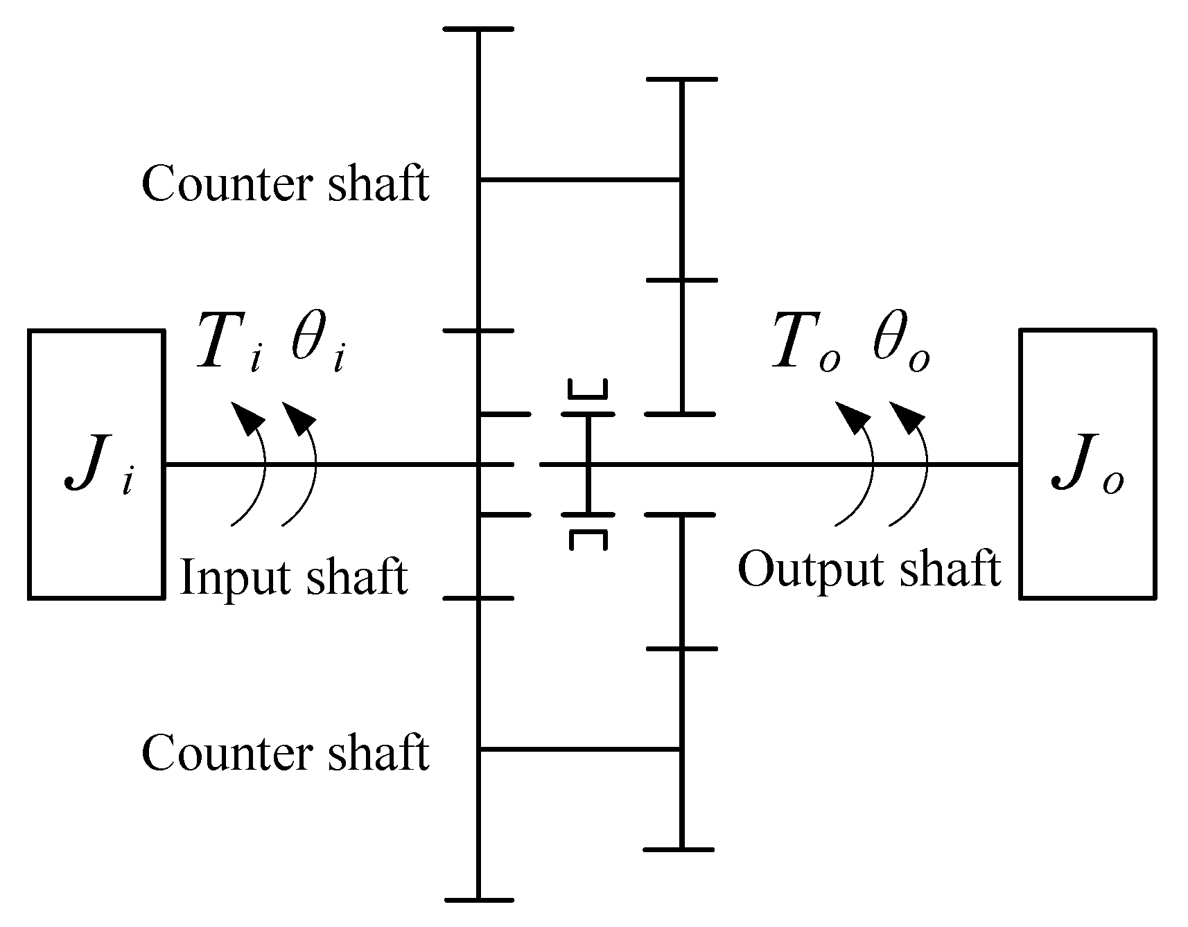
The clutch is disengaged and the gear is in neutral. The AMT dynamic model under neutral gear position is shown in Figure 1.

Figure 1.
AMT dynamic model under neutral gear position.
The dynamic equation of AMT dynamic model under neutral gear position can be expressed as Equation (1)
where is the mass matrix expressed as , is the velocity matrix expressed as , is damping matrix expressed as , and is force matrix expressed as .
The main parameters of Equation (1) are listed in Table 1.

Table 1.
Model parameters.
3. TB Analysis
3.1. TB Model
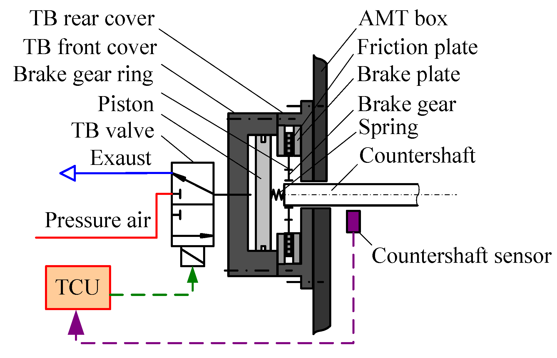
The AMT input shaft’s speed should be decreased owing to the low transmission ratio to shift from low gear position to high. The countershaft brake can be easily assembled and can achieve the function of reducing the AMT input shaft’s speed to meet the synchronization condition and reduce shifting time. Thus, the countershaft brake is used as the TB in a heavy-duty AMT. Figure 2 shows the schematic of the TB system.

Figure 2.
Schematic of the TB system.
The TB solenoid valve is a high speed, on–off, normally closed solenoid valve. Compressed air enters the TB through the solenoid valve when the TCU gives instruction to the TB solenoid valve. The piston moves towards the brake plate under the pressure of compressed air, and the brake torque is created when the brake plate and the friction plate are compressed. The inner engaging ring of the friction plate is engaged with the outer engaging gear of the brake gear, and the countershaft begins slowing down under the action of brake torque.
The force acting on the valve spool includes the force of the compressed air, electromagnetic force, spring force, friction force, and resistance force from the brake chamber. The movement of the valve spool can be expressed as Equation (2)
where is the displacement of the valve spool, is the moving velocity of the valve spool, is the force of the compressed air, is the electromagnetic fore, is the spring force, is the friction force of the valve spool moving, is the resistance force in the brake chamber, is the damping coefficient of the valve spool moving, and is the moving mass of the valve spool.
The movement of the cylinder can be expressed as Equation (3)
where is the piston displacement, is the piston mass, is the compressed gas acting force on the piston, is the gas acting force on the piston in the brake chamber, is the force of the cylinder spring, is the friction force of the piston moving, is the damping coefficient of the piston moving, and is the moving velocity of the piston.
TB torque is considered an equivalent brake torque at the AMT input shaft and can be expressed as Equation (4)
where is the TB torque, is the number of friction surfaces, is the area of the friction plate, is the equivalent radius of the friction plate, and is the transmission ratio between the input shaft and the countershaft.
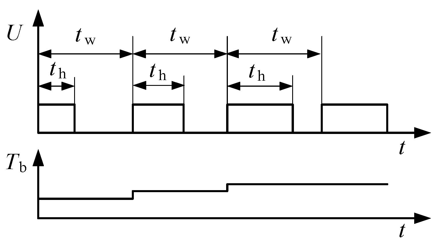
In practical operation, the duty cycle of the solenoid valve is used to control the flow of the TB solenoid valve. The duty cycle can be expressed as Equation (5)
where is the duty cycle, and and are the cycle time and high-level time of the solenoid valve, respectively.
The angular deceleration of the AMT input shaft can be controlled by controlling the pulse width modulation. The relationship between the flow of the TB solenoid valve and the duty cycle is approximately linear [21]. In particularly, the mean brake torque can be regulated by regulating the duty cycle of the TB solenoid valve. The mean brake torque can be increased by increasing the duty cycle of the TB solenoid valve, as shown in Figure 3.

Figure 3.
Relationship between the mean brake torque and the duty cycle.
The brake characteristics have some complexities owing to the nonlinear performance of the solenoid valve spool and the brake piston. The dynamic response time of opening or closing the solenoid valve is approximately 2 ms [22,23]. This phenomenon is caused by the lag times of the electric current and the valve spool movement. The lag time of TB action becomes longer if the duty cycle is smaller.
3.2. Synchronous Shifting Condition
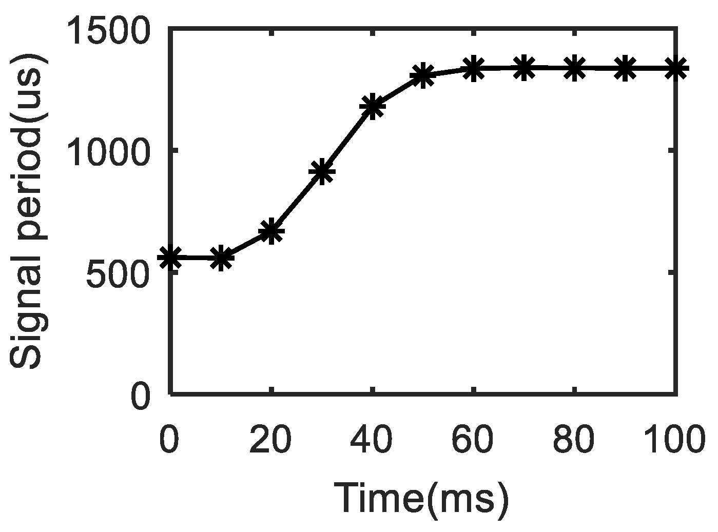
Figure 4 shows the signal period curve of the choosing actuator from one neutral gear position to another neutral gear position. This curve is approximately 60 ms between the two adjacent neutral gear positions. Thus, the operation of choosing gear position and the synchronous shifting control can be conducted simultaneously when the completion time of braking the AMT input shaft is longer than that of choosing gear position.
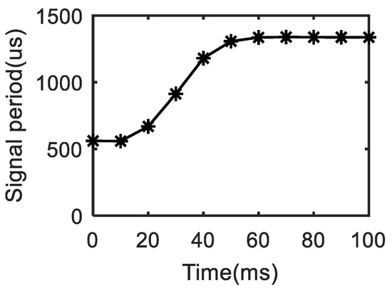
Figure 4.
Signal period between the two adjacent neutral gear positions.
The angular deceleration of the AMT output shaft when in the neutral position changes because the load mass and the running resistance torque vary in wide ranges for heavy-duty vehicles. The loss of the AMT input shaft’s speed is generated from the time of the shifting command given by the TCU to the time of engaging the new gear position because relieving the TB and shifting gear have lag performance. Considering this lag performance, the synchronous speed difference condition is designed as the judgement of shifting moment.
The synchronous speed difference condition during the upshifting process is expressed as Equation (6)
where is the value of the needed synchronous speed difference.
If is a short interval time from the time of the shifting command given by the TCU to the time of contacting the engaging gears for the new gear position, is the number of the current gear position, is the transmission ratio of the new gear position, and and are the losses of the AMT input shaft’s speed and the AMT output shaft’s speed, respectively. The value of the synchronous speed difference for upshifting to the new gear position can then be calculated from Equation (7)
Equation (7) indicates that the value of the synchronous speed difference decreases with the increase in the running resistance torque under the conditions of the same gear position and same loads. Specially, the running resistance torque increases and the value of the synchronous speed difference decreases if heavy-duty vehicles run on the road with a large slope. This condition also indicates that the value of the synchronous speed difference increases with a decrease of the transmission ratio under the conditions of the same gear position and same loads. In particular, the value of the synchronous speed difference increases if the AMT is shifted to a higher gear position.
3.3. TB Control Flow
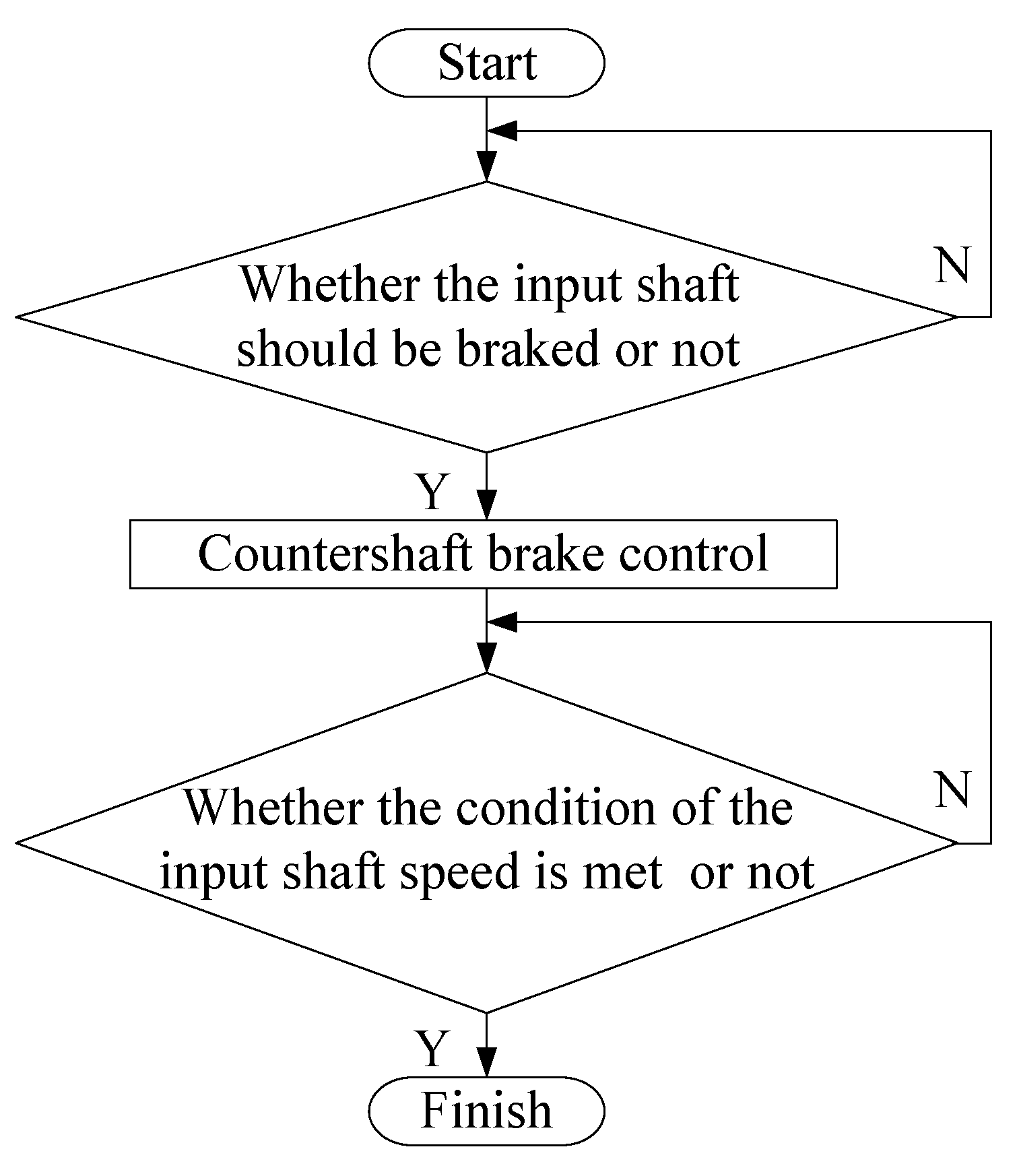
The logical diagram of the TB control program for heavy-duty vehicles is shown in Figure 5. The TB control program is started if the AMT input shaft needs to be decelerated rapidly. The TB control program is stopped if the input shaft can meet the requirements of the synchronous upshifting condition which is expressed in Equation (6).
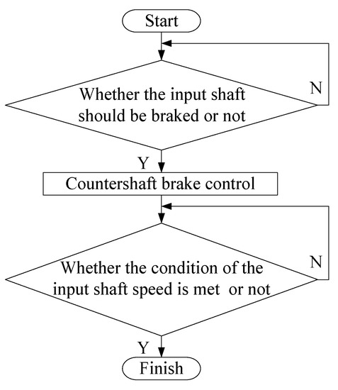
Figure 5.
Logical diagram of TB control flow.
4. Estimation Method of TB Characteristic Parameters
The equivalent running resistance torque of the AMT input shaft is derived from the frictions, including bearings, splines, and gears. Therefore, the equivalent running resistance torque needs to be estimated for the purpose of precise synchronous upshifting control. The estimation method of the brake torque and other brake characteristic parameters should be studied to control the deceleration process of the AMT input shaft using the TB precisely.
4.1. Estimation Method of AMT Equivalent Resistance Torque
4.1.1. A. Estimation Algorithm
After cutting power through clutch disengaging and putting the gear position in neutral, the AMT input shaft’s speed decreases due to inertia and resistance torque. The discrete dynamic equation of the AMT input shaft under this condition can be expressed as Equation (8)
where is the sampling interval is the AMT input shaft’s angular acceleration at No. k sampling time, , and are the AMT input shaft’s angular speeds at No. k sampling time and No. (k − 1) sampling time, respectively. is the rotational torque of the AMT input shaft at No. k sampling time, ,, and are the friction torques caused by bearings, engaging gears, and engaging splines at No. k sampling time, respectively.
Supposing the resistance torque cannot change with the AMT input shaft’s speed by ignoring the influence of system damping, the AMT input shaft’s angular speed can be expressed as Equation (9)
where is the time, and and are the AMT input shaft’s angular speed and the AMT input shaft’s angular acceleration under the conditions of clutch disengaging and neutral gear position.
The sum square of measurement errors can be expressed as Equation (10)
where is the time at No. k sampling time.
Using the least squares fitting method and marking and as the estimation values of and separately, taking the derivative of Equation (10) with respect to and and letting them be equal to zero, the expression is given as Equation (11)
and can be calculated from Equation (11). , which is marked as the equivalent resistance torque estimation of the AMT input shaft, can be obtained. The estimation algorithm about the equivalent resistance torque of the AMT input shaft can be expressed as Equation (12)
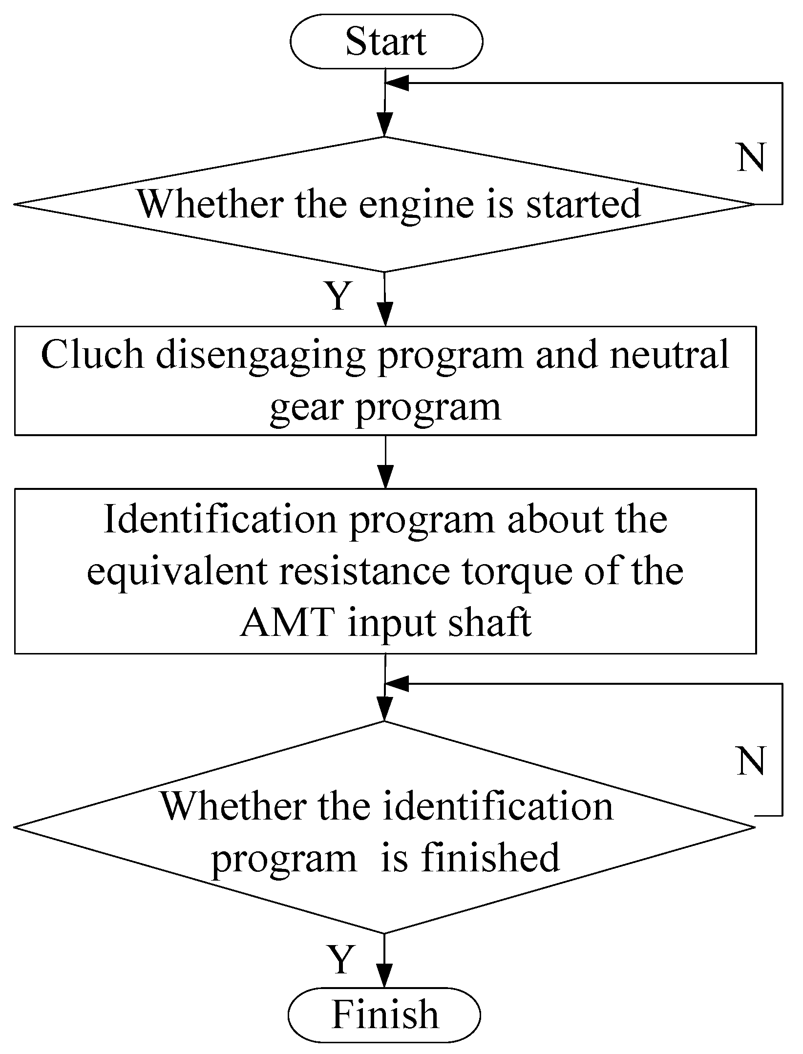
4.1.2. Flow of Identification Process
The identification process about the equivalent resistance torque of the AMT input shaft should be completed before starting the vehicle. Figure 6 gives the identification process and the completion condition where the AMT input shaft’s speed decreases to engine idle speed.
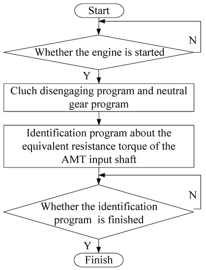
Figure 6.
Flow of identification about the equivalent resistance torque of the input shaft.
4.2. Estimation Method of TB Torque
The observation model about the brake torque should be given firstly to estimate the TB torque. The brake torque can then be identified on the basis of the RLSM.
4.2.1. Observation Model of TB Torque
The dynamic equation of the AMT input shaft can be expressed as Equation (13) in accordance with Equation (1) if TB is used
Replacing the equivalent resistance torque of the AMT input shaft with the equivalent resistance torque estimation, the discrete dynamic equation of the AMT input shaft, according to Equation (13), can be expressed as Equation (14)
Ignoring the influence of system damping and considering the measurement error, the observation equation of TB torque at No. k sampling time can be expressed as Equation (15)
where is the observation value expressed as , is the gain expressed as , and and are the estimation values of TB torque and measurement error at No. k sampling time, respectively.
Therefore, the observation model about the estimated parameter is given as Equation (16)
where is the observation matrix expressed as , is the gain matrix expressed as , is the measurement error matrix expressed as , and is the estimation value matrix expressed as .
4.2.2. Identification Method of TB Torque Based on the RLSM
The mean value and the variance matrix of the measurement errors about the previous k times are zero and , respectively.
Given by the positive weighting matrix, the sum square of measurement errors about the previous k times based on the least squares estimation can be expressed as Equation (17)
where and are the estimator of and the weighting matrix, respectively.
Taking the derivative of and letting it be equal to zero, the optimal weighted least square estimation of TB torque is shown in Equation (18) when is equal to
where is the optimal weighted least squares estimation of TB torque at No. k sampling time.
The observation equation of the estimated parameter at No. k + 1 sampling time can be written as Equation (19)
Thus, the observation model of the previous k + 1 times of measurements can be written as Equation (20)
Compared with Equation (16), the matrix of is expressed as , the matrix of is expressed as , and the matrix of is expressed as .
The optimal weighted least squares estimation of TB torque at No. k + 1 sampling time can be expressed as Equation (21)
If and are the variance of the measurement error at No. k + 1 sampling time and the variance matrix of the measurement errors about the previous k + 1 times, can be expressed in Equation (23)
Letting as , as , and as , the TB torque based on the RLSM can be expressed as Equation (23)
4.3. Estimation Accuracy and Braking Intensity
4.3.1. Estimation Accuracy
The estimation accuracy is used to evaluate the stability of the TB torque estimation based on the RLSM and the degree of the estimation results. Its calculation method is that the former estimation is divided by the difference between the current estimation value and the former estimation value. Therefore, the estimation accuracy can be expressed as Equation (24)
where is the estimation accuracy at No. k sampling time.
4.3.2. Braking Intensity
The braking intensity is defined as the ratio between the total torque and the resistance torque of the AMT input shaft to evaluate the brake performance of the TB. Thus, the braking intensity at No. k sampling time can be expressed in Equation (25)
Compared with the deceleration process of the AMT input shaft under the condition of no TB action, this equation indicates the braking effect of the AMT input shaft under the condition of TB action.
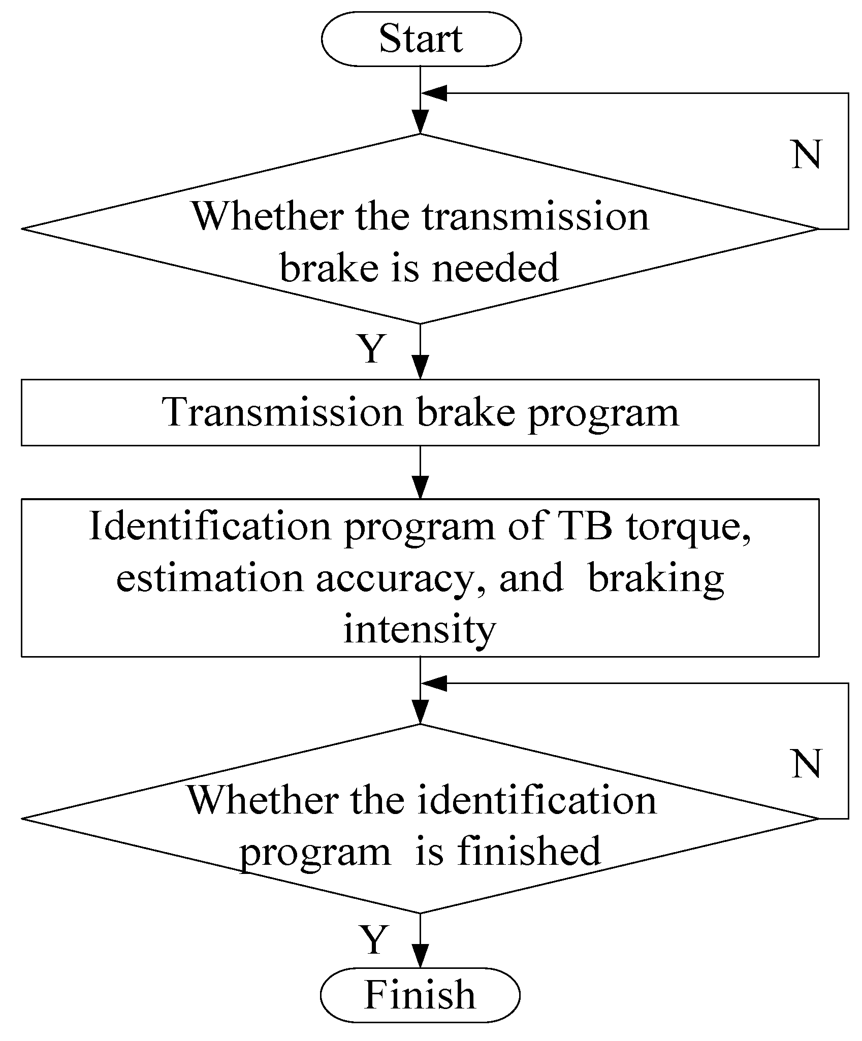
4.4. Identification Process of TB Characteristic Parameters
Parameter identification is completed in two situations. The first situation is when the estimation accuracy meets the requirements. The second situation is when the condition of the synchronous speed difference determined by the shifting schedule is met. The program of TB parameter identification is shown in Figure 7, including TB torque, estimation accuracy, and braking intensity.

Figure 7.
Flow of TB parameter identification.
5. Experimental Results
The test bench is shown in Figure 8. The rated speed of the power source (three-phase induction motor) was 980 rpm. The pressure of the AMT pneumatic system was about 7 bar. For the purpose of estimating the resistance torque of the AMT input shaft and TB characteristic parameters, the test data of the AMT input shaft’s speed were collected from the beginning time when the gear position was in neutral to the time when the speed decreased to 600 rpm, approximately.
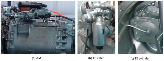
Figure 8.
Test bench.
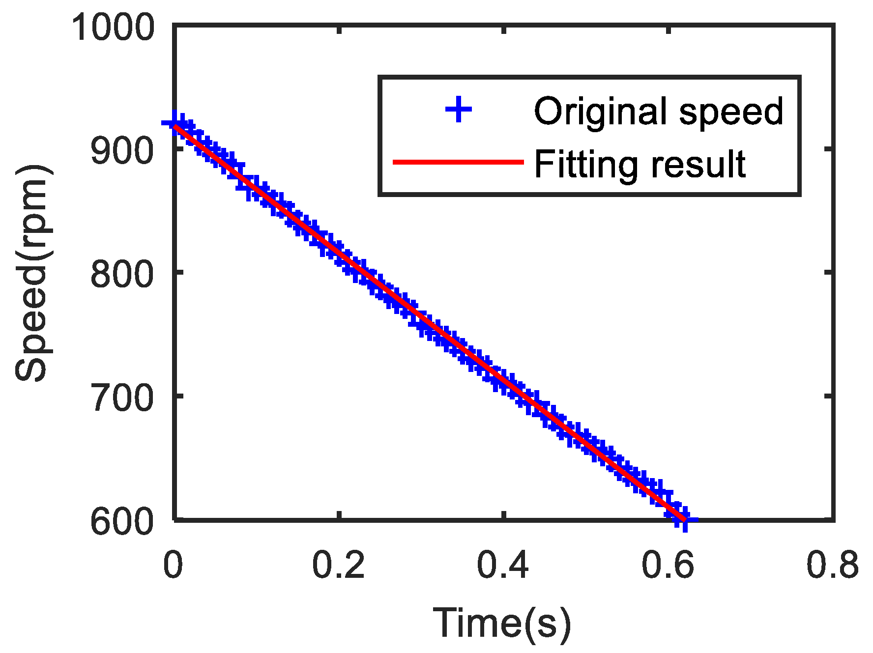
5.1. Estimation Results without TB Action
The inertia of the AMT input shaft was approximately 0.135 kg·m2. The AMT input shaft’s speed without TB action based on the least square fitting method is shown in Figure 9. The fitting error between the actual AMT input shaft’s speed without TB action and the fitting result is shown in Figure 10. As can be seen from Figure 10, the maximum fitting error and the minimum fitting error were 7.09 and 0.03 rpm. Consequently, the fitting curve can represent the original speed curve.
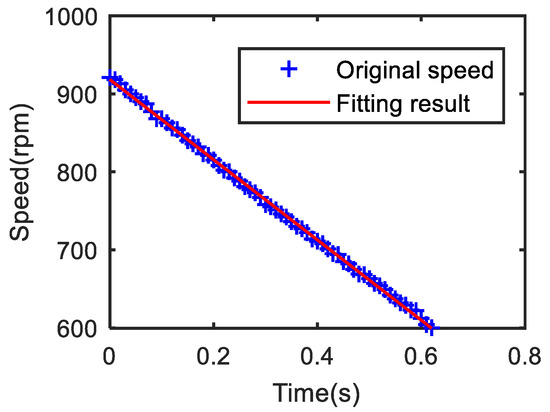
Figure 9.
Fitting result of AMT input shaft’s speed curve without TB action.
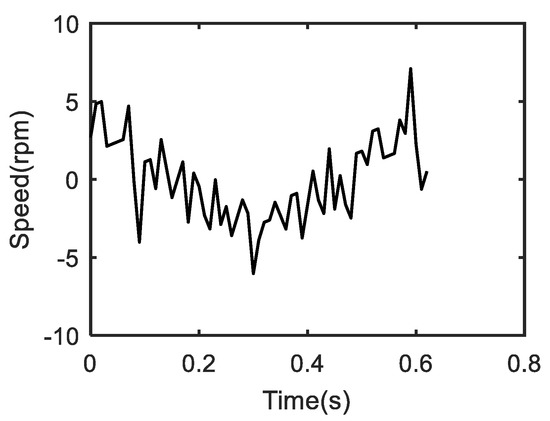
Figure 10.
Fitting error of AMT input shaft’s speed curve without TB action.
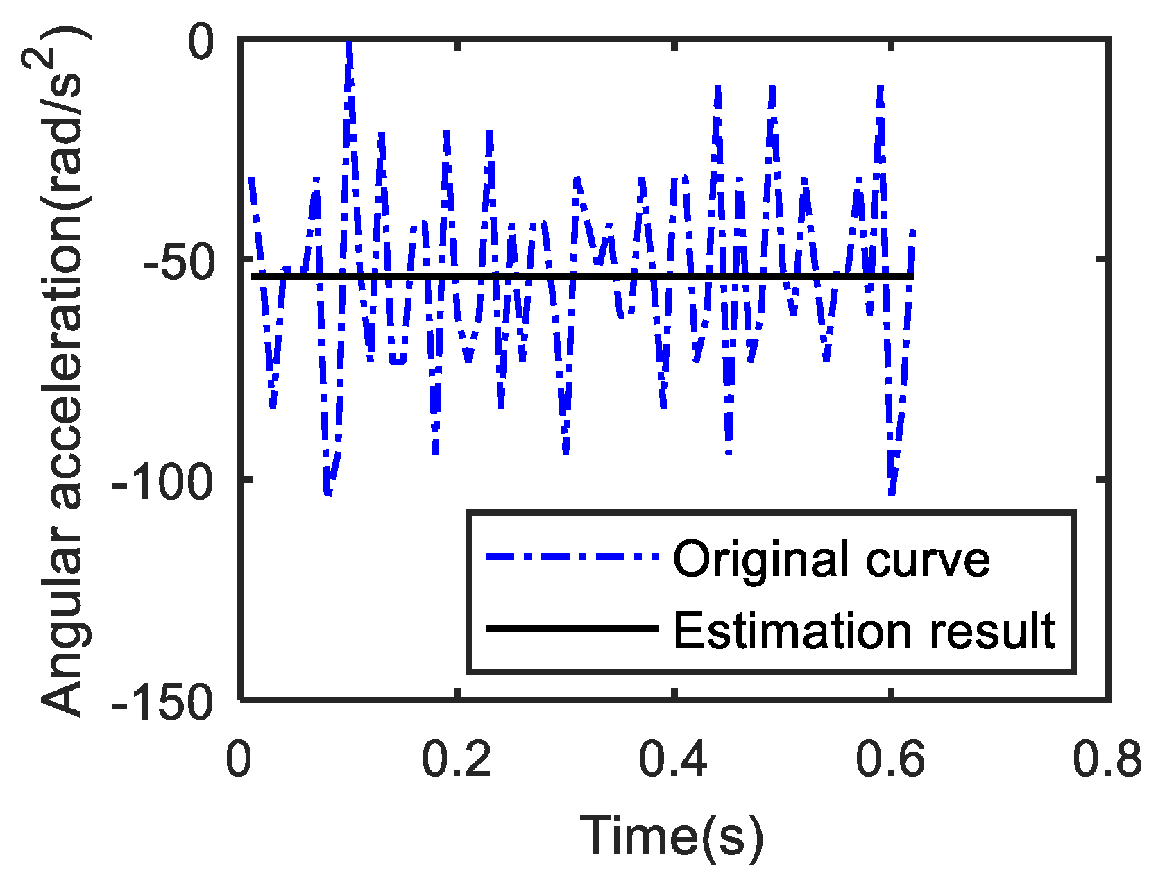
In accordance with Equation (12), the estimation result of the AMT input shaft’s angular acceleration was 53.85 rad/s2. To analyze the AMT input shaft’s angular acceleration fluctuations without TB action, the comparison between the AMT input shaft’s actual angular acceleration and estimation result without TB action is shown in Figure 11. The maximum and minimum of the angular acceleration errors between the original data and the estimation result were 53.85 and 1.49 rad/s2. For the AMT input shaft’s speed sensor, the AMT input shaft’s angular acceleration was calculated from the speed data and the sampling time. The smaller the sampling time, the bigger the angular acceleration error.
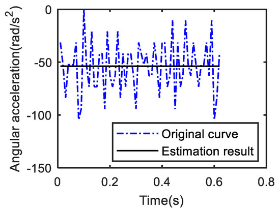
Figure 11.
Comparison between AMT input shaft’s angular acceleration and estimation without TB action.
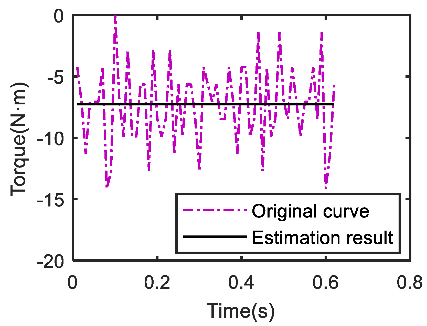
In accordance with Equation (12), the estimation result of the AMT input shaft’s equivalent resistance torque was −7.27 N·m. Based on the AMT input shaft’s actual angular acceleration, the AMT input shaft’s equivalent resistance torque can be calculated according to Equation (8). The comparison between the AMT input shaft’s equivalent resistance torque and estimation result is shown in Figure 12. The maximum and minimum of the torque errors between the original data and the estimation results were 7.27 and 0.20 N·m. The AMT input shaft’s equivalent resistance torque is calculated from the angular acceleration and its value is influenced by the AMT input shaft’s angular acceleration error. Thus, the higher the speed sensor, the more precise the estimation result.
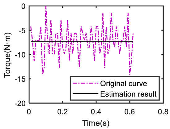
Figure 12.
Comparison between AMT input shaft’s equivalent resistance torque and estimation without TB action.
5.2. Estimation Results with TB Action
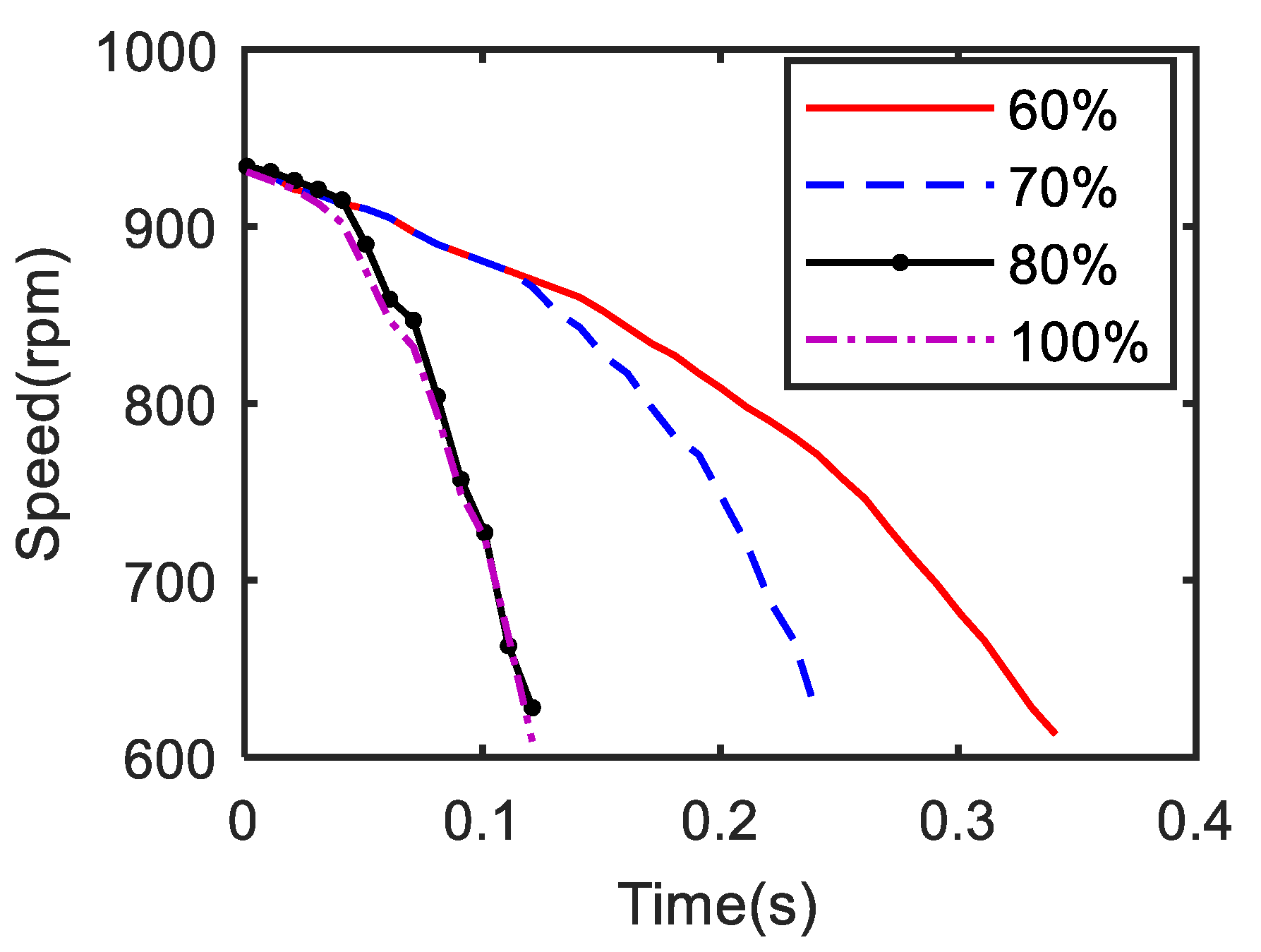
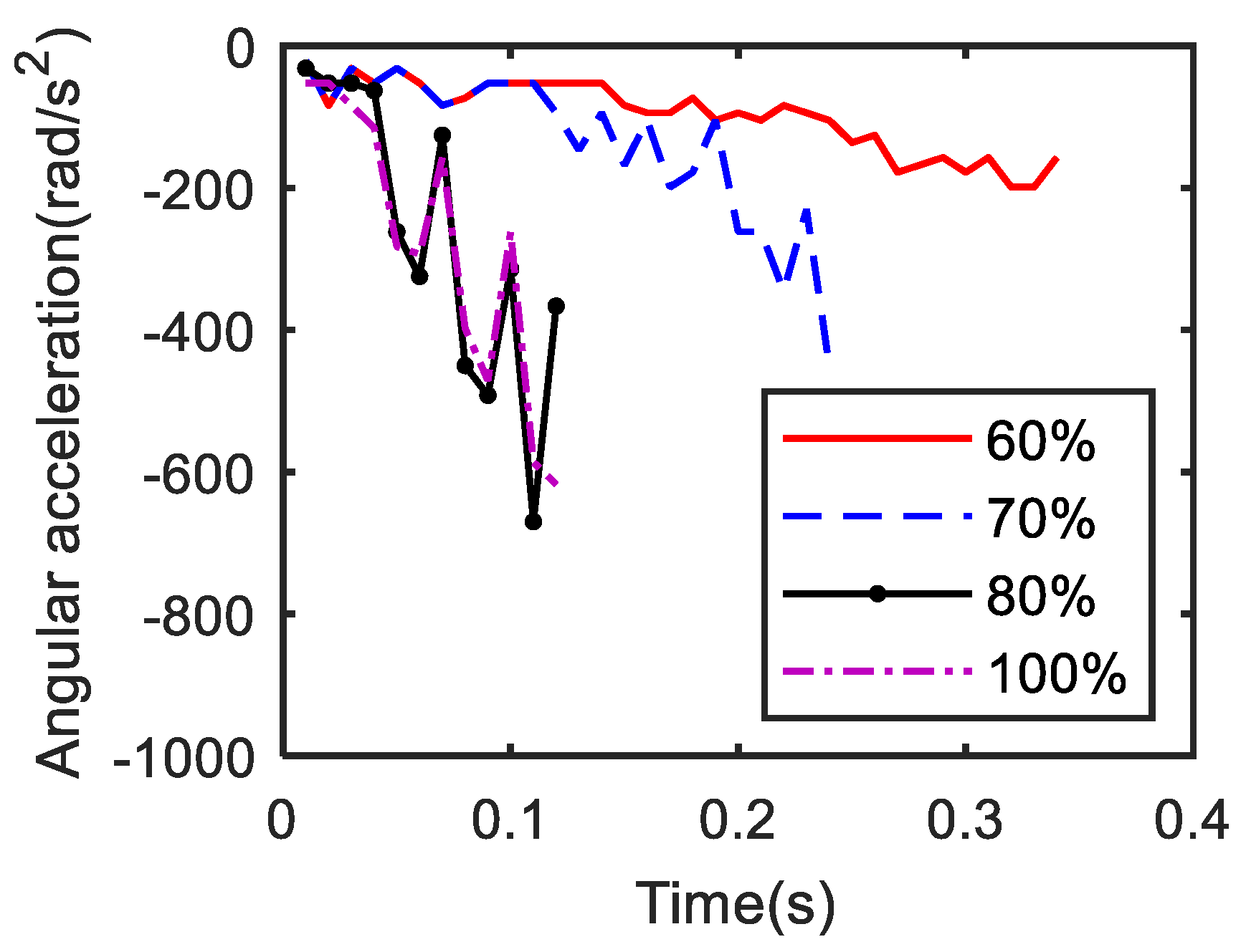
Figure 13 and Figure 14 show the AMT input shaft’s speed and angular acceleration under different duty cycles of 60%, 70%, 80%, and 100%, respectively. Figure 13 shows the whole deceleration processes are approximately 340, 230, 120, and 120 ms, respectively. It can be seen that the speed curves under the duty cycles of 80% and 100% are almost identical. It is indicated that the solenoid valve is fully open under the duty cycle of 80%. The four speed curves are consistent within 20 ms, showing that the lag time of braking action is approximately 20 ms under the duty cycle of 80%. Additionally, the lag times of braking action under the duty cycles of 60% and 70% are obviously longer than those under the duty cycles of 80% and 100%. The lag time of braking action greatly increases with the decreasing of the duty cycle of the TB solenoid valve. Thus, the completion time of the AMT input shaft’s deceleration process significantly decreases with the increasing of the duty cycle of the TB solenoid valve. Therefore, the TB action is directly related to the duty cycle of the TB solenoid valve.
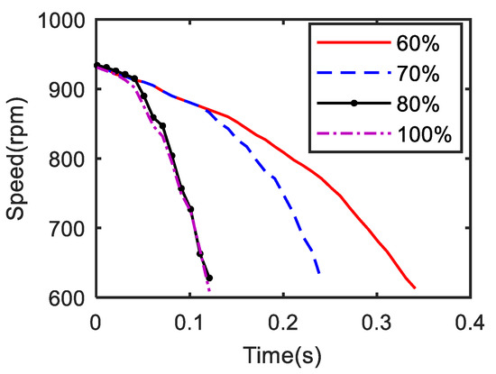
Figure 13.
AMT input shaft’s speed curves under different duty cycles of TB solenoid valve.
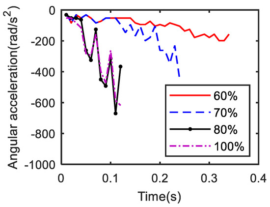
Figure 14.
AMT input shaft’s angular acceleration curves under different duty cycles of TB solenoid valve.
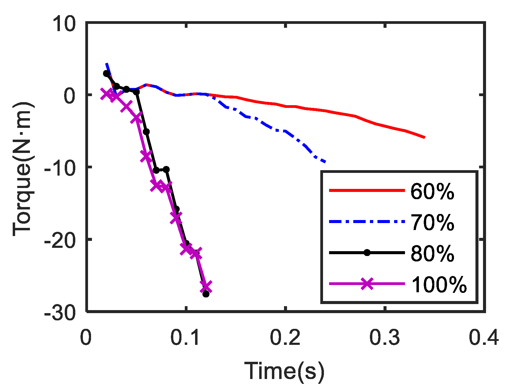
The braking characteristic parameters of TB action were studied according to the deceleration processes of AMT input shaft under the duty cycles of 60%, 70%, 80%, and 100%. Considering the effect of the measurement error, a Gaussian random white noise was added on the basis of the observer data. Its mean and variance were zero and 1, respectively. The weighting matrix is an identify matrix. In accordance with Equations (23)–(25), parameter estimations can be obtained under different duty cycles of the TB solenoid valve. The estimation results, including TB torque estimation, estimation accuracy, and braking intensity estimation are shown in Figure 15, Figure 16 and Figure 17, respectively.
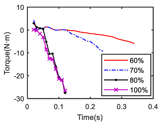
Figure 15.
TB torque estimation results under different duty cycles of TB solenoid valve.

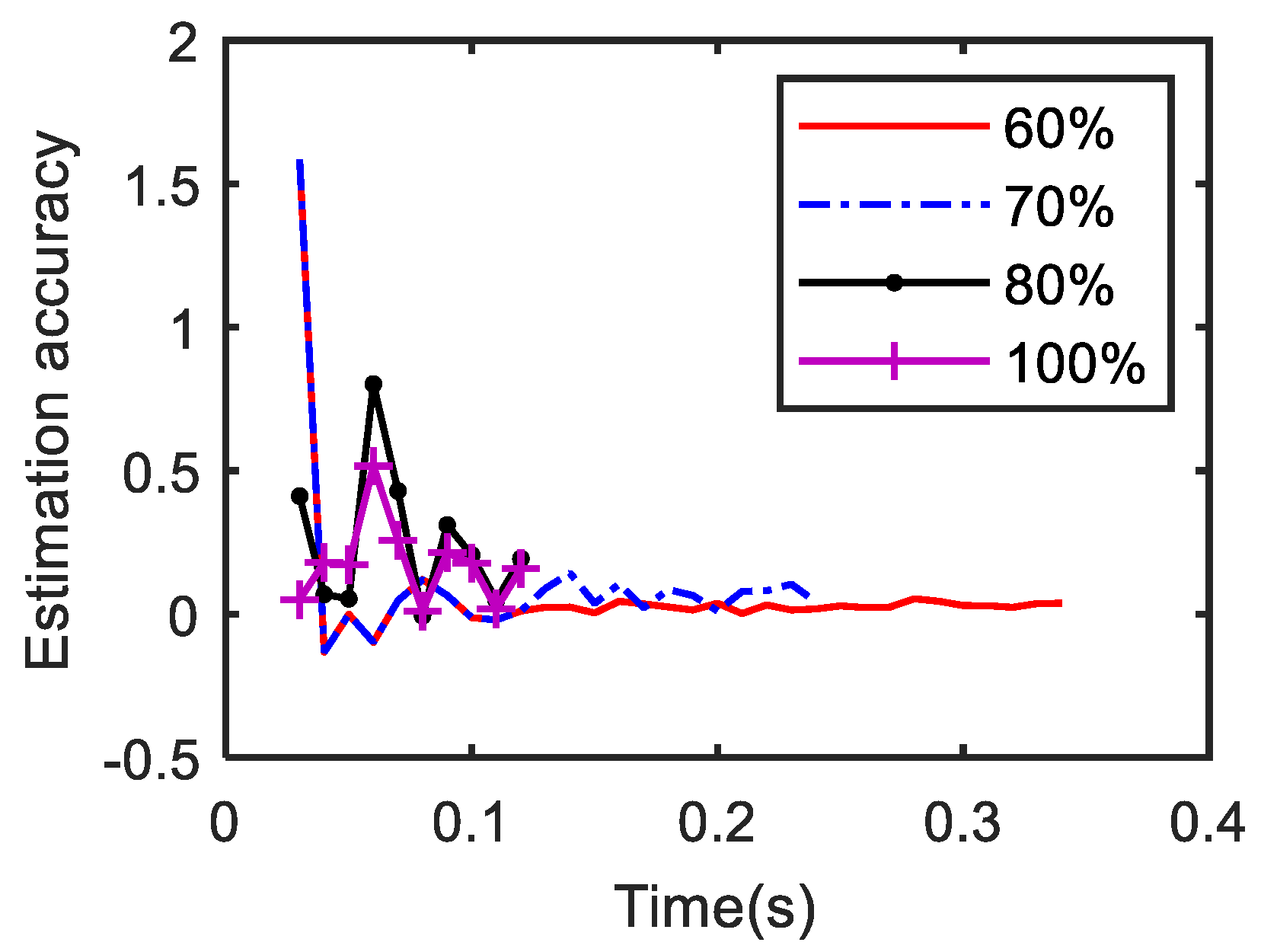
Figure 16.
Estimation accuracy results under different duty cycles of TB solenoid valve.

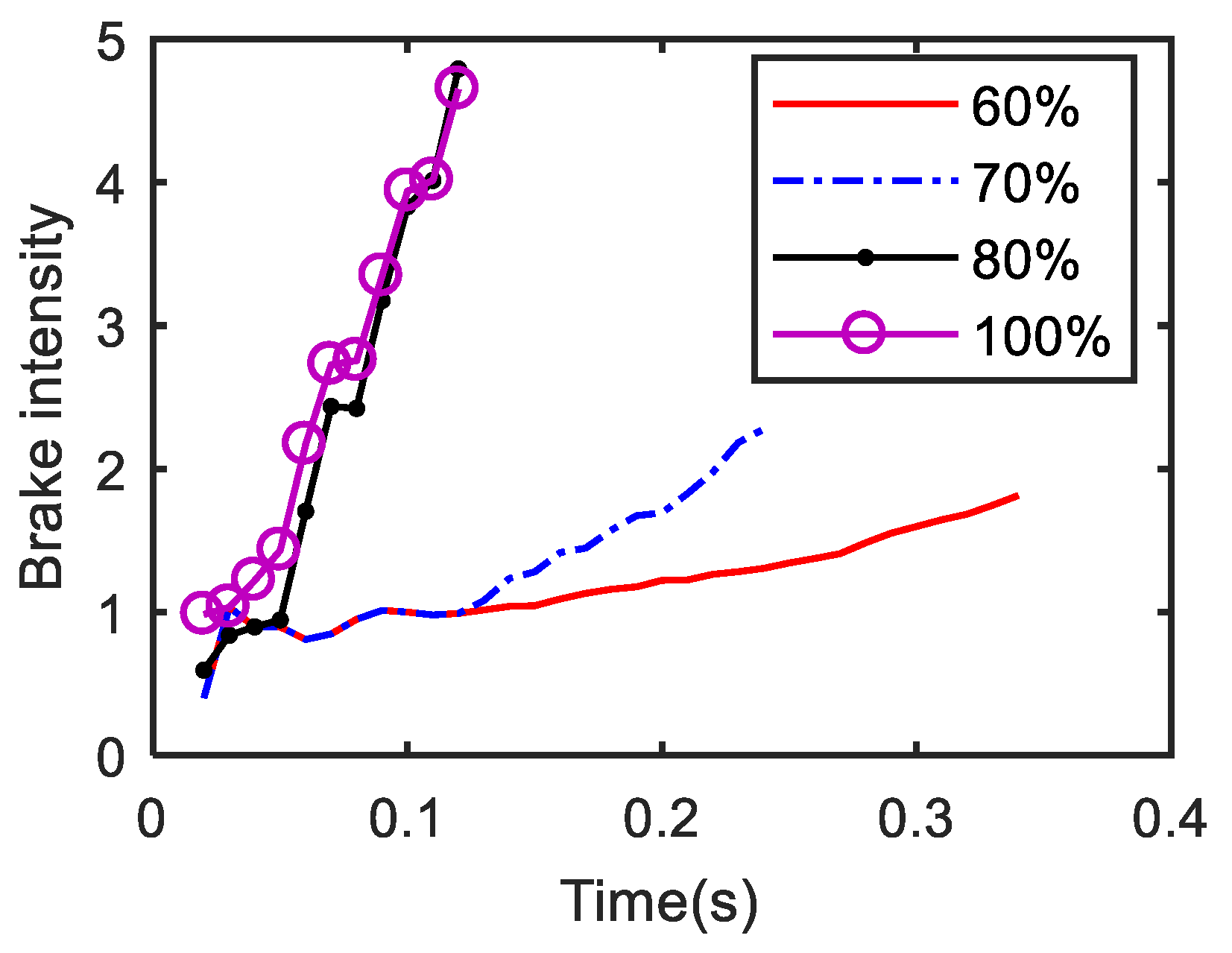
Figure 17.
Braking intensity estimation results under different duty cycles of TB solenoid valve.
Figure 15 shows the TB torque estimation results using the TB under the duty cycles of 60%, 70%, 80%, and 100%. The estimation values under different duty cycles are relatively small because of the lag times of the TB solenoid valve and TB cylinder. The estimation values of TB torque under the same duty cycle increase with the increasing of braking time. Obviously, the estimation value of TB torque increases with the increasing of the duty cycle of the TB solenoid valve. The two curves under the duty cycles of 80% and 100% are basically identical. The estimation values of TB torque under the duty cycle of 60% are clearly less than those under the duty cycle of 80%. The estimation values of TB torque at the moment of 700 rpm were −4.00, −7.10, −20.58, and −21.36 N·m, respectively under the duty cycles of 60%, 70%, 80%, and 100%. This means the estimation value of TB torque under the duty cycle of 100% was approximately five times as much as that under the duty cycle of 60%.
Figure 16 shows the estimation accuracy results using the TB under the duty cycles of 60%, 70%, 80%, and 100%. Obviously, the estimation accuracy changes significantly at the beginning because of TB action. With the increasing of measurement data, it becomes smaller. The estimation accuracies of TB torque at the moment of 700 rpm under the duty cycles of 60%, 70%, 80 and, 100% were 0.05%, 0.08%, 0.21%, and 0.18%, respectively. The values under the duty cycles of 60% and 70% are smaller because the braking times are longer, while those under the duty cycles of 80% and 100% are larger because the braking times are shorter.
Figure 17 shows the braking intensity results using the TB under the duty cycles of 60%, 70%, 80%, and 100%. The estimation value of braking intensity is approximately proportional to TB torque, where the curve trends are similar in Figure 15 and Figure 17. The estimation value of braking intensity increases with the increasing of the duty cycles of the TB solenoid valve. The estimation values of the braking intensity at the moment of 700 rpm under the duty cycles of 60%, 70%, 80, and 100% were 1.55, 1.97, 3.83 and 3.94, respectively. The braking intensity estimation under the duty cycle of 100% is more than two times as much as that under the duty cycle of 60%. In particular, the estimation value of braking intensity under the duty cycle 60% is extremely low, which can be used when the synchronous moment of the AMT input shaft, expressed by Equations (6) and (7), is approaching.
The synchronous moment of the AMT input shaft’s speed should be completed from 700 rpm to 800 rpm and the braking time should be completed within 200 ms to improve the upshifting quality and reduce the synchronous time. For the purpose of controlling the duty cycles of the TB solenoid valve and reducing the upshifting time, the comparisons of related parameter estimations are listed in Table 2 under different duty cycles and same AMT input shaft speeds.
Table 2.
TB braking estimations under different duty cycles.
The estimation value of braking intensity was only 1.22 when the AMT input shaft’s speed decreased to 800 rpm under the duty cycle of 60%, thereby failing to achieve the ideal shifting moment. Consequently, the value of the duty cycle should be larger at the beginning of controlling the TB.
5.3. Result Analysis
5.3.1. Linear Interpolation of Braking Intensity
To achieve synchronous shifting, the TB control should be finished within 200 ms to meet the synchronous speed difference condition. The value of the needed synchronous speed difference decreases with the increasing of the AMT output shaft’s resistance torque, which can be seen from Equation (7). In practice, the AMT input shaft’s speed is generally reduced to more than 700 rpm at the moment of synchronous shifting. So, the estimation results of TB characteristic parameters under the AMT input shaft’s speed of 800 rpm are regarded as the reference estimation values.
The braking intensity under the duty of any number can be obtained by linear interpolation method. The braking intensity under the duty cycle of any number from 60% to 80% can be achieved by Equation (26)
where is the value of the duty cycle, is the braking intensity under the duty cycle of , , , and are the braking intensity estimations under the duty cycles of 60%, 70% and 80%, respectively.
The total brake torque is the sum of the TB torque and the resistance torque of the AMT input shaft under the duty cycle of , it can be expressed as Equation (27), according to Equation (25)
5.3.2. Desired Speed Algorithm
Given the value of the synchronous speed difference according to Equation (7) and the realistic speed of the AMT output shaft at the upshifting moment, the AMT input shaft’s speed when the braking action is completed can be calculated as Equation (28), according to Equation (6)
where is the realistic speed value of the AMT input shaft when the TB action is completed.
Ignoring the damping, the desired speed curve using TB action can be calculated from Equation (29)
where is the AMT input shaft’s speed at the beginning of TB control, is the realistic braking time, is braking action time, and is the AMT input shaft’s speed at moment.
Given by the desired speed curve, the realistic AMT input shaft’s angular acceleration, expressed as , can be obtained. Then, the total brake torque and the braking intensity value can be predicted from Equations (13) and (25). Moreover, the realistic duty cycle of the solenoid valve can be predicted from Equation (27).
The response time of the TB actuator increases with the decreasing of the duty cycle of the TB solenoid valve from the above tests and estimations. To speed up the braking action and improve shifting quality, a larger value of the duty cycle for the solenoid valve should be used at the beginning of the TB controlling. The duty cycle of 80% is used first for 20 ms for starting the TB and then the TB solenoid valve is controlled by regulating the duty cycle using control methods.
6. Conclusions
The parameter estimation method of a countershaft brake for heavy-duty vehicles with AMT without synchronizer is studied in this paper. The AMT dynamic analysis is analyzed on the basis of the shifting model under the condition of clutch disengaging and putting the gear position in neutral. The TB analysis is examined on the basis of the TB model and the TB control flow is given. The estimation methods of the AMT input shaft’s running resistance torque without TB action and the TB characteristic parameters with TB action based on the RLSM are proposed. Using the experimental data of the AMT input shaft’s speed without TB action, the estimation of the AMT input shaft’s equivalent resistance torque is obtained. Using the experimental data of the AMT input shaft’s speed with TB action under different duty cycles of the TB solenoid valve, recursive estimations of the TB characteristic parameters, including the brake torque estimation, estimation accuracy and braking intensity estimation, are obtained. Linear interpolation algorithm of braking intensity from the duty cycle of 60% to that of 80% is given. The desired speed algorithm of the AMT input shaft using the TB are designed based on the experimental tests.
The running resistance torque of the AMT input shaft is affected by the working temperature, oil flow resistance, compressed air pressure, and mechanical friction resistance. As a result, some errors between the estimation results and the actual values for the AMT input shaft’s equivalent resistance torque and TB torque will be presented in the use process of AMT. Some measurement errors of the AMT input shaft’s speed may also exist according to the measuring accuracy problem. The estimation results of the TB characteristic parameters are affected by these physical factors, but these data provide some major characteristics of TB action. The experimental results show that the estimation methods are effective and provide an experimental basis for further studying the shift schedule for heavy-duty vehicles with AMT without synchronizer.
Author Contributions
Conceptualization, Y.L.; methodology, Y.L.; software, Y.L.; validation, L.L.; formal analysis, Y.L.; investigation, L.L.; resources, Y.L.; data curation, Y.L.; writing—original draft preparation, Y.L.; writing—review and editing, Y.L.; visualization, L.L.; supervision, Y.L.; project administration, Y.L.; funding acquisition, L.L. Both authors have read and agreed to the published version of the manuscript.
Funding
This research was funded by Key R & D Project of Shandong Province, China, grant number 2020CXGC11003.
Institutional Review Board Statement
Not applicable.
Informed Consent Statement
Not applicable.
Data Availability Statement
Not applicable.
Acknowledgments
This work was supported by Key R & D Project of Shandong Province, China (Grant No. 2020CXGC011003).
Conflicts of Interest
The authors declare no conflict of interest.
References
- Mo, W.; Wu, J.; Walker, P.D.; Zhang, N. Shift characteristics of a bilateral Harpoon-shift synchronizer for electric vehicles equipped with clutchless AMTs. Mech. Syst. Signal Process. 2021, 148, 107166. [Google Scholar] [CrossRef]
- Mo, W.; Walker, P.D.; Tian, Y.; Zhang, N. Dynamic analysis of unilateral harpoon-shift synchronizer for electric vehicles. Mech. Mach. Theory 2021, 157. [Google Scholar] [CrossRef]
- Chen, B.; Guo, J.; Yan, M.F.; Wang, F.; Liu, F. Study on a Ni-P-nano TiN composite coating for significantly improving the service life of copper alloy synchronizer rings. Appl. Surf. Sci. 2020, 504. [Google Scholar] [CrossRef]
- Barathiraja, K.; Devaradjane, G.; Jibin, P.; Rakesh, S.; Gajanan, J. Analysis of automotive transmission gearbox synchronizer wear due to torsional vibration and the parameters influencing wear reduction. Eng. Fail. Anal. 2019, 105, 427–443. [Google Scholar] [CrossRef]
- Barathiraja, K.; Devaradjane, G.; Bhattacharya, A.; Sivakumar, V.; Yadav, V. Automotive Transmission Gearbox Synchronizer Sintered Hub Design. Eng. Fail. Anal. 2020, 107. [Google Scholar] [CrossRef]
- Eckert, J.J.; Santiciolli, F.M.; Yamashita, R.Y.; Correa, F.C.; Silva, L.C.A.; Dedini, F.G. Fuzzy gear shifting control optimization to improve vehicle performance, fuel consumption and engine emissions. IET Control Theory Appl. 2019, 13, 2658–2669. [Google Scholar] [CrossRef]
- Lin, S.; Li, B. Shift force optimization and trajectory tracking control for a novel gearshift system equipped with electromagnetic linear actuators. IEEE-ASME Trans. Mechatron. 2019, 24, 1640–1650. [Google Scholar] [CrossRef]
- Myklebust, A.; Eriksson, L. Modeling, observability, and estimation of thermal effects and aging on transmitted torque in a heavy duty truck with a dry clutch. IEEE-ASME Trans. Mechatron. 2015, 20, 61–72. [Google Scholar] [CrossRef]
- Gao, B.; Lu, X.; Chen, H.; Lu, X.; Li, J. Dynamics and control of gear upshift in automated manual transmissions. Int. J. Veh. Des. 2013, 63, 61–83. [Google Scholar] [CrossRef]
- Gao, B.; Chen, H.; Ma, Y.; Sanada, K. Design of nonlinear shaft torque observer for trucks with Automated Manual Transmission. Mechatronics 2011, 21, 1034–1042. [Google Scholar] [CrossRef]
- Zhang, H.; Zhao, X.; Sun, J. Optimal clutch pressure control in shifting process of automatic transmission for heavy-duty mining trucks. Math. Probl. Eng. 2020, 2020. [Google Scholar] [CrossRef]
- Meng, F.; Zhang, H.; Cao, D.; Chen, H. System modeling and pressure control of a clutch actuator for heavy-duty automatic transmission systems. IEEE Trans. Veh. Technol. 2016, 65, 4865–4874. [Google Scholar] [CrossRef]
- Zhang, H.; Zhao, X.; Yang, J.; Zhang, W. Optimizing automatic transmission double-transition shift process based on multi-objective genetic algorithm. Appl. Sci. 2020, 10, 217794. [Google Scholar] [CrossRef]
- Nakazawa, T.; Hattori, H.; Tarutani, I.; Yasuhara, S.; Inoue, T. Influence of pin profile curve on continuously variable transmission (CVT) chain noise and vibration. Mech. Mach. Theory 2020, 154. [Google Scholar] [CrossRef]
- Zhao, H.; Liu, C.; Song, Z.; Liu, S. A Consequent-pole PM magnetic-geared double-rotor machine with flux-weakening ability for hybrid electric vehicle application. IEEE Trans. Magn. 2019, 55. [Google Scholar] [CrossRef]
- Onumata, Y.; Zhao, H.; Wang, C.; Morina, A.; Neville, A. Interactive Effect between Organic Friction Modifiers and Additives on Friction at Metal Pushing V-Belt CVT Components. Tribol. Trans. 2018, 61, 474–481. [Google Scholar] [CrossRef]
- Zhao, Z.; Lei, D.; Chen, J.; Li, H. Optimal control of mode transition for four-wheel-drive hybrid electric vehicle with dry dual-clutch transmission. Mech. Syst. Signal Process. 2018, 105, 68–89. [Google Scholar] [CrossRef]
- Zhao, Z.; Li, X.; He, L.; Wu, C.; Hedrick, J.K. Estimation of Torques Transmitted by Twin-Clutch of Dry Dual-Clutch Transmission during Vehicle’s Launching Process. IEEE Trans. Veh. Technol. 2017, 66, 4727–4741. [Google Scholar] [CrossRef]
- Schoeftner, J.; Ebner, W. Simulation model of an electrohydraulic-actuated double-clutch transmission vehicle: Modelling and system design. Veh. Syst. Dyn. 2017, 55, 1865–1883. [Google Scholar] [CrossRef]
- Bóka, G.; Lovas, L.; Márialigeti, J.; Trencséni, B. Engagement capability of face-dog clutches on heavy duty automated mechanical transmissions with transmission brake, Proceedings of the Institution of Mechanical Engineers. Part D J. Automob. Eng. 2010, 224, 1125–1139. [Google Scholar] [CrossRef]
- Li, W.; Gong, G.; Liu, J.; Zhang, Y.; Yang, H. Simulation of electro-hydraulic system for train brake based on pressure control of high frequency solenoid valve. J. Cent. South Univ. (Sci. Technol.) 2020, 51, 340–348. [Google Scholar] [CrossRef]
- Zhao, J.; Zhou, Y.; Shi, Y.; Wang, Z.; Ma, X.; Song, E. Experimental research of dynamic response of high speed solenoid valve for common rail injecto. Harbin Gongcheng Daxue Xuebao/J. Harbin Eng. Univ. 2018, 39, 74–79. [Google Scholar] [CrossRef]
- Gao, Q.; Zhu, Y.; Luo, Z.; Bruno, N. Investigation on adaptive pulse width modulation control for high speed on/off valve. J. Mech. Sci. Technol. 2020, 34, 1711–1722. [Google Scholar] [CrossRef]


Publisher’s Note: MDPI stays neutral with regard to jurisdictional claims in published maps and institutional affiliations. |
© 2021 by the authors. Licensee MDPI, Basel, Switzerland. This article is an open access article distributed under the terms and conditions of the Creative Commons Attribution (CC BY) license (https://creativecommons.org/licenses/by/4.0/).