Article

The Bi-Level Optimal Configuration Model of the CCHP System Based on the Improved FCM Clustering Algorithm

1
State Key Laboratory of Eco-Hydraulics in Northwest Arid Region, Xi’an University of Technology, Xi’an 710048, China
2
School of Electrical Engineering, Xi’an University of Technology, Xi’an 710048, China
3
Xi’an Electric Power Supply Company, State Grid Shaanxi Electric Power Company, Xi’an 710032, China
4
Gansu Electric Power Research Institute, State Grid Gansu Electric Power Company, Lanzhou 730050, China
*
Author to whom correspondence should be addressed.
Processes 2021, 9(6), 907; https://doi.org/10.3390/pr9060907
Submission received: 8 April 2021 / Revised: 13 May 2021 / Accepted: 18 May 2021 / Published: 21 May 2021

Abstract

:
To improve the comprehensive benefits of the CCHP system, this paper proposes a bi-level optimal configuration model of the CCHP system based on the improved FCM clustering algorithm. Firstly, based on the traditional FCM clustering algorithm, the entropy method is used to introduce the PFS index and the Vp index in a weighted form to achieve a comprehensive evaluation of the clustering effect. The effectiveness of the improved FCM algorithm is verified by analyzing the clustering process of the load and meteorological data using the improved FCM algorithm. Then the best cluster number and fuzzy coefficient is found using the traversal method. Secondly, a bi-level configuration optimization model is constructed. The outer layer is the configuration optimization layer, and the inner layer is the operation optimization layer. The model is solved by combining the NSGA-II and PSO algorithms. Finally, a bi-level optimal configuration model is constructed for actual cases, and the clustering results of the improved FCM algorithm are brought into the model. The example calculation analyses show that, compared with existing methods, the proposed method significantly reduces the operating cost and carbon dioxide emissions of the CCHP microgrid.

1. Introduction

The combined cooling, heating, and power (CCHP) system is a multi-energy integrated supply system with cogeneration equipment as its core, including multiple distributed units, such as power generation and energy storage, and multiple energy forms, including cooling, heating, and electricity [1]. CCHP is established based on energy cascade utilization, using primary energy to drive generators to generate electricity and then recover waste heat through various types of waste-heat utilization equipment, which improves energy utilization, has lower energy costs, a higher safety, and better environmental protection [2]. In addition, in view of the uncertainty and intermittency of clean renewable energy, such as wind power and photovoltaics, CCHP could be combined with wind power and photovoltaics to provide effective support for the development and utilization of distributed energy [3].
The economical and efficient operation of CCHP needs to solve the problem of dynamic energy balance between system supply and user demand. The user-side demand changes in real-time, so when the configuration is unreasonable, not only can the energy-saving effect not be achieved, but it will increase the system’s energy consumption [4]. Therefore, according to the load changes and the actual needs of users, realizing the core equipment parameter design and system optimization configuration, reasonably planning on equipment investment in the early stages, and accurately matching the energy supply and demand relationship as well as the coupling relationship of energy flow are essential prerequisites for the efficient operation of the system [5].
Domestic and foreign research on the optimization configuration of CCHP is mainly reflected in the following three aspects: (1) Different optimization goals. The general optimization goals are energy-saving, economy, and environmental protection. Presently, some scholars also list other optimization goals into the scope of consideration; specifically, investment and operating costs [4,5,6], carbon dioxide emissions [4,5,6], energy utilization efficiency [4,5,6], load power supply reliability [7], clean energy consumption rate [8], etc. (2) Different optimization objects. Due to the different use environments and purposes of CCHP, the input system’s source-load characteristics and configuration focus are also different [9]. For example, there is an optimization configuration problem for buildings, such as hospitals, hotels, office buildings, and residential buildings [10], and there is also an optimization configuration problem of the CCHP microgrid for an industrial park or an island [11]. (3) Existing research mainly adopt two methods to deal with the operation mode while conducting configuration optimization: a given set of fixed operation modes and the construction of a bi-level model for operation optimization [4,12]. The former cannot give full play to the complementary cooperation capabilities between various devices (especially energy storage devices), and cannot achieve optimal operation, which, in turn, affects the configuration optimization of the system. The latter has the problem of a large amount of calculations [13].
The optimization of the CCHP configuration needs to consider many factors. In the optimization model, long-term relevant data are generally needed for evaluation; usually a large amount of weather, load, and other data. However, although a large amount of data can ensure optimization result accuracy as much as possible, it greatly increases the amount of calculations. To overcome this problem, scholars have proposed using the clustering algorithm to reduce scenes; replacing a large number of scene features with a small number of scenes [14].
Fuzzy C-means (FCM) is a widely used clustering method. Unlike hard clustering, in which each sample object can and can only be classified into one class, FCM introduces the concept of membership degrees. When applying FCM clustering, each sample can belong to two or more classes with a certain membership degree, which is very suitable for the clustering requirements of meteorological and load data [15]. However, FCM itself has many shortcomings; for example, it is difficult to determine the optimal cluster number and the choice of the fuzzy degree coefficients will significantly affect clustering results [16]. The fuzzy degree coefficients are an important parameter in FCM, and their values determine the clustering result’s fuzzy degree. In most of the existing research and applications of FCM, the value of the fuzzy degree is usually the default value, but different fuzzy degree values have a significant impact on clustering results [17]. In addition to this, the value of a cluster number also has a very large impact on subsequent calculations. A cluster number that is too large is not conducive to solving calculations, and, if too small, a cluster number will not be comprehensive. The cluster validity index is often used to evaluate the quality of different cluster divisions [18]. Therefore, this paper proposes an improved FCM algorithm suitable for load and weather scene reduction, starting from the cluster validity test, which can automatically find the optimal cluster number and fuzzy degree coefficients according to data distributions.
The existing literature has proposed many improved FCM algorithms for different research problems. The authors in [19] proposed an improved Canopy–FCM algorithm based on the max–min principle in order to solve the problem of the FCM algorithm being sensitive to the initial clustering center. Use of the parallel computing framework of MapReduce helped to realize the improved Canopy-FCM algorithm. The experimental results showed that the improved Canopy–FCM algorithm based on MapReduce had better clustering quality and running speed than Canopy–FCM and FCM. The authors in [20] proposed generalized FCM and hierarchical FCM to solve the problem of FCM’s insufficient robustness to image noise and the sensitivity of Euclidean distance in FCM to outliers. The experimental results proved the robustness and effectiveness of the proposed algorithm. In [21], an improved FCM clustering algorithm was proposed for the problems of long iteration times, long convergence times, and the low accuracy of the FCM clustering algorithm. In addition, the improved FCM was used for the clustering of web log data. In [22], the concept of similarity was proposed and replaced the traditional similarity matrix with a similarity matrix, which improved FCM. However, the improvements to FCM in the abovementioned literature only focuses on the influence of the number of clusters on the clustering result, and do not consider the influence of the fuzzy coefficient on the clustering results. Related research shows that the fuzzy coefficient has a significant impact on clustering results, and the default fuzzy coefficient is not necessarily the best.
The existing literature has proposed many methods to determine the optimal number of clusters. In [23], in order to solve the problem of the large amount of calculations in using the validity index to determine the number of clusters, a method of using the R package “kpeaks” to quickly determine the optimal number of clusters before the start of clustering was proposed. In [24], a new adaptive fuzzy C-means clustering algorithm (A-FCM) based on the idea of hierarchical clustering was proposed in view of the shortcomings of traditional fuzzy clustering algorithms, which cannot automatically determine the number of clusters. Numerical experiments showed that this method had better results. A novel fuzzy clustering validity evaluation index has been proposed in the literature [25], and the simulation experimental results show that the proposed validity function can effectively partition a dataset. However, the abovementioned literature did not consider the influence of fuzzy coefficients on the clustering results when searching for the optimal number of clusters.
According to different components, a cluster validity index can be divided into the cluster validity index considering the dataset’s geometric structure information and the cluster validity index considering the membership degree [26]. Among these, the dataset’s geometric structure information refers to the information extracted from data partition features, such as compactness, separation, connectivity, and overlap degree. At present, the commonly used cluster validity indices that considers the geometric structure of the dataset mainly include: Dunn, CH, G, CI, DB, Sil, I, CS, SF, COP, SV, OS, etc. [26,27]. The abovementioned indicators only consider the geometric structure information in the clustering results. The scope of the application of most indicators is not clear. They perform well on general datasets, but, on some complex datasets, such as those with more noise points or a large overlap between classes, it is not always possible to determine optimal clustering results nor the optimal cluster number. In addition, although these indicators that only consider data partition information can also be used to evaluate the effectiveness of fuzzy clustering, they do not perform well in fuzzy clustering because they do not consider the membership degree and fuzzy degree in fuzzy clustering.
The fuzzy clustering validity indices that consider membership degree mainly include: the partition coefficient (PC) and partition entropy (PE), normalized partition coefficient (NPC) and normalized partition entropy (NPE), KYI, Vp, OS, etc. [28,29,30,31,32]. The indicators above only consider the membership degree information in the fuzzy division, and they usually experience the following three problems: (1) with a change in cluster number, the trend is monotonous; (2) they are sensitive to the value of the fuzzy coefficient; and (3) because the geometric structure information of clustering is not used, these indicators lack a direct connection to the dataset’s geometric structure. Although most of the validity indicators that consider membership degree are relatively simple and have a small number of calculations, they are not ideal in accurately evaluating the cluster’s quality and correctly identifying the cluster number.
Based on the above analysis, this paper makes the following contributions to the studied problems:
(1)
It improves the FCM clustering algorithm and introduces the PFS index to evaluate a dataset’s geometric structure validity and the Vp index is used to evaluate the membership degree validity. It combines the two indexes using the entropy method to comprehensively evaluate the clustering effectiveness. Afterward, the traversal method automatically finds the optimal cluster number and fuzzy degree coefficients according to the data distribution.
(2)
It constructs a bi-level CCHP optimization configuration model. The outer layer is the configuration optimization layer, and the inner layer is the operation optimization layer. Additionally, it brings the clustering results of the improved FCM algorithm into the model. For actual cases, the feasibility and effectiveness of the proposed method are verified through comparative analyses.

2. Improved FCM Clustering Algorithm

2.1. FCM Clustering Algorithm

FCM is a typical and widely used fuzzy clustering method. The algorithm is based on a given cluster number and cluster centers, and constantly updates the membership degree and cluster centers. The objective function is minimized until the cluster center no longer changes or the difference between the objective function values of the two iterations is within the allowable range [33]. The objective function of clustering is:
{ J c ( U , V ) = C i C x j C i μ i j m d ( x j , v i ) v i = 1 n i x j C i x j ,
where V is the cluster center matrix, V = { v 1 , v 1 , , v c } . v i is the cluster center of the i-th category C i . n i is the number of samples in the i-th category C i . d ( x j , v i ) is the Euler distance from sample x j to center v i of class C i . m is the fuzzy coefficient.
The updated formulas of membership degree μ i j and cluster center v i are:
{ μ i j = 1 r = 1 c [ d ( x j , v i ) d ( x j , v r ) ] 2 m 1 v i = j = 1 n μ i j m x j / j = 1 n μ i j m ,
FCM has the following shortcomings. First, the cluster number of the FCM needs to be given in advance, and different initialization condition settings will result in different clustering results. Second, the concept of the fuzzy degree is introduced in FCM, and different values of fuzzy degree have a greater impact on the performance of the algorithm. Therefore, it is necessary to determine the optimal number of clusters and fuzzy coefficients to avoid affecting the rationality and effectiveness of the clustering results.

2.2. Fuzzy Clustering Validity Index

According to the different components of the cluster validity index, it can be divided into a cluster validity index, considering the geometric structure information of the data set, and cluster validity index considering the degree of membership. The former can be used, not only for hard clustering, but also for validity tests of fuzzy clustering. The latter can only be used to evaluate the effectiveness of fuzzy clustering [26]. According to the analysis in the introduction, these two types of clustering effectiveness indicators have their own advantages and disadvantages, and they cannot be used on their own to comprehensively evaluate clustering results.
Therefore, in order to comprehensively evaluate the pros and cons of the FCM clustering results, this paper introduces PFS, considering the effectiveness of the geometric structure information clustering of the dataset and Vp considering the effectiveness of the membership degree clustering on the basis of the original algorithm. Additionally, the entropy method is used to combine the two in a weighted form to form a comprehensive clustering evaluation index.

2.2.1. PFS

Pseudo F-statistics (PFS) is a statistic from the field of analysis of variance (ANOVA). For a sample of P (P ≥ 1) dimensional variables, “pseudo-F statistical ratio” is defined as follows [34]:
P F S = tr ( S B P ) ( m - c ) tr ( S W P ) ( c - 1 ) ,
where tr ( S B P ) and tr ( S W P ) are the traces of matrix S B P and S W P . m is the number of samples. c is the number of clusters. S B P and S W P are the inter-class and intra-class scatter matrices of P-dimensional variable samples, respectively, and their expressions are as follows:
{ S B P = i = 1 c j = 1 m μ i j v i v i T S W P = i = 1 c j = 1 m μ i j ( x j - v i ) ( x j - v i ) T ,
where x j is the j-th sample vector. v i is the cluster center of the i-th class. The expression of μ i j is as follows:
μ i j = { 0 x j C i 1 x j C i ,
In [34], it was pointed out that, as the c increases, the PFS value first rises and then decreases continuously. That is, the PFS may reach a maximum value at a certain c value, and that value is the optimal cluster number. Finding the optimal cluster number (c) is equivalent to finding the maximum PFS value.
The PFS index [34] and the CH+ index [35] have exactly the same structure. In [36], if was concluded that the performance of the CH+ index was the best in a comparative study of 30 clustering effectiveness indexes [34]. The authors of [33] performed a clustering result evaluation test for many clustering evaluation indicators, and the results proved that CH+ has a good performance. In [37], it was pointed out that the PFS index is closely related to data distribution.

2.2.2. Vp

The authors of [32] proposed the definition of the Vp index as:
{ V p ( U ) = 1 n k = 1 n max i ( μ i k ) 1 K i = 1 p 1 j = i + 1 p [ 1 n k = 1 n min ( μ i k , μ j k ) ] K = p ( p 1 ) 2 ,
It can be seen that cluster validity measure Vp, is composed of two items. The first item reflects the compactness within a cluster. The closer kth sample x k is to a fuzzy cluster center, the closer the maximum membership degrees ( max ( μ i k ) ) is to the value of 1. Hence, fuzzy set max ( μ i k ) is considered as a good indicator of the clustering quality for each pattern ( x k ). On the other hand, the second item indicates the separation among clusters. In fact, if x k is close to the fuzzy cluster center of v i , k = 1 n min ( μ i k , μ j k ) comes close to 0, and consequently fuzzy sets U i and U j are clearly separated. If k = 1 n min ( μ i k , μ j k ) is close to 1 / p , x k belongs to all clusters that have equal membership degree and the fuzziest separation is unclear. The validity (Vp) criterion combines fuzzy compactness and separation.
The authors of [32] pointed out that, although the existing literature has proposed many clustering effectiveness indicators that consider the degree of membership, these indicators are not applicable when fuzzy parameter m changes in a relatively large range. When m changes in a relatively large range, the Vp index still has the ability to effectively evaluate the results of FCM clustering. According to experimental results, the proposed validity index (Vp) works very well in the range of m [ 1.5 , 5 ] , which is quite usual in practice (m = 2 is, thus far, the most common choice) [32].

2.3. The Entropy Method

The entropy method is an objective method of determining weight, which borrows the concept of entropy from information theory. The information entropy in the information system is a measure of the disorder degree of information. The greater the information entropy, the higher the disorder degree of the information and the smaller the information’s utility value. Conversely, the smaller the information entropy, the smaller the disorder degree of the information, and the greater the utility value of the information. For example, in terms of a certain attribute, when all schemes have the same result, this attribute plays a small role in decision-making. When all selected schemes have no difference under this attribute, this attribute can even be omitted.
For the obtained matrix, X = ( x i j ) m × n , the specific steps of the entropy method are as follows [38]. m is the number of alternatives and n is the target number.
(1)
Calculate the standardized matrix R = ( r i j ) m × n ,
r i j = max { x 1 j , x 2 j , , x m j } x i j max { x 1 j , x 2 j , , x m j } min { x 1 j , x 2 j , , x m j } , i = 1 , 2 , m ; j = 1 , 2 , n ,
(2)
Calculate the information entropy e j of each target,
{ e j = k i = 1 m r i j ln r i j k = 1 / ln ( m ) ,
(3)
Calculate the weight w j of each target,
{ w j = h j j = 1 n h j h j = 1 e j ,

2.4. The Calculation Process of Improved FCM Clustering Algorithm

On the basis of the traditional FCM clustering algorithm, this paper introduces the PFS index to evaluate the validity of the geometric structure of a dataset, and the Vp index is used to evaluate the validity of the membership degree. The entropy method is used to weight the two indicators to comprehensively evaluate the effect of clustering. Then, the best cluster number (c) and fuzzy coefficient (m) are determined using the traversal method. Supposing that the total amount of input data is n, to ensure the calculation speed, the clustering result is generally not greater than n . In addition, the authors of [39] pointed out that the best value range of m is [1,5]. The flow chart of the improved FCM clustering algorithm is shown in Figure 1.
(1)
Suppose the amount of input data is n. Set the fuzzy coefficient, m = 1.1, and the number of clusters, c = 2.
(2)
Use the FCM algorithm to cluster the input dataset to obtain the clustering result, S.
(3)
Calculate the PFS index and Vp index of the clustering result, S, and save them to vectors y1 and y2, respectively.
(4)
The number of clusters, c, increases by 1, repeat steps (2)–(3) until the number of clusters is greater than n . Obtain the PFS index vector y1 and Vp index vector y2 of different cluster numbers under the same fuzzy coefficient.
(5)
According to the entropy weight method described in Section 2.3., use y1 and y2 to calculate the weights, w1 and w2, of the two indicators.
(6)
Calculate the comprehensive evaluation index vector, y3 = w1*y1 + w2*y2, corresponding to the fuzzy coefficient, m, and save it in matrix y.
(7)
Fuzzy coefficient m is increased by 0.1, and steps (2)–(6) are repeated until the fuzzy coefficient is greater than 5. Obtain comprehensive evaluation index matrix y under different fuzzy coefficients.
(8)
m and c corresponding to the largest comprehensive evaluation index in matrix y are the best fuzzy coefficients and cluster numbers. The clustering result obtained under this parameter is the best clustering result.

2.5. Clustering Validity Test for Load and Weather Data

Taking Xi’an, China, as an example, the improved FCM clustering algorithm was used to cluster the local temperature, light intensity, and load. Figure 2 shows the hourly temperature, light intensity in the region throughout 2019, and the electricity load data of the Westin Xi’an hotel.
It can be seen from Figure 2 that temperature, light intensity, and load have obvious time series characteristics, and their values change regularly with the change of seasons and moments. This means that a small number of typical scenes that can reflect the characteristics and laws of the overall data through scene clustering can be found.
Using the improved FCM algorithm proposed in this paper, the three types of data shown in Figure 2 are clustered separately, and the clustering results obtained are shown in Figure 3.
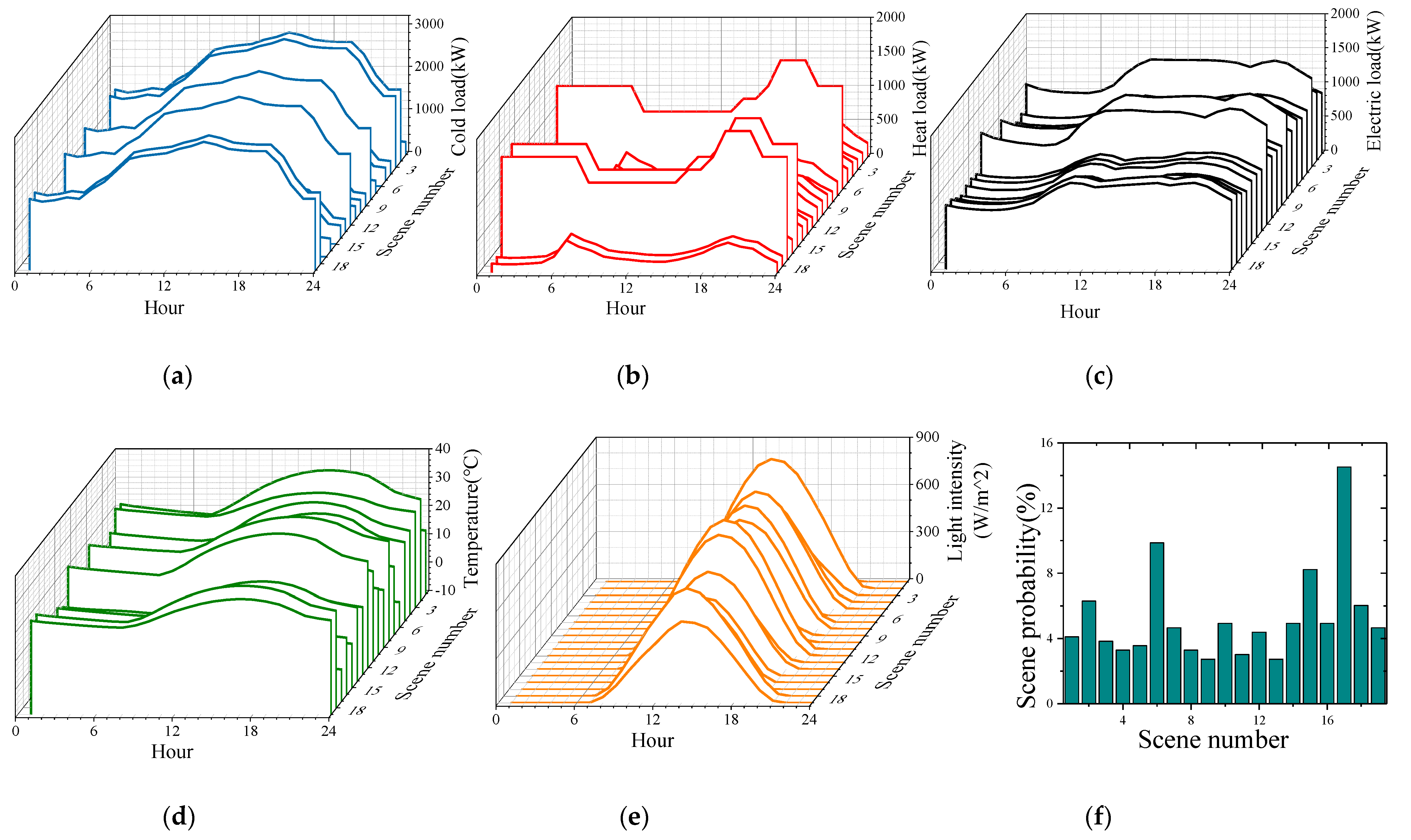
The probability of each clustering scene is shown in Table 1.
Figure 4 shows the change relationship curve among the comprehensive evaluation index, fuzzy coefficient m, and number of clusters c when clustering the three data groups of temperature, light intensity, and load.
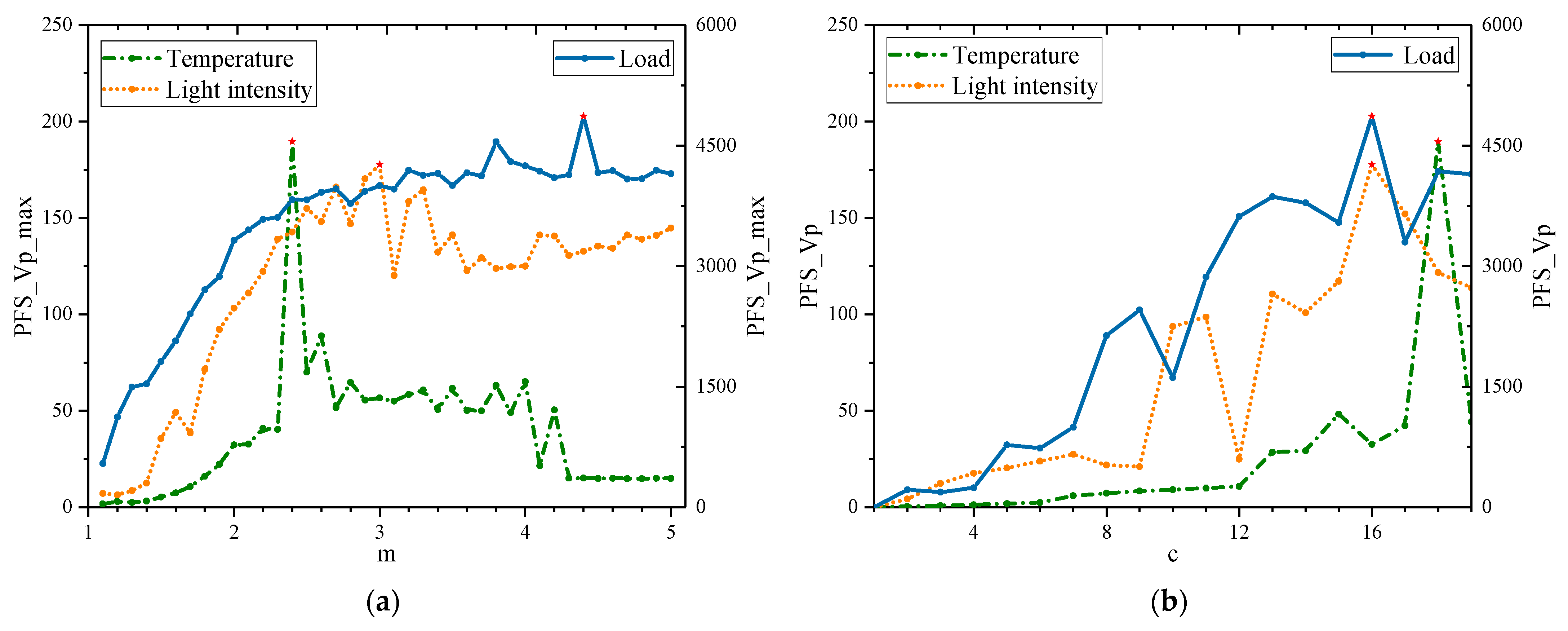
Figure 4a shows that, with an increase in fuzzy coefficient m, the maximum cluster comprehensive evaluation index of the three types of data presents a trend of first increasing and then falling. The best evaluation indexes of temperature, light intensity, and load appear at m = 2.4, 3, and 4.4, respectively. Figure 4b shows the change in the comprehensive clustering evaluation index of the three types of data with the number of clusters (c) under the optimal fuzzy coefficient. It could be seen that with the increase in cluster number c, the comprehensive evaluation index of clustering of the three types of data presents a changing trend, first rising and then falling, where k = 18, 16, and 16, respectively, correspond to the maximum values of the evaluation index. Combining the two figures, the clustering evaluation method based on the weighting of the PFS index and the Vp index is effective at clustering temperature, light intensity, and load. There is a maximum value of evaluation index for these three types of data, and the best fuzzy coefficient and cluster number can be found.
It can be seen from Figure 2 that temperature, light intensity, and load have obvious time series characteristics, and their values change regularly with changes in seasons and moments. This means that a small number of typical scenes can be found that can reflect the characteristics and laws of the overall data through scene clustering.
In order to further analyze the calculation process and mechanism of the improved FCM algorithm, the following gives the changes of the main parameters in the algorithm when the improved FCM algorithm is applied to cluster the light intensity data.
(1)
Set m = 1.1.
(2)
Keep the value of m unchanged, and calculate c = 2,3, …19, using the traditional FCM algorithm to cluster the light intensity dataset, and the clustering results are recorded as S2, S3, …S19.
(3)
Calculate the PFS indexes y_PFS2, y_PFS3, …y_PFS19, and Vp indexes y_Vp2, y_Vp3, …y_Vp19 of S2, S3…S19, respectively. When m = 1.1, the PFS index and Vp index are shown in Table 2.
(4)
Taking the vector Y_PFS = [y_PFS2, y_PFS3, …y_PFS19], Y_Vp = [y_Vp2, y_Vp3, …y_Vp19] as input, calculate the index weight according to the entropy weight method described in Section 2.3. When m = 1.1, the weight w1 = 0.356382547, w2 = 0.643617453.
(5)
Calculate the comprehensive evaluation index according to the weight, such as y_PFS_Vp2= w1* y_PFS2+ w2* y_Vp2. When m = 1.1, the PFS_Vp index is shown in Table 2.
(6)
m = m + 0.1. Repeat steps (2)–(5) until m is greater than 5 to stop the loop.
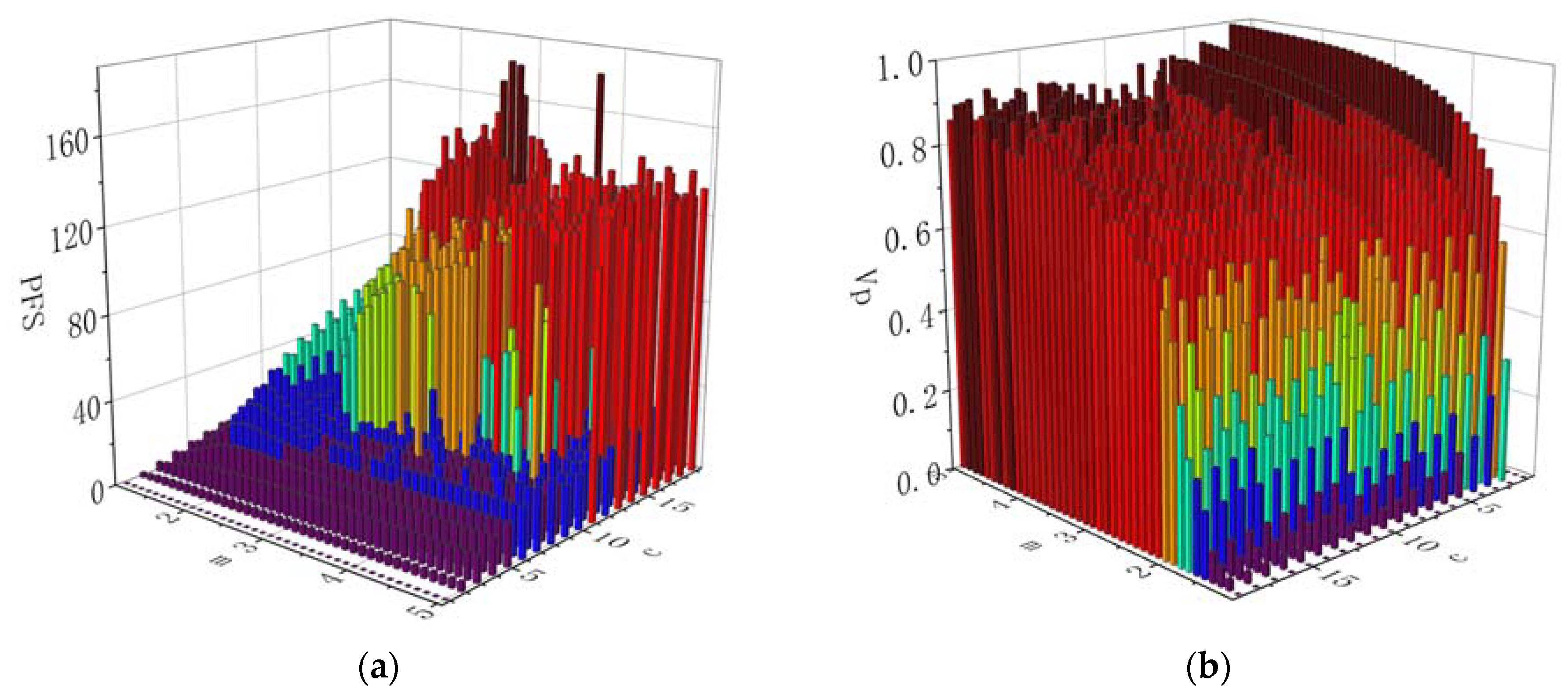
Figure 5 shows the PFS index and Vp index values of the clustering results under different fuzzy parameters m and the number of clusters c, respectively, obtained using traversal calculation.
It can be seen that the PFS index is more sensitive to changes in c than in m. In Figure 5a, when c is greater than 7, the PFS index increases rapidly. When c is greater than 15, the PFS index is always at a higher value, and the change in m hardly affects the PFS index. This is mainly because the PFS index focuses on the evaluation of the geometric result information of the clustering results, and the number of clusters directly affects the geometric structure of the clustering results. When the number of clusters increases, the intra-class distance of the clustering result will tend to decrease, and the inter-class distance will tend to increase. This also shows that the PFS index lacks evaluation ambiguity, and it is impossible to evaluate the effectiveness of the fuzzy clustering method alone. Therefore, it is necessary to introduce an index to evaluate ambiguity.
Figure 5b shows the Vp index value of the clustering results under different fuzzy parameters and the number of clusters. Contrary to the PFS index, the Vp index is almost exclusively affected by the fuzzy coefficient and is extremely insensitive to the number of clusters. This is because the Vp index only considers the membership degree information of the clustering results when constructing, and it is impossible to comprehensively evaluate the quality of the clustering results. In addition, it can be seen that when m is less than 2, the impact on the Vp index is greater. When m is greater than 2, the Vp index is always at a higher value. This will directly affect the distribution of indicator weights.
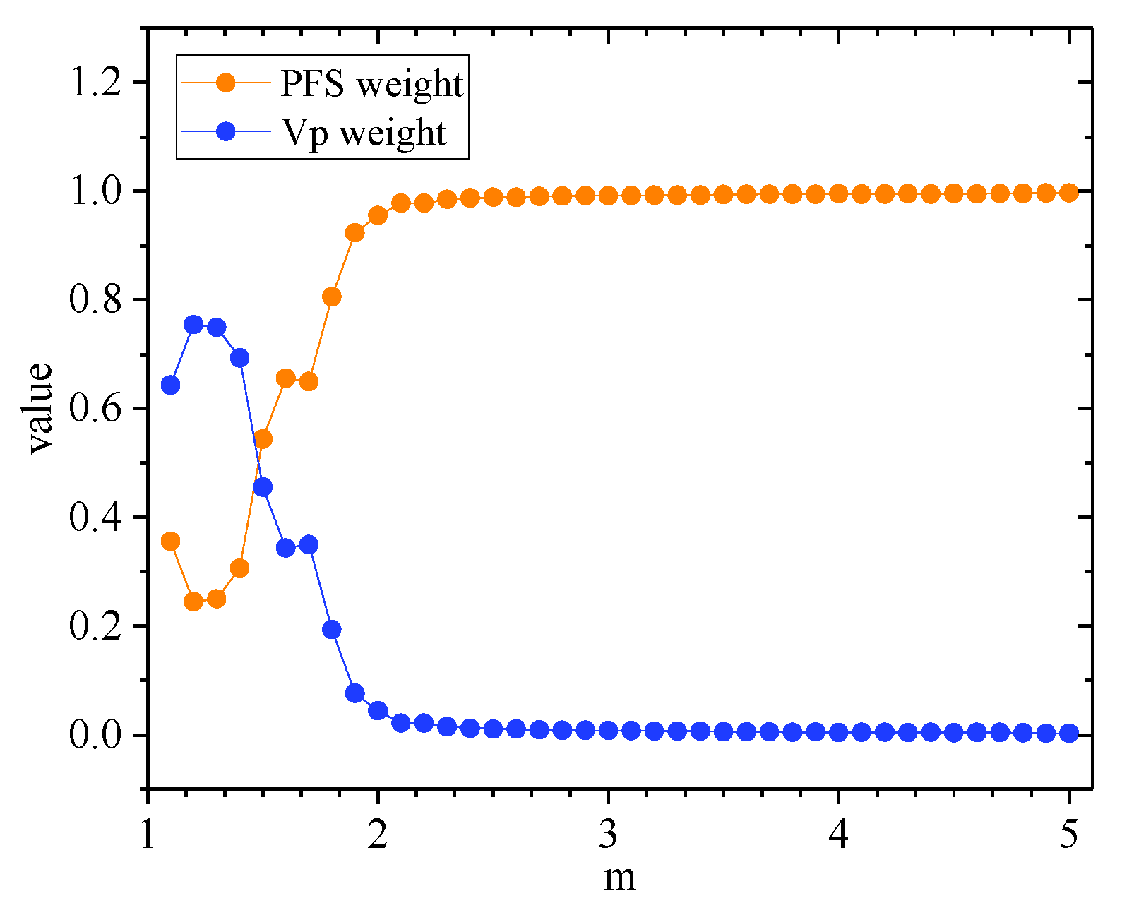
Figure 6 shows the two index weights obtained by using the entropy weight method under different fuzzy coefficients.
It can be seen from the figure that when m is less than 2, the weight of the Vp index is greater. However, when m is greater than 2, the weight of the Vp index tends to be almost zero. This is because the entropy method is an objective weight calculation method that assigns weights according to data distribution. When m is less than 2, the Vp index changes drastically with the change in m, which has a greater impact on the selection of the best parameters. Therefore, the weight obtained by the entropy method is larger. When m is greater than 2, the value of Vp index is not much different under different m and c, which is of little significance for the selection of the best parameter. Therefore, the assigned weight is smaller. On the contrary, the weight of the PFS index starts to be smaller, and gradually increases with the increase in m.
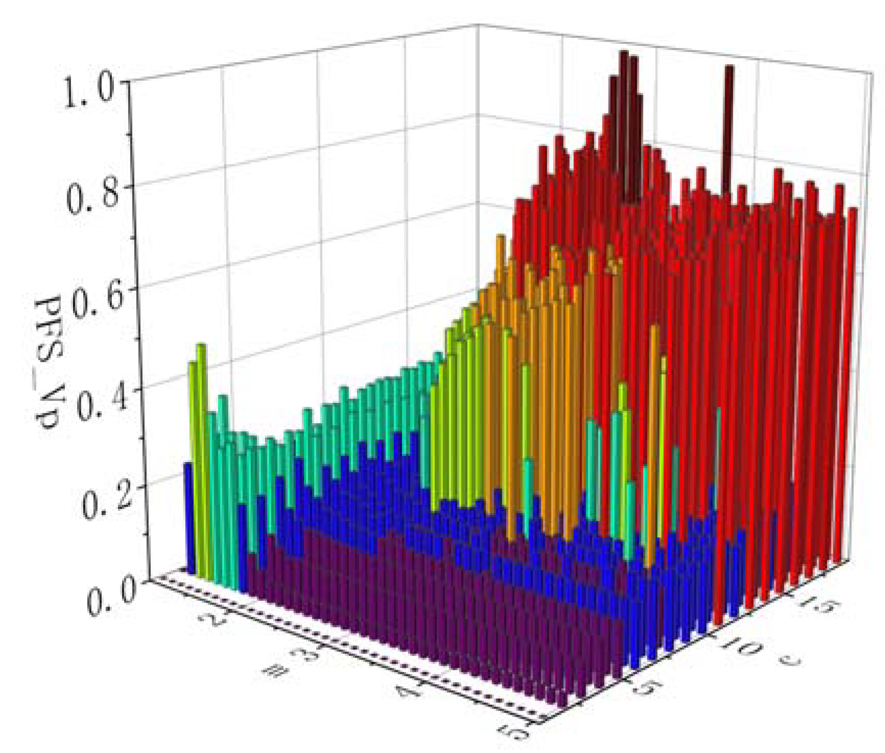
The PFS index and the Vp index are divided by their respective maximum values, so that the value of each PFS index and the Vp index is between 0 and 1. The purpose of this is to make the values of these two indicators have the same size benchmark. After that, the two indicators are weighted according to the weights determined using the entropy method. The obtained comprehensive clustering effectiveness evaluation index PFS_Vp is shown in Figure 7.
Comparing Figure 5 and Figure 7, it can be seen that PFS_Vp and PFS are roughly the same where m and c take larger values. Only when m and c are small can we see the effect of Vp on PFS_Vp. This is mainly due to the selection of weights.
From the above analysis, it can be seen that it is reasonable to introduce the PFS index and Vp index to comprehensively evaluate the clustering results in this paper. The focus of the evaluation of these two types of indicators is different. The objective weight selection through the entropy weight method can more comprehensively evaluate the pros and cons of fuzzy clustering results.

3. The Mathematical Model of the CCHP System

3.1. System Structure

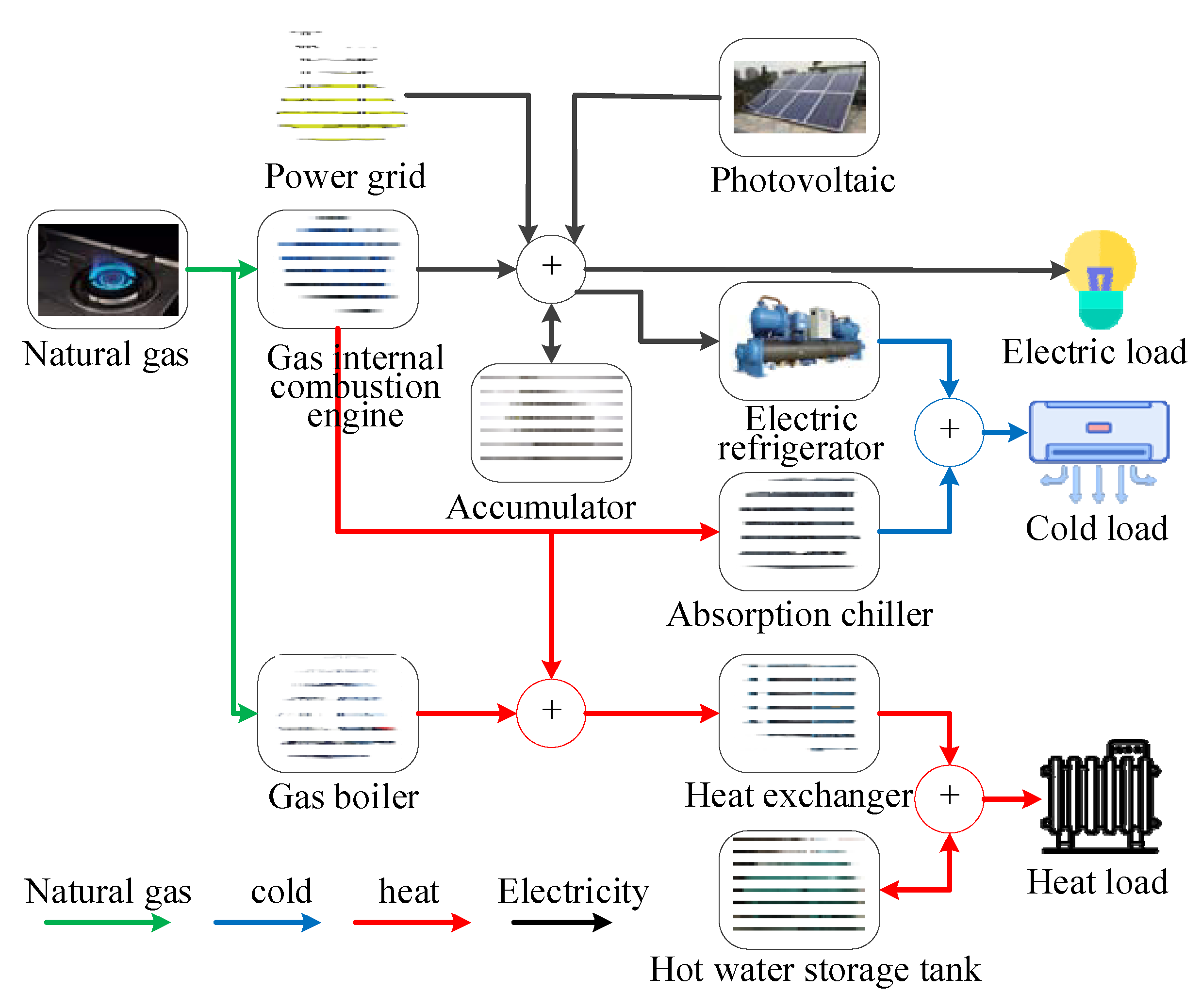
Figure 8 shows a diagram of a typical CCHP microgrid structure. In the figure, a micro turbine is shown that uses natural gas as fuel to provide electricity to users. At the same time, the high-temperature flue gas and the heat carried by the jacket water can be transported to the absorption chiller and heat exchange device to meet a user’s cold and heat load requirements.
In addition, photovoltaics, storage batteries, and urban power grids also participate in electrical energy supply. The heat storage tank can perform heat storage and release operations as required. Gas boilers and electric refrigeration units can supplement heating and cooling.

3.2. Micro Turbine

The micro turbine is the main energy supply equipment of the system and its operating efficiency varies greatly under different load rates. The mathematical model is as follows [4,40]:
{ V mt = t = 1 n P mt ( t ) Δ t η mtP ( t )L gas Q mt ( t )= P mt ( t ) η mtQ ( t ) η mtP ( t ) P mt min P mt ( t ) P mt max Q mt min Q mt ( t ) Q mt max
where V mt is natural gas consumption, m 3 . P mt ( t )  is the output electric power, kW.  is the waste heat power, kW. η mtP ( t ) and η mtQ ( t ) are power generation efficiency and waste heat efficiency, respectively. L gas is the calorific value of natural gas. In this paper, L gas takes the low calorific value of natural gas 9.7 ( kW h ) / m 3 . Δ t is the scheduling time scale, and this value takes 1 h.
Taking MWM’s TCG2016 V16C micro gas turbine as an example, according to actual test data, using MATLAB to perform polynomial curve fitting, the functional relationship between power generation efficiency, waste heat efficiency, and the load factor can be obtained as follows.
{ η mtP ( t ) = - 0.1040 ( P mt ( t ) P mt 0 ) 2 + 0.2260 ( P mt ( t ) P mt 0 ) + 0.2850 η mtQ ( t ) = 0.0960 ( P mt ( t ) P mt 0 ) 2 - 0.2480 ( P mt ( t ) P mt 0 ) + 0.6250 ,
where P mt 0 is the rated power of the micro turbine, kW.

3.3. Absorption Refrigeration Unit and Electric Refrigeration Unit

The mathematical model of the absorption chiller is as follows [41]:
{ Q ac = COP ac Q ac _ in Q ac min Q ac Q ac max ,
where Q ac is the cooling power, kW. Q ac _ in is the input heat power, kW. COP ac is the coefficient of refrigeration.
The relationship between the cooling power of an electric refrigerator and the power consumption is [41]
{ Q ec = COP ec P ec Q ec min Q ec Q ec max ,
where Q ec is the cooling power, kW. P ec is the power consumption, kW. COP ec is the energy efficiency ratio.

3.4. Photovoltaic Panel

The power output of photovoltaic cells is related to light intensity and ambient temperature [42]:
P pv = P STC G ( 1 + k pv ( T c 25 ) ) / 1000 ,
where P pv is photovoltaic power, kW. G is the light intensity, W m 2 . P STC is the maximum test power under standard test conditions, kW. k pv is the power temperature coefficient, %/°C. T c is the working temperature of the battery panel, and this value can be measured by ambient temperature T r .
T c = T r + 30 G / 1000 ,

3.5. Battery and Thermal Storage Tank

The mathematical model of energy storage devices, such as batteries and heat storage tanks, is [43]:
{ S s ( t ) = ( 1 - τ s ) S s ( t - 1 ) + ( P s , chr ( t ) η s , chr - P s , dis ( t ) η s , dis ) Δ t P s , chr min P s , chr P s , chr max P s , dis min P s , dis P s , dis max ε s min S sN min S s ε s max S sN max ,
where S s ( t ) is the remaining energy of the energy storage device during t period, kWh. P s , chr ( t ) and P s , d i s ( t ) are the input and output power of energy storage in t period, kW. τ s is the loss coefficient of energy storage. η s , chr and η s , dis are the energy input and output conversion efficiency of energy storage, respectively.

3.6. Gas Boiler and Heat Exchanger

The mathematical model of gas boiler and heat exchange device is as follows [43]:
{ Q ex = η ex Q ex _ in V gb ( t ) = Q gb ( t ) Δ t / ( η gb L gas ) Q ex min Q ex Q ex max Q gb min Q gb Q gb max ,
where Q ex _ in is the input heat power of the heat exchanger, kW. Q ex is the output heat power of the heat exchanger, kW. Q gb is the heating power of the gas boiler, kW. V gb is the gas consumption of gas boiler, m 3 . η gb and η ex are the efficiency of the gas boiler and heat exchanger, respectively.

3.7. System Energy Flow

According to the microgrid structure and the mathematical model of each device, the energy flow calculation model is constructed as follows:
{ Q ac = P mt ( η mtQ / η mtP ) k mt COP ac Q ec = Q load . c - Q ac Q ex = P mt ( η mtQ / η mtp ) ( 1 - k mt ) η ex Q gb = Q load . h - Q ex - Q hs P ec = Q ec / COP ec P op = k op P mt P grid = P load + P ec + P op - P mt - P es - P pv ,
where k mt is the proportion of the waste heat of the micro turbine distributed to the absorption chiller for refrigeration. Q load . c and Q load . h are, respectively, the values of cold and heat load, kW. P load . c is the value of the electrical load other than the power consumption of the electric refrigerator, kW. P op is the system’s own electric power, kW. k op is the system’s own electricity consumption rate, kW. P grid is the power purchased by the grid, kW. Q hs is the heat release power of the heat storage tank, kW. P es is the battery discharge power, kW. P pv is the photovoltaic output power, kW.

4. Bi-Level Optimization Configuration Model

4.1. Outer Configuration Optimization Model

4.1.1. Decision Variables and Objective Function

The outer layer optimization model takes the rated installation capacity of the photovoltaic, the rated installation capacity and the rated maximum charge and discharge power of the battery, and the rated installation capacity of the thermal storage tank as the optimization variables. Each objective and its function expression are as follows.
Objective 1: Annual conversion investment cost and annual operation and maintenance cost are minimized.
min f 1 = y in + s = 1 k ( 365 P s t = 1 T y op , s t ) ,
where y in is the annual conversion investment cost of the microgrid. k is the total number of scenes. T is the number of time periods divided in a day. y op , s t is the operating cost of the microgrid at time t in the s scenario, in yuan.
The specific expression of annual conversion investment cost is as follows:
y in = [ ( p esN k esp + E esN k esE ) n xt L es + E hsN k hs + p pvN k pv ] l ( 1 + l ) n xt ( 1 + l ) n xt 1 ,
where p pvN and E hsN are the rated installation capacities of photovoltaic and thermal storage tanks, kW, kWh. p esN and E esN are the maximum charge and discharge power and rated installation capacity of the battery, kW, kWh. k pv and k esE are the unit capacity cost of photovoltaic and thermal storage tank, yuan/kW. k esp , k esE , L es are the unit power cost, unit capacity cost and service life of the battery, yuan/kW, yuan/kWh. n xt is the planned service life of the system, in years. l is the discount rate.
Objective 2: Minimum annual carbon dioxide emissions f 2 .
min f 2 = s = 1 k ( 365 P s t = 1 T [ F co 2 , gas ( t , s ) + F co 2 , grid ( t , s ) ] ) ,
where f 2 is the total carbon dioxide emissions of the system, kg. P s is the scene probability. F co 2 , gas ( t , s ) and F co 2 , grid ( t , s ) are, respectively, the carbon dioxide emissions produced by gas and the equivalent carbon dioxide emissions of the electricity purchased by the power grid, kg. For a certain scene, the calculation formula is as follows:
{ F co 2 , gas ( t ) = K co 2 , gas V gas ( t ) F co 2 , grid ( t ) = K co 2 , grid P grid ( t ) Δ t
where K co 2 , gas and K co 2 , grid are the carbon dioxide conversion coefficient of natural gas and utility power, kg / Nm 3 , kg/kWh.

4.1.2. Restrictions

Taking the actual conditions of funds, venues, etc., into account, the construction of microgrids has the following restrictions:
{ P pvN min P pvN P pvN max P esN min P esN P esN max E esN min E esN E esN max E hsN min E hsN E hsN max ,

4.1.3. Solving Algorithm and Multi-Attribute Decision Making

The optimization configuration model of the upper microgrid constructed in this section is a multi-objective nonlinear model. For this model, the NSGA-II is used to solve the model.
The solution result of the multi-objective problem is a series of Pareto solutions. In this paper, the fuzzy multiple attribute decision-making method is used to select the best compromise solution. The specific formula is as follows [38]:
{ μ j k = ( f j max f j k ) / ( f j max f j min ) μ k = ( j = 1 n μ j k ) / ( k = 1 m j = 1 n μ j k ) o p t = { o | μ o = max ( μ k ) } ,

4.2. Inner Operation Optimization Model

4.2.1. Decision Variables and Objective Function

The inner optimization model is established on the basis of the capacity configuration of each device in the microgrid given by the outer model. The power generation of the micro turbine, the ratio of waste heat distribution, the charge and discharge power of the battery, and the heat storage and release power of the heat storage tank are selected as the optimization variables at various times of the day, and the daily operation and maintenance costs of the system are minimized as the goal. The function expression is as follows:
min y op = s = 1 k ( P s t = 1 T [ F gas ( t , s ) + F g r i d ( t , s ) + F op ( t , s ) ] ) ,
where f 1 is the total operating cost of the system, in yuan. P s is the probability of scene s. T is the period of the scheduling period. k is the number of scenes. F gas ( t , s ) , F g r i d ( t , s ) and F op ( t , s ) are, respectively, the system fuel cost, grid power purchase cost, and operation and maintenance cost in t period under the s scenario, in yuan. The specific expression for a certain scene is as follows:
{ F gas ( t ) = C gas [ V mt ( t ) + V gb ( t ) ] F grid ( t ) = C grid ( t ) P grid ( t ) Δ t F op ( t ) = C mt P mt ( t ) + C pv P pv ( t ) + C ac Q ac ( t ) + C ex Q ex ( t ) + C ec Q ec ( t ) + C es | P es ( t ) | + C hs | Q hs ( t ) | ,
where C gas and C grid are the price of natural gas and electricity, yuan / m 3 . C mt , C pv , C ac , C ec , C ex , C es and C hs are the operation and maintenance costs of micro turbine, photovoltaic, absorption chillers, electric chillers, heat exchangers, batteries, and heat storage tanks, yuan/kW.

4.2.2. Constraints and Solving Algorithms

The operating constraints of each device are as follows:
{ 0 P pv P pvN 0 P es , chr P e s , c h r . m a x 0 P es , dis P es , dis . max E esN θ es . min E es E esN θ es . max E hsN θ hs . min E hs E hsN θ hs . max ,
where P e s , c h r . m a x and P es , dis . max are the maximum charging and discharging power of the battery, kW. θ es . min and θ es . max are the ratio of the minimum and maximum load capacity of the battery.
The energy balance constraint expression is as follows:
{ P p v ( t ) + P m t ( t ) + P g r i d ( t ) + P e s . c h r ( t ) = P L ( t ) + P e c ( t ) + P o p ( t ) + P e s . d i s ( t ) Q e x ( t ) + Q g b ( t ) + Q h s . c h ( t ) Q l o a d . h ( t ) + Q h s . c h ( t ) Q a c ( t ) + Q e c ( t ) Q l o a d . c ( t ) ,
The optimization operation model of the inner microgrid constructed in this section is a nonlinear optimization model. For this model, this paper uses the PSO algorithm to solve it.

4.3. Model Flow Chart

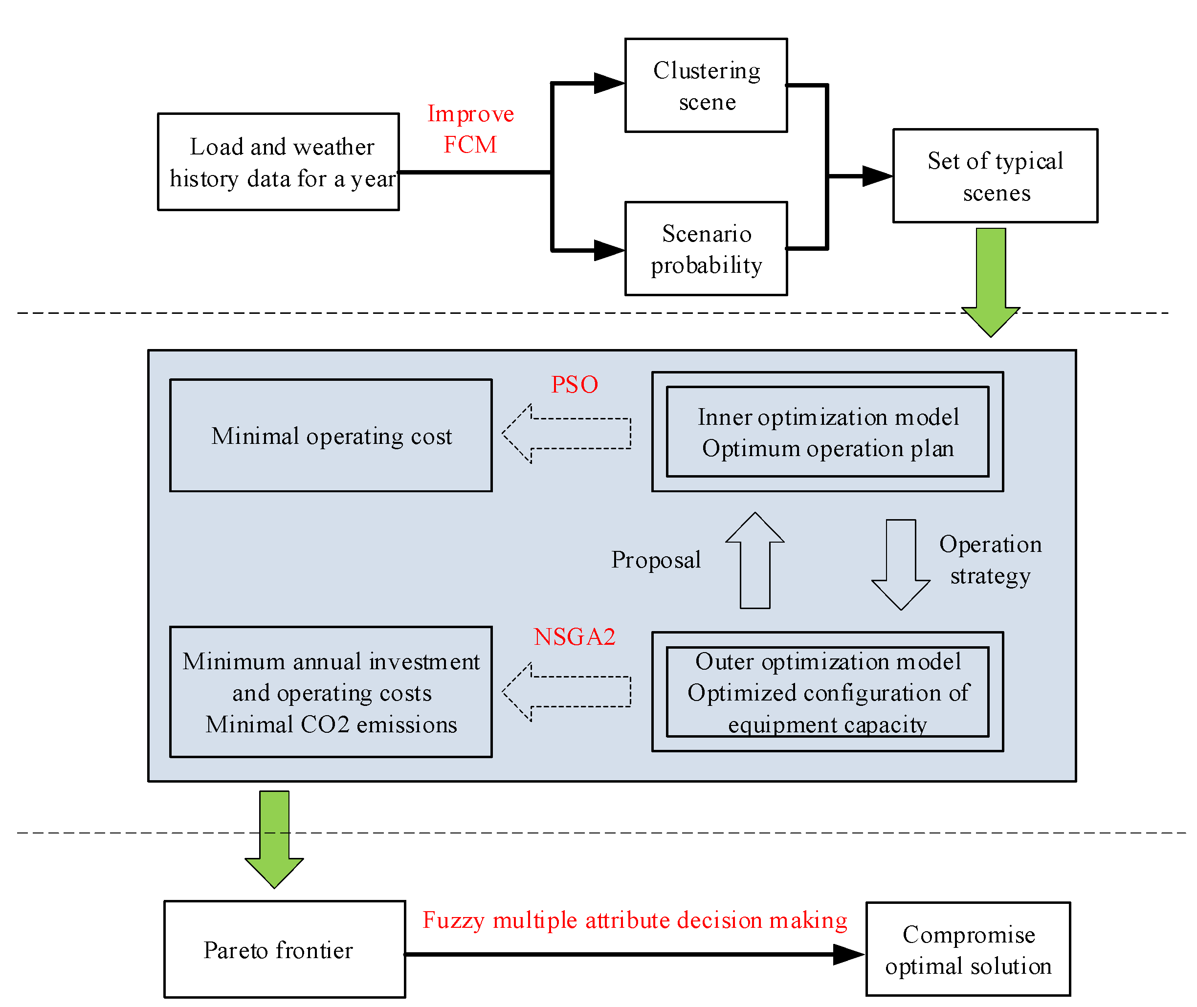
The calculation process of the CCHP bi-level optimization configuration model proposed in this paper is shown in Figure 9.
First, the improved FCM algorithm is used to cluster meteorological data such as temperature, light intensity, and cold, heat, and electrical load data on a monthly basis to obtain typical scenarios. After that, the bi-level optimal configuration model is constructed and solved. Finally, after the model is solved and the Pareto front obtained, the fuzzy multi-attribute decision-making method is used to select the best compromise solution.
The bi-level model’s solution process is: First, the outer model randomly generates a population and sends it to the inner model. Second, the inner model uses the PSO algorithm to solve the optimal operation plan based on the equipment capacity information input from the outer layer and returns it to the outer model according to the weather and load data. Third, the outer model performs non-dominated sorting and crowding calculation according to the operation plan returned by the inner model, and performs selection, crossover, and mutation to generate a new population. Finally, the new population is sent to the inner model for cyclic iterative calculation. When the number of iterations reaches a specified value, the loop stops, and the final generation population is output.

5. Case Analysis

5.1. Description of the Problem

Taking the Westin Hotel in Xi’an, China, as an example, the methods described in this paper are used to optimize the configuration of electricity, thermal energy storage, and photovoltaics to achieve maximum economy and environmental protection. The hourly load and weather data for the hotel in 2019 are shown in Section 2.5 The existing CCHP system parameters of the hotel are shown in Table 3.
Currently, the Westin Hotel CCHP system does not have electricity, thermal energy storage, and photovoltaic installations. The energy storage device can effectively suppress the fluctuation in the load, and realize the decoupling of energy production and consumption in time, thereby effectively solving the contradiction of energy supply and demand mismatch. Photovoltaic power generation is clean, environmentally friendly, and economical, which can reduce the cost of power supplies in hotels. To improve the comprehensive operating benefits of the hotel’s CCHP system, this paper will use the proposed method to equip it with suitable capacity batteries, thermal storage tanks, and photovoltaics on the basis of existing equipment to maximize economic and environmental benefits.

5.2. Load and Weather Data Clustering Based on Improved FCM Algorithm

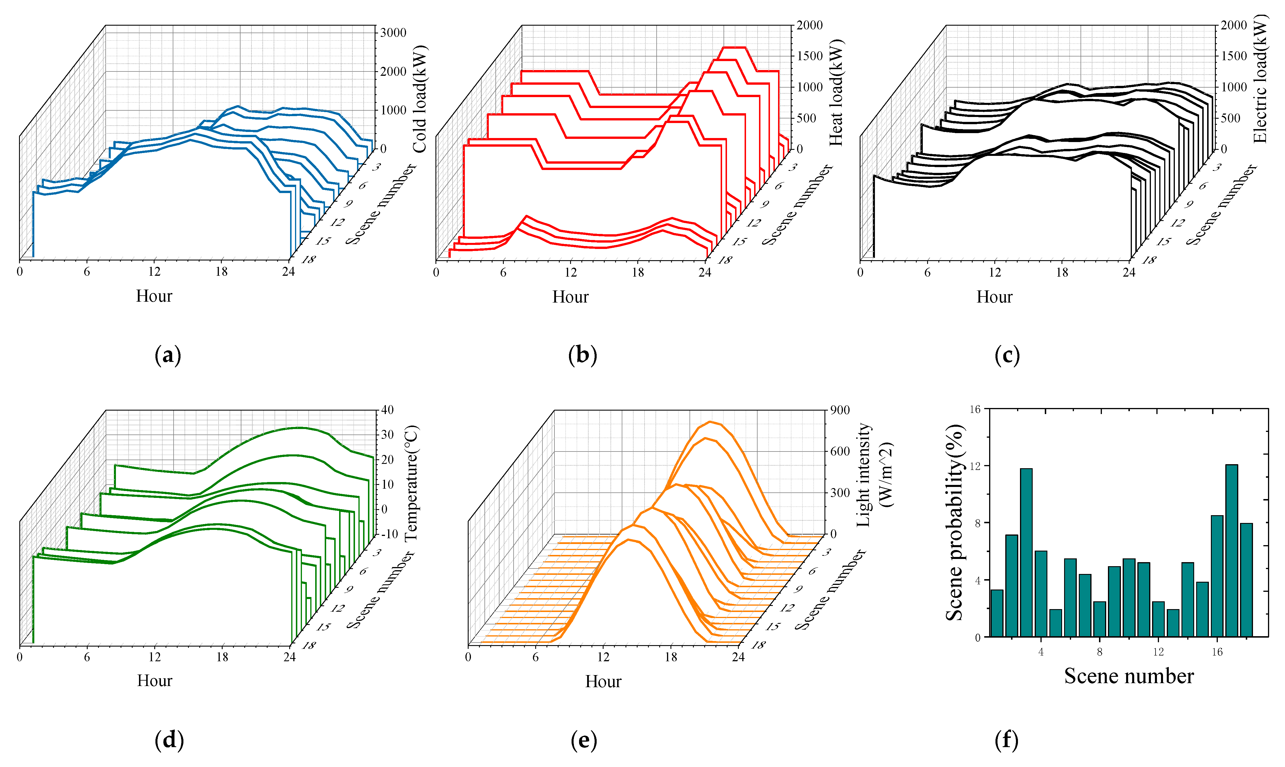
The 2019 Westin Hotel’s cold, heating, electrical load, temperature, and light intensity meteorological data is taken as a whole, and then the improved FCM algorithm described in Section 2.4 is used to progressively reduce the scene. The results of the reduction are shown in Figure 10.
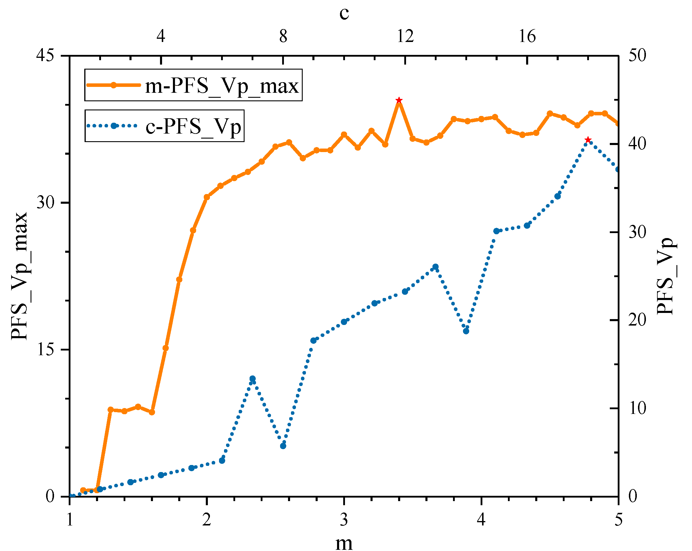
The relationship among the fuzzy coefficient, the cluster number, and the comprehensive evaluation index during the reduction process is shown in Figure 11.

5.3. Optimization Configuration Results

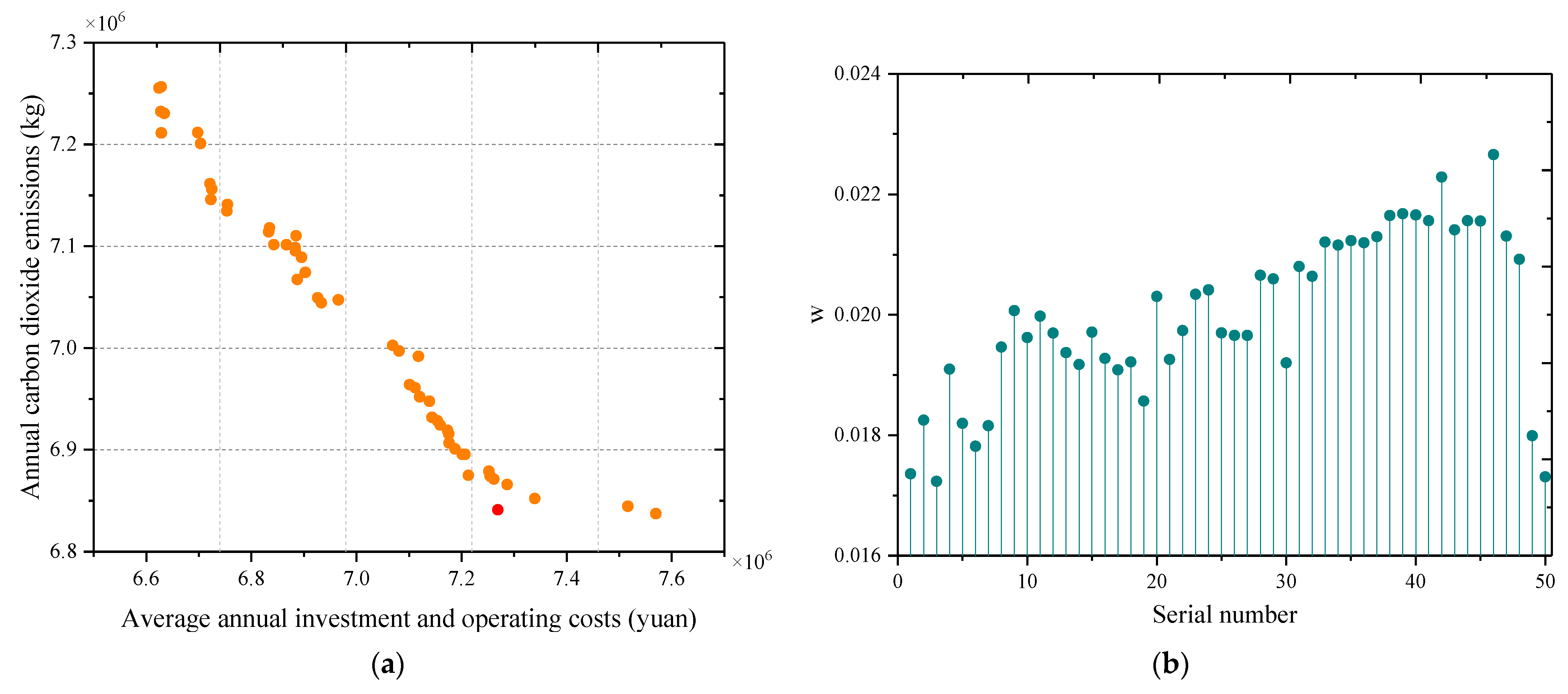
A bi-level optimal configuration model is constructed as described in Section 3, and the reduced scene is input into the model. The resulting Pareto frontier is shown in Figure 12. The resulting Pareto solution set is shown in Table 4.
It can be seen from Figure 12a that the average annual investment operating cost and the annual carbon dioxide emissions are contradictory, and there is no ideal optimal solution. According to the multi-attribute decision-making method described in Section 4.1.3, the comprehensive rating coefficient (w) of each scheme is calculated, as shown in Figure 12b. It can be seen from the figure that the solution of the No. 46 scheme has the largest w value, so the No. 46 solution was selected as the best compromise solution.

5.4. Analysis and Comparison

To verify the effectiveness of the method proposed in this paper, it is compared with the single-level optimization configuration model based on a given operation mode and the configuration model based on the traditional FCM clustering algorithm.

5.4.1. Compared with a Single-Tier Optimal Configuration Model Based on a Given Operating Mode

The bi-level optimization configuration model proposed in this paper is compared with the single-level optimization configuration model of the given operation mode in the literature [44]. The two commonly used operating modes are as follows.
(1)
Following the electrical load (FEL) mode. The gas generator set in the CCHP system determines its power generation capacity according to the building’s heat under the premise of not exceeding the design capacity. When the heat generated by the system does not meet the demand for cooling and heating loads, it is supplemented by electric refrigerators and electric boilers. When the power generated by the system does not meet the electrical load demand, it is supplemented by the external grid. Since there is no excess heat problem in the system’s operating mode at this time, the energy storage device is not considered.
(2)
Following the thermal load (FTL) mode. The gas generator set of the CCHP system determines its power generation capacity according to the electrical load required by the building under the premise of not exceeding its design capacity. When the power generated by the system does not meet the electrical load demand, it is supplemented by the external grid. When the system generates excess heat, the excess heat is stored in the energy storage device. When the heat generated by the system does not meet the demand for cooling and heating loads, it is first replenished by the energy storage device. If it is still not satisfied, it will be supplemented by an electric boiler and an electric refrigerator.
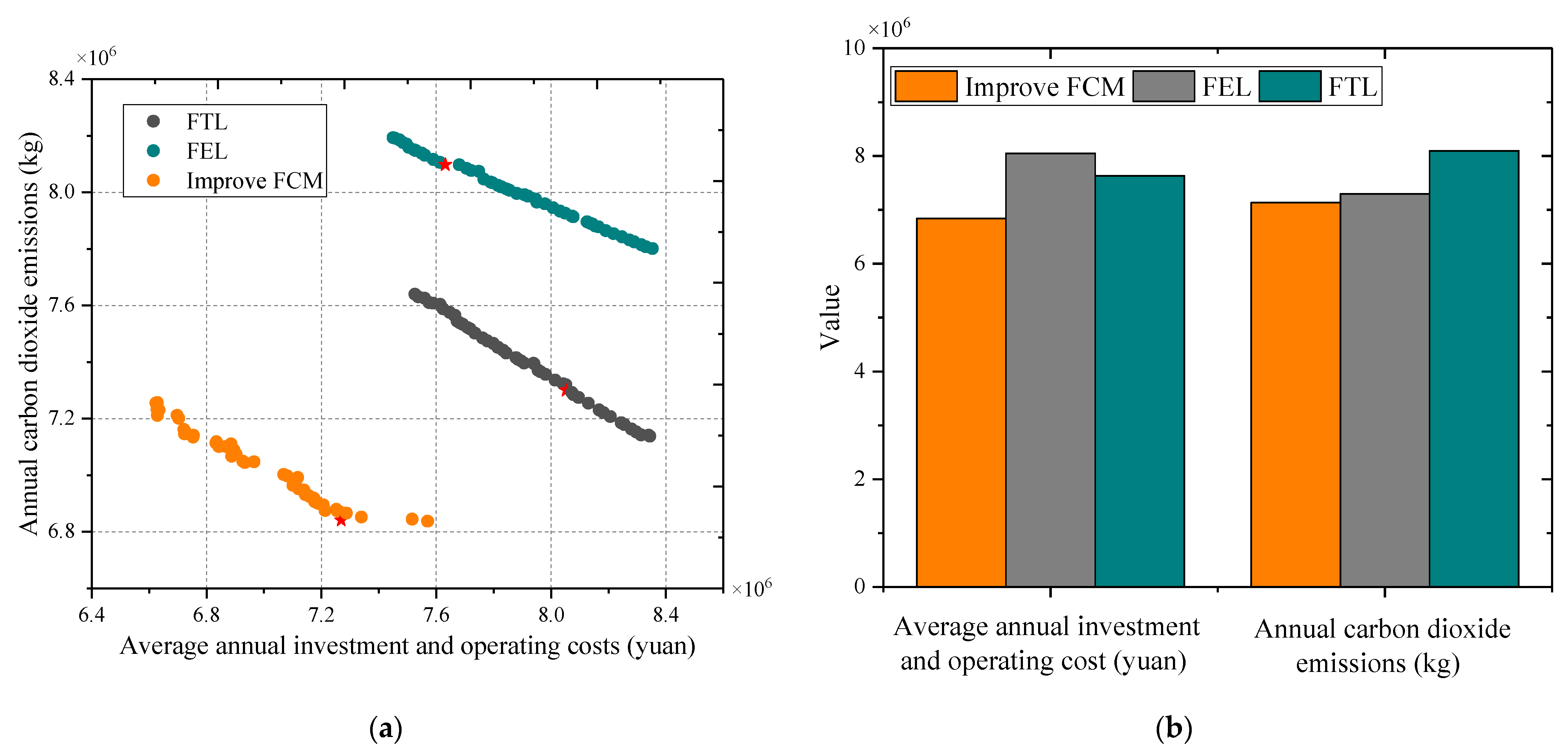
In addition to replacing the inner optimization operation model with a given operation mode, other processing methods of the single-layer optimization model include data clustering, the energy flow calculation model of the CCHP system, the construction of the outer model and the solving algorithm are the same as the two-layer optimization optimization model. The resulting Pareto solution set is shown in Figure 13.
It can be seen that the overall inferiority of the Pareto frontier obtained by the optimal configuration model under a given operating mode is the same as the method proposed in this article. The compromise solution selected from the Pareto solution set is shown in Figure 13b. It can be seen from the figure that the average annual investment and operating costs of the optimization configuration scheme obtained by the method proposed in this paper are 10.78% lower than the FEL model and 4.99% lower than the FTL model; the annual carbon dioxide emissions are 6.70% lower than the FEL model and 18.36% lower than the FTL model.

5.4.2. Compared with the Configuration Model Based on the Traditional FCM Clustering Algorithm

The traditional FCM algorithm is used to cluster the graph data. m = 2, and the cluster center is set to a maximum value of 19. The clustering results are shown in Figure 14.
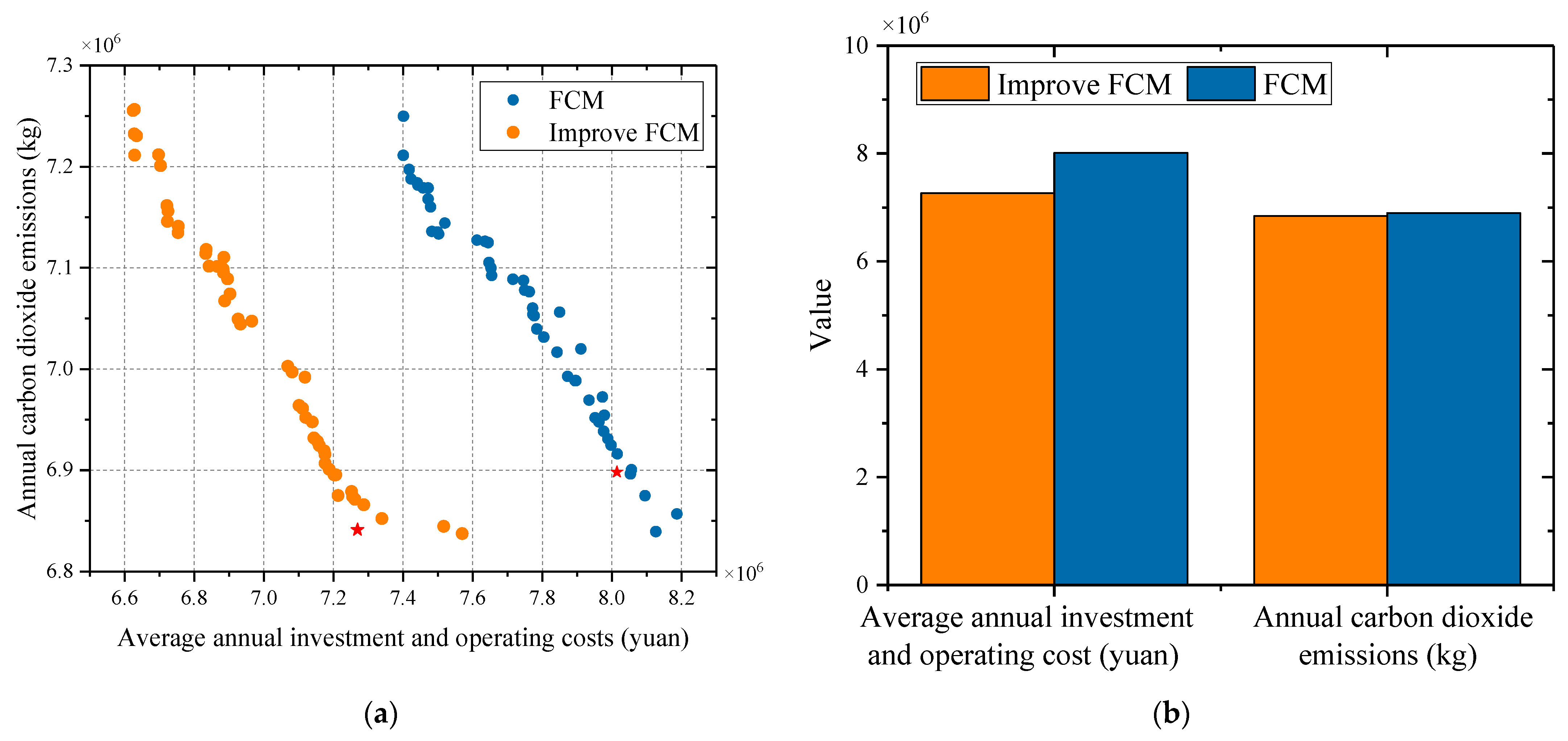
The obtained scene reduction is brought into the optimization model, and the results are shown in Figure 15.
It can be seen from Figure 15 that the Pareto frontier based on the configuration model of the traditional FCM clustering algorithm is, overall, still inferior to the method proposed in this article. As in the previous section, the compromise solution is selected from it. It can be calculated that the average annual investment and operating cost of the optimized configuration scheme obtained by the method proposed in this paper are reduced by 10.25% and the annual carbon dioxide emissions are reduced by 0.83%.
To further verify the superiority of the improved FCM clustering algorithm proposed in this paper compared with the traditional FCM clustering algorithm, in solving the problem of CCHP optimization configuration, this paper inputs the actual load and weather data from 2019, as well as the two optimized configuration schemes obtained, into the inner optimization operation model described in Section 4.2. Then the actual operating costs and carbon dioxide emissions are calculated under the two schemes.
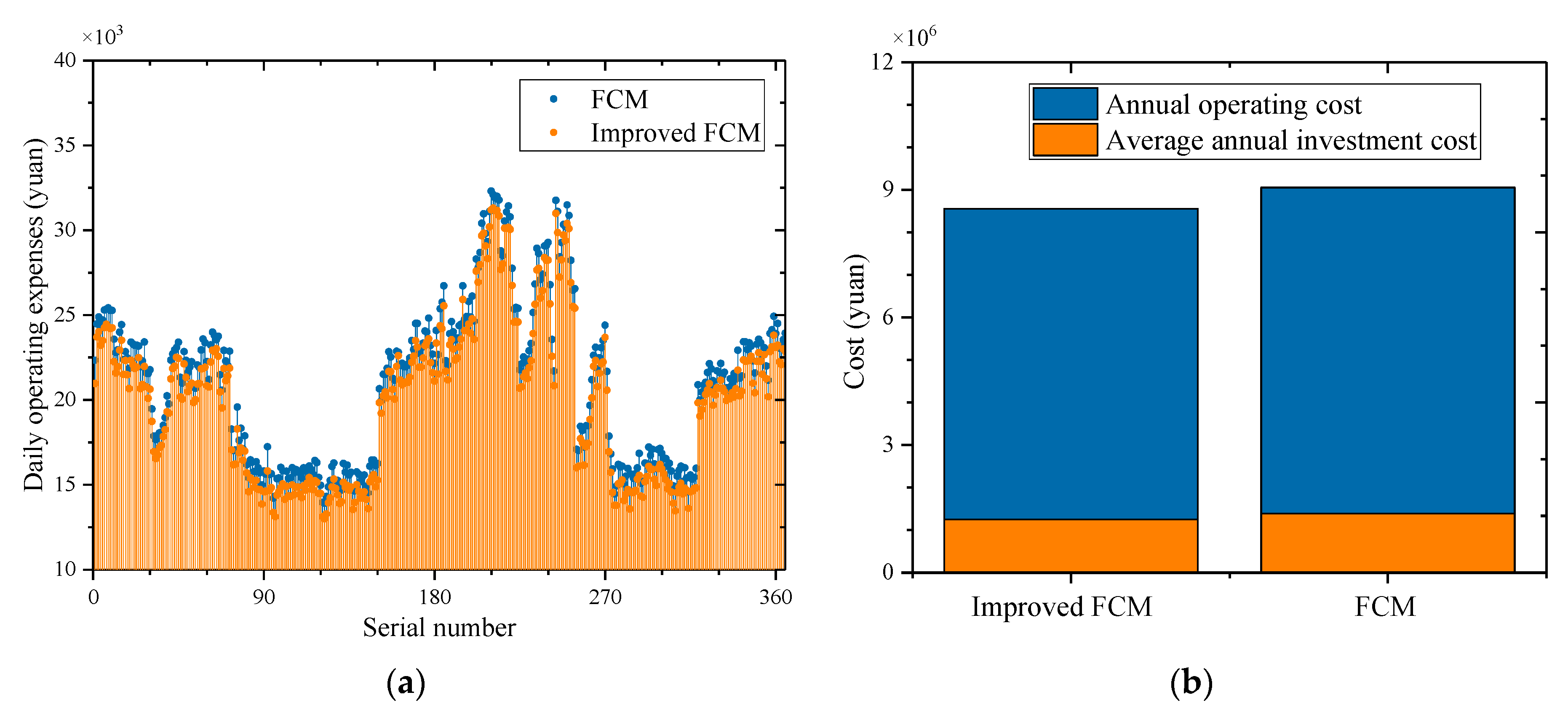
Figure 16 shows the daily operating cost and the total annual cost under the two configuration schemes.
It can be seen from Figure 16 that, in most cases, compared with the traditional FCM algorithm, the operating cost of the optimized configuration scheme obtained by applying the improved FCM algorithm is lower. The annual operating cost dropped by 358,962 yuan, with a drop rate of 4.68%. The average annual investment cost dropped by 140,090 yuan, and the rate of decrease was 10.07%. The total cost fell by 499,052 yuan, a rate of decrease of 5.51%.
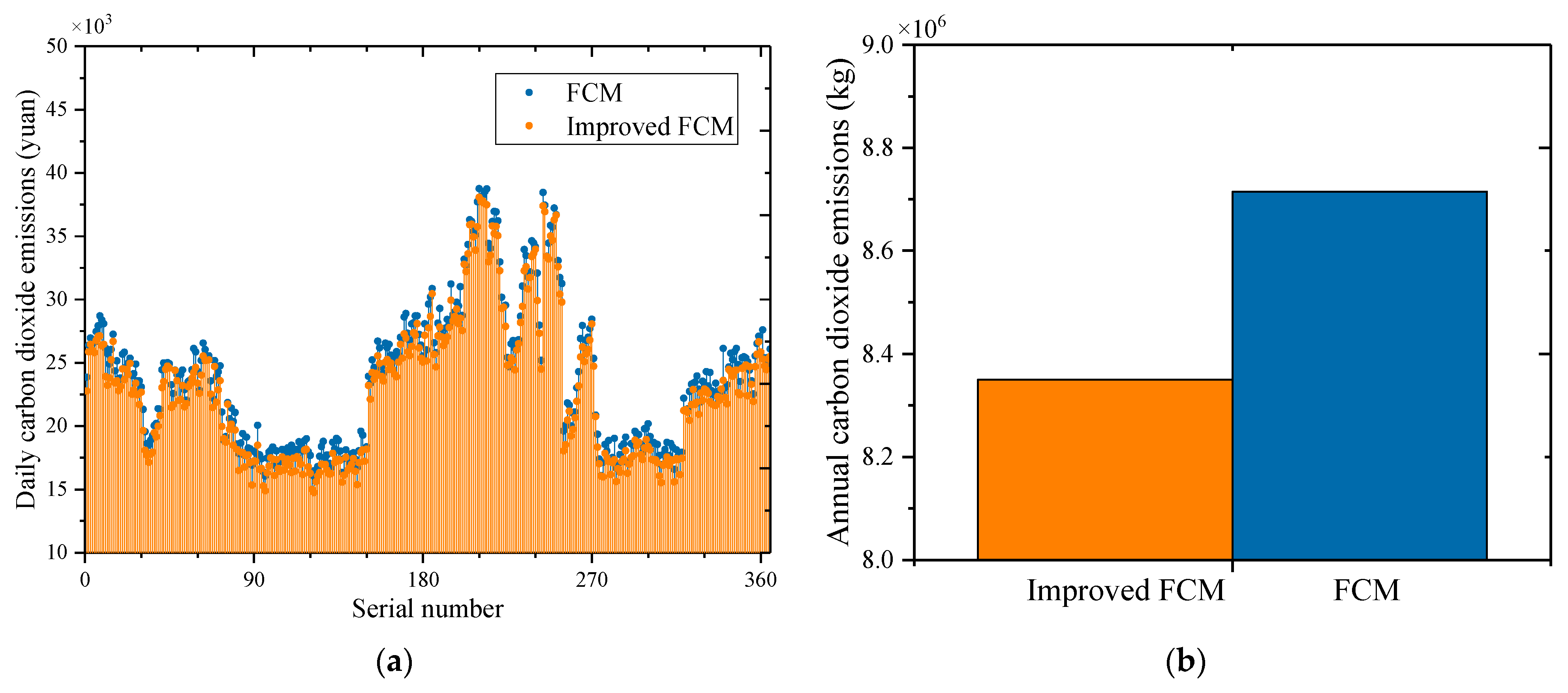
Figure 17 shows the daily carbon dioxide emissions and the total annual carbon dioxide emissions under the two configuration schemes.
It can be seen from Figure 17 that, in most cases, compared to the traditional FCM algorithm, the optimization configuration scheme obtained by applying the improved FCM algorithm has lower carbon dioxide emissions. The total emissions in three months fell by 365,065 kg, a decrease rate of 4.19%.
The analysis of the above examples fully shows that, in solving the problem of CCHP optimal configuration, compared with the traditional FCM clustering algorithm, the improved FCM clustering algorithm proposed in this paper has a better clustering effect. The method can better reflect the overall characteristics and laws of weather and load, so the configuration scheme obtained by the optimization model is more suitable in practice, and the economic and environmental protection of the CCHP system are improved.

5.4.3. Comparison of System Operating Costs before and after Optimized Configuration

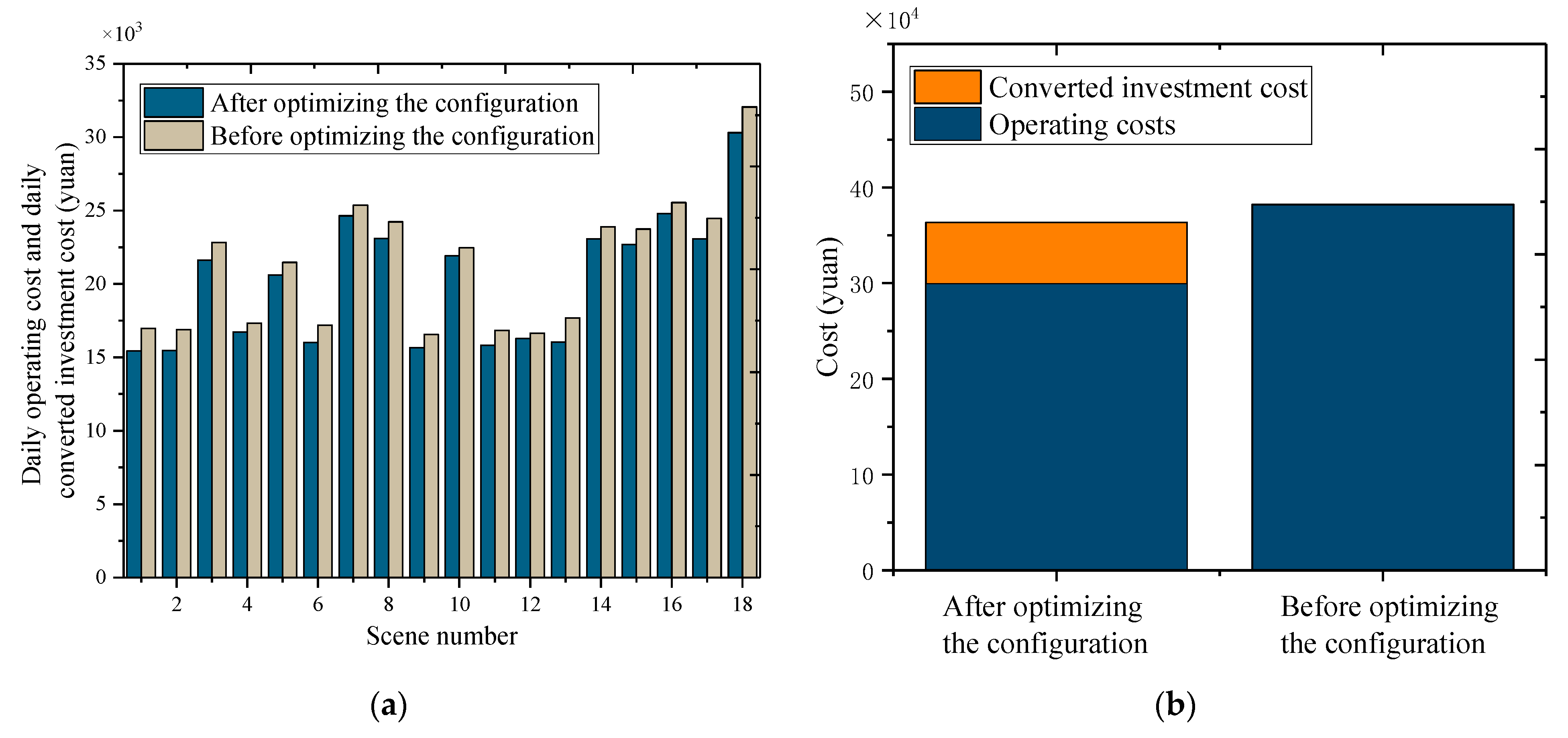
In order to verify the effectiveness of the optimized configuration of the system, this section compares the CCHP system without electricity, thermal energy storage devices, and photovoltaics with the optimized configuration. The operating costs of the two systems are calculated in 18 typical scenarios obtained by clustering. The calculation results are shown in Figure 18.
It can be seen from Figure 18a that the daily operating cost of the system after configuration in the 18 typical scenarios is less than the operating cost of the system before the configuration. This is mainly because the system can use sunlight to generate electricity after the optimized configuration, and the two energy storage devices of electricity and heat realize a reasonable adjustment of energy, avoiding a waste of energy. Figure 18b shows the total cost before and after the daily configuration of the 18 scenarios. Compared with before the configuration, the operating cost after configuration is reduced by 21.63%, and the increased equipment cost is allocated to each day, and the total cost after configuration is reduced by 4.95%.
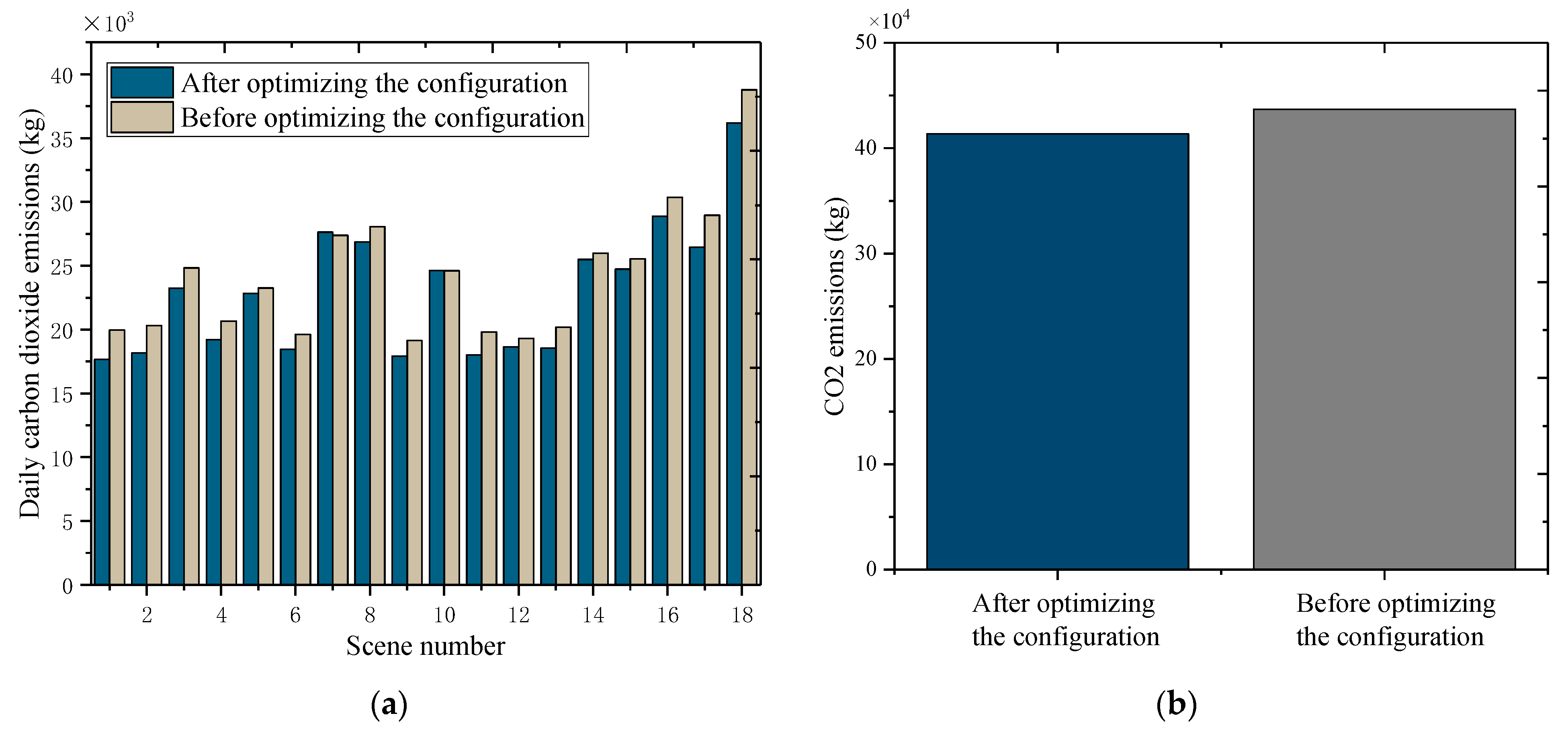
It can be seen from Figure 19a that the daily carbon dioxide emissions of the system after configuration in the 18 typical scenarios are all less than before the configuration. This is mainly because the optimized configuration of the system uses clean solar energy, which reduces the use of natural gas and city electricity. In addition, the energy storage device realizes reasonable energy adjustment and avoids energy waste. Figure 19b shows the total carbon dioxide emissions before and after the daily configuration of the 18 scenarios. Compared with before configuration, carbon dioxide emissions after the configuration are reduced by 5.31%.
By comparing the operation of the system before and after the configuration, it can be seen that it is necessary for the CCHP system to have a reasonable configuration of photovoltaics, and electric and thermal energy storage as it can significantly reduce system operating costs and carbon dioxide emissions, and better take advantage of the high energy efficiency, energy saving and environmental protection of the CCHP system.

6. Conclusions

To address the problem that the optimal fuzzy coefficients and the number of clusters are difficult to determine in the FCM algorithm, this paper introduces the PFS index to evaluate the geometric information of clustering results and the Vp index to evaluate the affiliation information based on the traditional FCM algorithm from the evaluation of clustering effectiveness. The optimal fuzzy coefficient and the number of clusters are found. The validity test of the improved algorithm shows that (1) the evaluation focus of PFS and Vp indicators are different. The PFS indicator is more sensitive to the number of clusters. The VP indicator is more sensitive to smaller fuzzy coefficients and extremely insensitive to the number of clusters. (2) The method of using the entropy weighting method to weigh PFS indicators and Vp indicators is effective. On the one hand, the evaluation effects of these two indicators can complement each other. On the other hand, the optimal fuzzy coefficients and the number of clusters that make the comprehensive evaluation index reach the maximum value are found in the clustering test on the actual data. In addition, the method of determining the optimal number of clusters and the optimal fuzzy coefficient proposed in this paper does not contain any subjective factors. The entropy weight method used to determine the weight is a completely objective method to determine the weight according to the law of data distribution.
Based on the improvement of the clustering algorithm, we constructed a bi-layer optimal configuration model for the optimal configuration problem of the CCHP system. The model takes the clustering results of load and meteorological data using the improved FCM algorithm as the input. The best CCHP system configuration solution is taken as the output. The algorithm analysis shows that the optimized configuration method obtained by the improved FCM algorithm is better than the traditional FCM clustering algorithm. This shows that the improved FCM algorithm is more suitable for load and weather scenario reductions for the CCHP system optimization configuration problem. It is able to find typical scenarios that are more consistent with the overall characteristics and variation patterns of load and meteorology.
The starting point of the improved FCM algorithm proposed in this paper is to better serve the problem of optimal configuration of the CCHP system. Algorithm analysis also verifies that the improved algorithm is effective for the results of this problem. However, whether the improved FCM algorithm is applicable to clustering random datasets without physical background needs further validation. In addition, both the PFS index and the Vp index are evaluation indices that perform better individually, but it cannot be determined if their combination is necessarily better than other possible combinations, which remains to be studied.

Author Contributions

Conceptualization, K.Z. and P.F.; methodology, K.Z.; software, P.F.; validation, K.Z., P.F. and G.Z.; formal analysis, K.Z.; investigation, X.H.; resources, G.Z.; data curation, J.H.; writing—original draft preparation, K.Z. and P.F.; writing—review and editing, K.Z., P.F. and G.Z.; visualization, T.X.; supervision, T.X.; project administration, G.Z.; funding acquisition, G.Z; investigation, X.H. All authors have read and agreed to the published version of the manuscript.

Funding

This research was funded by the Key Research and Development Plan of Shaanxi Province (2018-ZDCXL-GY-10-04), the Research Fund of the State Key Laboratory of Eco-Hydraulics in Northwest Arid Region, Xi’an University of Technology (2019KJCXTD-5).

Data Availability Statement

The study did not report any data.

Conflicts of Interest

The authors declare no conflict of interest.

Abbreviations

Variables
CCHPCombined Cooling, Heating and Power
FCMFuzzy C-means
PFSpseudo-F statistical ratio
NSGA-IINon-dominated Sorting Genetic Algorithm II
PSOParticle swarm optimization
FELFollowing the electrical load
FTLFollowing the thermal load
mthe fuzzy coefficient
cthe number of clusters
V mt natural gas consumption of the micro turbine
P mt the electric power output of the micro turbine
Q mt the waste heat power of the micro turbine
η mtP power generation efficiency of the micro turbine
η mtQ waste heat efficiency of the micro turbine
L gas the calorific value of natural gas
P mt 0 the rated power of the micro turbine
Q ac the cooling power of absorption refrigeration unit
Q ac _ in the input heat power of absorption refrigeration unit
COP ac the coefficient of absorption refrigeration unit
Q ec the cooling power of electric refrigeration unit
P ec the power consumption of electric refrigeration unit
COP ec the energy efficiency ratio of electric refrigeration unit
P pv photovoltaic power
Gthe light intensity
P STC the maximum test power under standard test conditions
k pv the power temperature coefficient
T c the working temperature of the battery panel
T r the ambient temperature
S es the remaining energy of battery
P es the input power of battery
S hs the remaining energy of heat storage tank
P hs the input power of heat storage tank
τ es the loss coefficient of battery
τ hs the loss coefficient of energy storage
η s , chr the energy input conversion efficiency of energy storage
η s , dis the energy output conversion efficiency of energy storage
Q ex the output heat power of the heat exchanger
Q ex _ in the input heat power of the heat exchanger
Q gb the heating power of the gas boiler
V gb the gas consumption of gas boiler
η gb the efficiency of gas boiler
η ex the efficiency of heat exchanger
k mt the proportion of the waste heat of the micro turbine distributed to the absorption chiller for refrigeration
Q load . c the value of cold load
Q load . h the value of heat load
P load the value of the electrical load other than the power consumption of the electric refrigerator
P op the system’s own electric power
k op the system’s own electricity consumption rate
P grid the power purchased by the grid
Q hs the heat release power of the heat storage tank
P es the battery discharge power
P pv the photovoltaic output power
y in the annual conversion investment cost of the microgrid
kthe total number of scenes
Tthe number of time periods divided in a day
y op , s t the operating cost of the microgrid at time t in the s scenario
p pvN the rated installation capacities of photovoltaic
E hsN the rated installation capacities of thermal storage tanks
p esN the maximum charge and discharge power
E esN the rated installation capacity of the battery
k pv the unit capacity cost of photovoltaic
k esE the unit capacity cost of thermal storage tank
k esp the unit power cost
k esE the unit capacity cost
L es the service life of the battery
n xt the planned service life of the system
l the discount rate
P s the scene probability
F co 2 , gas the carbon dioxide emissions produced by gas
F co 2 , grid the equivalent carbon dioxide emissions of the electricity purchased by the power grid
K co 2 , gas the carbon dioxide conversion coefficient of natural gas
K co 2 , grid the carbon dioxide conversion coefficient of utility power
C mt the operation and maintenance costs of micro turbine
C pv the operation and maintenance costs of photovoltaic
C ac the operation and maintenance costs of absorption chillers
C ec the operation and maintenance costs of electric chillers
C ex the operation and maintenance costs of heat exchangers
C es the operation and maintenance costs of batteries
C hs the operation and maintenance costs of heat storage tanks
P e s , c h r . m a x the maximum charging power of the battery
P es , dis . max the maximum discharging power of the battery
θ es . min the ratio of the minimum load capacity of the battery
θ es . max the ratio of the maximum load capacity of the battery

References

  1. Wang, J.; Lu, Z.; Li, M.; Lior, N.; Li, W. Energy, exergy, exergoeconomic and environmental (4E) analysis of a distributed generation solar-assisted CCHP (combined cooling, heating and power) gas turbine system. Energy 2019, 175, 1246–1258. [Google Scholar] [CrossRef]
  2. Gu, W.; Wu, Z.; Bo, R.; Liu, W.; Zhou, G.; Chen, W.; Wu, Z. Modeling, planning and optimal energy management of combined cooling, heating and power microgrid: A review. Int. J. Electr. Power Energy Syst. 2014, 54, 26–37. [Google Scholar] [CrossRef]
  3. Yang, G.; Zhai, X. Optimization and performance analysis of solar hybrid CCHP systems under different operation strategies. Appl. Therm. Eng. 2018, 133, 327–340. [Google Scholar] [CrossRef]
  4. Zhang, L.; Zhang, L.; Sun, B.; Zhang, C.; Li, F. Nested optimization design for combined cooling, heating, and power system coupled with solar and biomass energy. Int. J. Electr. Power Energy Syst. 2020, 123, 106236. [Google Scholar] [CrossRef]
  5. Wang, J.; Qi, X.; Ren, F.; Zhang, G.; Wang, J. Optimal design of hybrid combined cooling, heating and power systems considering the uncertainties of load demands and renewable energy sources. J. Clean. Prod. 2021, 281, 125357. [Google Scholar] [CrossRef]
  6. Afzali, S.F.; Mahalec, V.J.E. Optimal design, operation and analytical criteria for determining optimal operating modes of a CCHP with fired HRSG, boiler, electric chiller and absorption chiller. Energy 2017, 139, 1052–1065. [Google Scholar] [CrossRef]
  7. Zheng, L.; Wang, X.; Jiang, B. Multi-Objective Optimal Configuration of the CCHP System. Processes 2020, 8, 351. [Google Scholar] [CrossRef] [Green Version]
  8. Zhang, L.Z.; Li, F.; Sun, B.; Zhang, C.H. Integrated Optimization Design of Combined Cooling, Heating, and Power System Coupled with Solar and Biomass Energy. Energies 2019, 12, 21. [Google Scholar] [CrossRef] [Green Version]
  9. Wegener, M.; Malmquist, A.; Isalgue, A.; Martin, A.; Arranz, P.; Camara, O.; Velo, E. A techno-economic optimization model of a biomass-based CCHP/heat pump system under evolving climate conditions. Energy Convers. Manag. 2020, 223, 113256. [Google Scholar] [CrossRef]
  10. Zhu, X.Y.; Zhan, X.Y.; Liang, H.; Zheng, X.Y.; Qiu, Y.W.; Lin, J.; Chen, J.C.; Meng, C.; Zhao, Y.R. The optimal design and operation strategy of renewable energy-CCHP coupled system applied in five building objects. Renew. Energy 2020, 146, 2700–2715. [Google Scholar] [CrossRef]
  11. Afzali, S.F.; Cotton, J.S.; Mahalec, V. Urban community energy systems design under uncertainty for specified levels of carbon dioxide emissions. Appl. Energy 2020, 259, 114084. [Google Scholar] [CrossRef]
  12. Luo, Z.; Yang, S.; Xie, N.; Xie, W.; Liu, J.; Souley Agbodjan, Y.; Liu, Z. Multi-objective capacity optimization of a distributed energy system considering economy, environment and energy. Energy Convers. Manag. 2019, 200, 112081. [Google Scholar] [CrossRef]
  13. Guo, L.; Liu, W.J.; Cai, J.J.; Hong, B.W.; Wang, C.S. A two-stage optimal planning and design method for combined cooling, heat and power microgrid system. Energy Convers. Manag. 2013, 74, 433–445. [Google Scholar] [CrossRef]
  14. Lv, S.; Li, J.; Guo, Y.; Shi, Z. A Typical Distributed Generation Scenario Reduction Method Based on an Improved Clustering Algorithm. Appl. Sci. 2019, 9, 4262. [Google Scholar] [CrossRef] [Green Version]
  15. Charwand, M.; Gitizadeh, M.; Siano, P.; Chicco, G.; Moshavash, Z. Clustering of electrical load patterns and time periods using uncertainty-based multi-level amplitude thresholding. Int. J. Electr. Power Energy Syst. 2020, 117, 105624. [Google Scholar] [CrossRef]
  16. Yu, F.H.; Xu, H.K.; Wang, L.M.; Zhou, X.J. An Improved Automatic FCM Clustering Algorithm; IEEE: New York, NY, USA, 2010. [Google Scholar]
  17. Liu, J.W.; Xu, M.Z. Kernelized fuzzy attribute C-means clustering algorithm. Fuzzy Sets Syst. 2008, 159, 2428–2445. [Google Scholar] [CrossRef]
  18. Fahad, A.; Alshatri, N.; Tari, Z.; Alamri, A.; Khalil, I.; Zomaya, A.Y.; Foufou, S.; Bouras, A. A Survey of Clustering Algorithms for Big Data: Taxonomy and Empirical Analysis. IEEE Trans. Emerg. Top. Comput. 2014, 2, 267–279. [Google Scholar] [CrossRef]
  19. Yu, Q.; Ding, Z. Improved Canopy-FCM algorithm based on MapReduce. In Proceedings of the 2016 9th International Congress on Image and Signal Processing, BioMedical Engineering and Informatics (CISP-BMEI), Datong, China, 15–17 October 2016; IEEE: New York, NY, USA, 2016. [Google Scholar]
  20. Zheng, Y.H.; Jeon, B.; Xu, D.H.; Wu, Q.M.J.; Zhang, H. Image segmentation by generalized hierarchical fuzzy C-means algorithm. J. Intell. Fuzzy Syst. 2015, 28, 961–973. [Google Scholar] [CrossRef]
  21. Wang, Z.J.; Zhou, R.J. Web log mining based on improved FCM clustering algorithm. In International Conference on Image Processing and Pattern Recognition in Industrial Engineering; Du, Z., Liu, B., Eds.; SPIE—International Society for Optics and Photonics: Bellingham, WA, USA, 2010; Volume 7820. [Google Scholar]
  22. Chen, X.G. Improvement of FCM Clustering Analysis Approach Based on the Weighted Indicator Variable. In Proceedings of the 3rd International Institute of Statistics and Management Engineering Symposium, Weihai, China, 24–29 July 2010; pp. 345–350. [Google Scholar]
  23. Cebeci, Z.; Cebeci, C. kpeaks: An R Package for Quick Selection of K for Cluster Analysis. In Proceedings of the 2018 International Conference on Artificial Intelligence and Data Processing (IDAP), Malatya, Turkey, 28–30 September 2018; IEEE: New York, NY, USA, 2018. [Google Scholar]
  24. Xu, Y.J. Optimization of the clusters number of an improved fuzzy C-means clustering algorithm. In Proceedings of the 2015 10th International Conference on Computer Science & Education (ICCSE), Cambridge, UK, 22–24 July 2015; IEEE: New York, NY, USA, 2015; pp. 931–935. [Google Scholar]
  25. Zhu, L.F.; Wang, J.S.; Wang, H.Y. A Novel Clustering Validity Function of FCM Clustering Algorithm. IEEE Access 2019, 7, 152289–152315. [Google Scholar] [CrossRef]
  26. Liu, Y.; Li, Z.; Xiong, H.; Gao, X.; Wu, J.; Wu, S. Understanding and Enhancement of Internal Clustering Validation Measures. IEEE Trans. Cybern. 2013, 43, 982–994. [Google Scholar] [CrossRef]
  27. Arbelaitz, O.; Gurrutxaga, I.; Muguerza, J.; Pérez, J.M.; Perona, I. An extensive comparative study of cluster validity indices. Pattern Recognit. 2013, 46, 243–256. [Google Scholar] [CrossRef]
  28. Bezdek, J.C. Numerical taxonomy with fuzzy sets. J. Math. Biol. 1974, 1, 57–71. [Google Scholar] [CrossRef]
  29. Kim, Y.-I.; Kim, D.-W.; Lee, D.; Lee, K.H. A cluster validation index for GK cluster analysis based on relative degree of sharing. Inf. Sci. 2004, 168, 225–242. [Google Scholar] [CrossRef]
  30. Kim, D.W.; Lee, K.H.; Lee, D. On cluster validity index for estimation of the optimal number of fuzzy clusters. Pattern Recognit. 2004, 37, 2009–2025. [Google Scholar] [CrossRef]
  31. Roubens, M. Pattern classification problems and fuzzy sets. Fuzzy Sets Syst. 1978, 1, 239–253. [Google Scholar] [CrossRef]
  32. Chen, M.-Y.; Linkens, D.A. Rule-Base Self-Generation and Simplification for Data-Driven Fuzzy Models. In Proceedings of the 10th IEEE International Conference on Fuzzy Systems, Melbourne, VIC, Australia, 2–5 December 2001. [Google Scholar]
  33. Wang, C.X.; Yan, C.J. Comparison of Four Kinds of Fuzzy C-Means Clustering Methods and Their Applications on Posture Classification; Academy Publisher: Oulu, Finland, 2009; pp. 382–385. [Google Scholar]
  34. Vogel, M.A.; Wong, A.K. PFS Clustering Method. IEEE Trans. Pattern Anal. Mach. Intell. 1979, 1, 237. [Google Scholar] [CrossRef] [PubMed]
  35. Caliński, T.; Harabasz, J. A dendrite method for cluster analysis. Commun. Stat. 1974, 3, 1–27. [Google Scholar]
  36. Milligan, G.W.; Cooper, M.C. An examination of procedures for determining the number of clusters in a data set. Psychometrika 1985, 50, 159–179. [Google Scholar] [CrossRef]
  37. Chen, W.J.; Dong, H.L.; Wu, Q.F.; Lin, L. Research on Fuzzy Clustering Validity. In Advances in Science and Engineering, Pts 1 and 2; Zhilin, Z., Wang, P., Eds.; Trans Tech Publications Ltd.: Yantai, China, 2011; Volume 40–41, pp. 174–182. [Google Scholar]
  38. Wang, J.-J.; Jing, Y.-Y.; Zhang, C.-F.; Zhao, J.-H. Review on multi-criteria decision analysis aid in sustainable energy decision-making. Renew. Sustain. Energy Rev. 2009, 13, 2263–2278. [Google Scholar] [CrossRef]
  39. Ozkan, I.; Turksen, I.B. Upper and Lower Values for the Level of Fuzziness in FCM. Fuzzy Log. 2007, 177, 5143–5152. [Google Scholar]
  40. Wei, D.; Chen, A.; Sun, B.; Zhang, C. Multi-objective optimal operation and energy coupling analysis of combined cooling and heating system. Energy 2016, 98, 296–307. [Google Scholar] [CrossRef]
  41. Wang, J.-J.; Jing, Y.-Y.; Zhang, C.-F. Optimization of capacity and operation for CCHP system by genetic algorithm. Appl. Energy 2010, 87, 1325–1335. [Google Scholar] [CrossRef]
  42. Ren, F.; Wang, J.; Zhu, S.; Chen, Y. Multi-objective optimization of combined cooling, heating and power system integrated with solar and geothermal energies. Energy Convers. Manag. 2019, 197. [Google Scholar] [CrossRef]
  43. Cao, Y.; Wang, Q.; Du, J.; Nojavan, S.; Jermsittiparsert, K.; Ghadimi, N. Optimal operation of CCHP and renewable generation-based energy hub considering environmental perspective: An epsilon constraint and fuzzy methods. Sustain. Energy, Grids Networks 2019, 20, 100274. [Google Scholar] [CrossRef]
  44. Hu, R.; Ma, J.; Li, Z.; Lü, Q.; Zhang, D.; Qian, X. Optimal allocation and applicability analysis of distributed combined cooling-heating-power system. Power Syst. Technol. 2017, 41, 418–425. [Google Scholar]
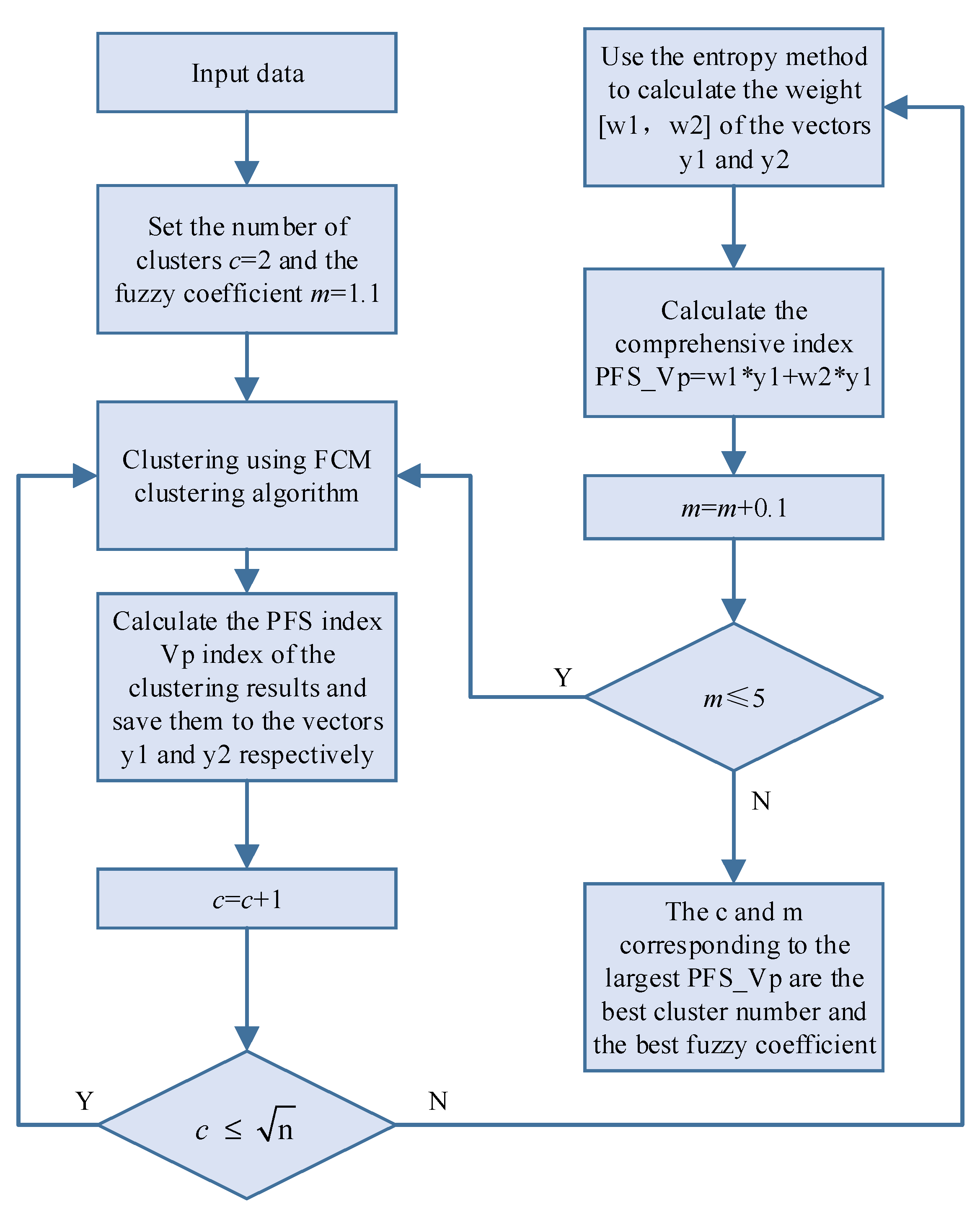
Figure 1. Improved FCM algorithm flow chart.
Processes 09 00907 g001
Figure 2. (a) Hourly data of temperature; (b) Hourly data of light intensity; (c) Hourly data of load.
Processes 09 00907 g002
Figure 3. (a) Separate clustering results of temperature data; (b) Separate clustering results of light intensity data; (c) Separate clustering results of load data.
Processes 09 00907 g003
Figure 4. (a) The maximum value of clustering index under different values of m; (b) the value of clustering index under different values of c when m takes the best value.
Processes 09 00907 g004
Figure 5. (a) PFS value under different values of c and m; (b) Vp value under different values of c and m.
Processes 09 00907 g005
Figure 6. The weight of the two indicators under different values of m.
Processes 09 00907 g006
Figure 7. PFS_Vp value under different values of c and m.
Processes 09 00907 g007
Figure 8. CCHP type microgrid structure diagram.
Processes 09 00907 g008
Figure 9. Flow chart of bi-level optimization configuration model.
Processes 09 00907 g009
Figure 10. (a) Heat load clustering result based on improved FCM algorithm; (b) Heat load clustering result based on improved FCM algorithm; (c) Electric load clustering result based on improved FCM algorithm; (d) Temperature data clustering result based on improved FCM algorithm; (e) Light intensity data clustering result based on improved FCM algorithm; (f). Probability of each clustering scene.
Processes 09 00907 g010
Figure 11. The relationship curve among fuzzy coefficient, cluster number, and comprehensive evaluation index.
Processes 09 00907 g011
Figure 12. (a) Pareto frontier; (b) comprehensive evaluation index of each solution.
Processes 09 00907 g012
Figure 13. (a) Single-level optimized Pareto solution set; and (b) best solution.
Processes 09 00907 g013
Figure 14. (a) Heat load clustering result based on FCM; (b) Heat load clustering result based on FCM; (c) Electric load clustering result based on FCM; (d) Temperature data clustering result based on FCM; (e) Light intensity data clustering result based on FCM; (f). Probability of each clustering scene.
Processes 09 00907 g014
Figure 15. (a) The pareto solution set FCM clustering result; (b) best solution.
Processes 09 00907 g015
Figure 16. (a) Daily operating cost and the total annual cost; (b) annual operating cost and the total annual cost.
Processes 09 00907 g016
Figure 17. (a) Daily carbon dioxide emissions; (b) annual carbon dioxide emissions.
Processes 09 00907 g017
Figure 18. (a) System operating costs in each scenario; (b) total operating cost of the system in all scenarios.
Processes 09 00907 g018
Figure 19. (a) System CO2 emissions in each scenario; (b) total carbon dioxide emissions of the system in all scenarios.
Processes 09 00907 g019
Table 1. Probability of clustering scene.
Scene NumberProbability of Temperature SceneProbability of Lighting SceneLoad Scenario Probability
17.95%4.38%12.05%
26.03%9.32%2.74%
311.78%5.48%4.93%
44.11%6.85%7.12%
53.56%7.67%18.08%
63.01%2.74%8.49%
76.03%5.21%8.49%
811.78%6.03%1.92%
94.38%9.86%6.85%
101.37%5.75%9.59%
114.38%5.21%3.84%
126.85%3.29%4.66%
131.64%8.77%3.56%
146.58%4.11%4.93%
154.38%8.49%1.64%
167.12%6.85%1.10%
173.56%————
185.48%————
Table 2. When m = 1.1, the values of PFS, Vp, PFS_Vp under different c values.
cPFSVpPFS_Vp
22.200036 9.25 × 10 8 0.784055
34.363254 1.65 × 10 7 1.554988
46.466143 8.44 × 10 8 2.304421
58.487213 7.48 × 10 8 3.024695
610.40768 4.06 × 10 8 3.709114
712.21195 4.42 × 10 8 4.352125
813.88793 4.27 × 10 8 4.949416
915.4271 3.03 × 10 8 5.497951
1016.82442 3.44 × 10 8 5.99593
1118.07806 3.52 × 10 8 6.442704
1219.18904 3.00 × 10 8 6.838638
1320.16081 2.92 × 10 8 7.184961
1420.99879 2.85 × 10 8 7.483601
1521.70987 2.76 × 10 8 7.737019
1622.30203 2.67 × 10 8 7.948056
1722.78393 2.35 × 10 8 8.119796
1823.16457 2.91 × 10 8 8.255449
1923.45302 2.68 × 10 8 8.358246
Table 3. The CCHP system energy station equipment parameter table of The Westin Xi’an Hotel.
ParameterValueParameterValueParameterValue
P mt 0 800 kW Q ec max 349 kW*3 + 180 kW*1 η es , chr & η es , dis 0.88
Q ac max 872 kW COP ec 5.54 & 5.6 τ hs 0.01
COP ac 1.2 Q gb max 2462 kW P hs , chr . max 150 kW
Q ex max 780 kW η gb 0.9 P hs , dis . max 200 kW
η ex 0.8 k op 0.067 ε hs max 0.95
P PVN 300 kW C gas 2.3 yuan / m 3 ε hs min 0
η es , chr & η es , dis 0.97 C mt 0.03 yuan/kWh C PV 0.08 yuan/kWh
τ es 0.02 C ac 0.025 yuan/kWh C es 0.02 yuan/kWh
P es , chr . max & P es , dis . max 100 kW C ec 0.01 yuan/kWh C hs 0.016 yuan/kWh
ε es max 0.9 C ex 0.025 yuan/kWh K co 2 , gas 0.23 kg / m 3
ε es min 0.2 C gb 0.02 yuan/kWh K co 2 , grid 0.972 kg/kWh
C grid 1.1098 yuan/kWh (7:00–11:00, 19:00–23:00);
0.7504 yuan/kWh (11:00–19:00);
0.3911 yuan/kWh (23:00–7:00)
Table 4. Pareto solution set.
No.PpvEesPesEhsf1f2No.PpvEesPesEhsf1f2
11021351783036,624,2417,255,373263101341104927,068,8707,002,639
21031201803076,627,5597,232,301273211341114867,081,1296,997,209
31011351792876,628,3797,256,557283351291154787,101,3636,964,088
41011421853056,628,9047,211,204293341271154787,111,4866,961,011
51021701613576,634,3807,230,568303331271154797,117,8426,991,920
61151641743526,697,8337,211,654313431321164827,120,3296,952,122
71261641753566,703,4877,200,944323511281084587,139,0126,947,780
81481621573326,721,2987,161,418333431431164947,143,9696,931,829
91591321413656,723,0927,145,922343531311134547,154,2766,928,483
101501331553646,724,7577,156,029353571381104477,159,4086,924,401
111601331553646,753,3467,134,707363751141094527,173,2816,919,122
121561321453656,754,4487,141,065373671401014327,175,4836,915,743
131813341021996,832,9677,114,179383741361094467,176,3996,906,823
141863251051946,834,5447,118,199393721361094467,187,4866,901,102
151893251061936,842,7767,101,519403831541004727,201,5046,895,461
161943241021986,866,7947,101,474413831551004737,206,5176,895,513
172013301031956,883,2237,098,761423911191044487,213,1836,874,998
182133311032056,883,8637,095,332433921701054497,252,0476,879,032
192043061522346,885,2537,110,427444041681074527,254,6936,874,154
202143251062126,887,5307,067,371454041631144337,261,4296,871,308
212093371141886,895,6767,089,063464051631074537,269,0186,841,216
222133301062116,902,7677,074,296474151711084587,287,0066,865,981
232243651001896,926,2457,049,328484241851084607,339,2516,852,201
242293321051876,933,2347,044,454494645531584867,516,5276,844,550
252393331212486,965,5397,047,380504645481604887,569,9346,837,387
Publisher’s Note: MDPI stays neutral with regard to jurisdictional claims in published maps and institutional affiliations.