2.3. Implementation of the DDQL Algorithm for Pass Schedule Design in Open-Die Forging
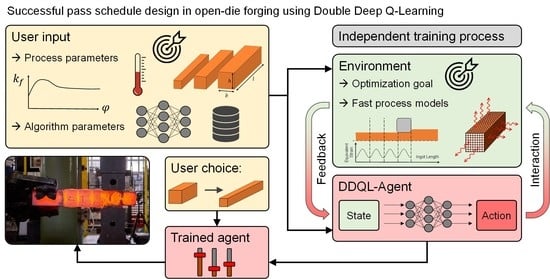
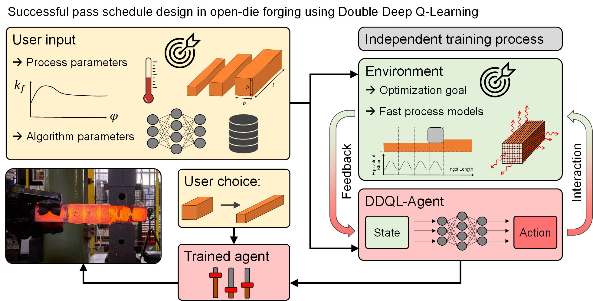
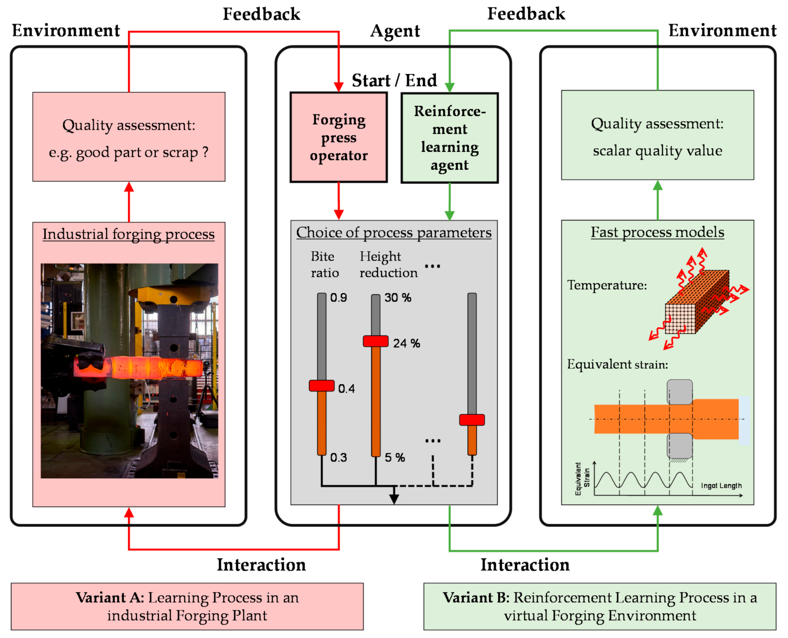
Here, a reinforcement learning DDQL algorithm is presented that is supposed to generate optimized pass schedules following defined goals. The DDQL algorithm was chosen since deep Q- and double deep Q-learning are used successfully to solve various engineering problems [
39,
40,
41] including the optimization of the production of multilayered optical thin films [
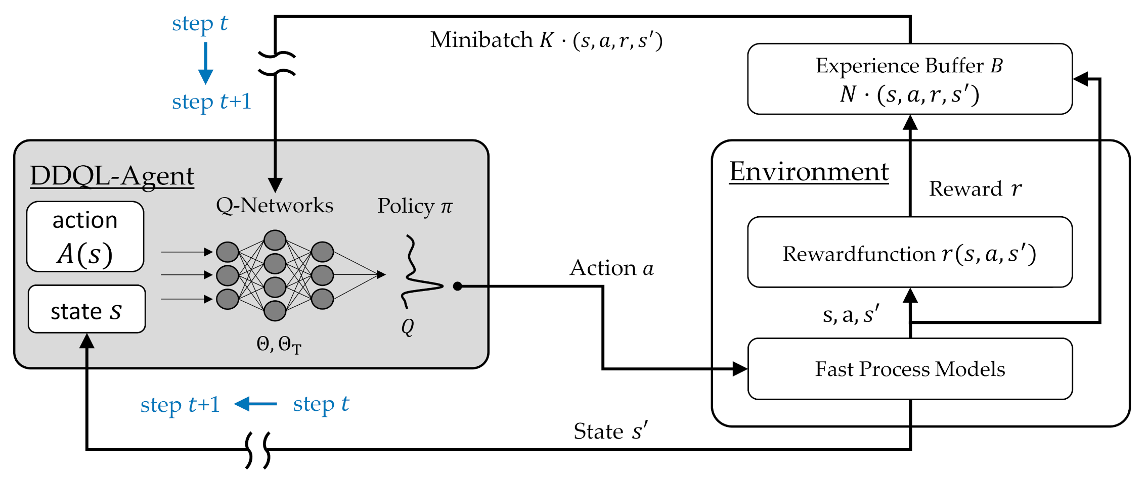
42] whereby, as in the optimization of open-die forging processes, different highly nonlinear physical relations need to be considered. The developed algorithm was implemented in MathWorks MATLAB and consists, as described in
Section 2.2 and shown in
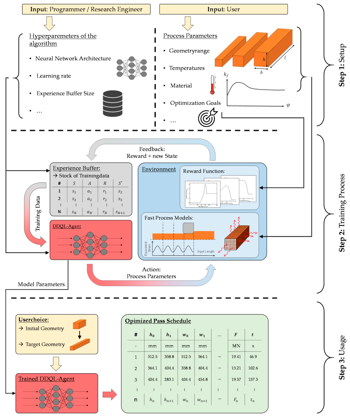
Figure 4, of two main elements interacting with each other: The agent and the environment.
The state
of the environment represents the current state of the forging block and is characterized by five normalized values: The ingot height,
, at the start of the current state,
, the difference,
, between the target height,
, and the current height,
, the mean equivalent strain in the core fiber,
, the mean temperature in the core fiber,
and the mean surface temperature,
. These values were chosen based on their process information content. The current ingot height,
, and the height difference,
, carry needed information about the current and the target geometry and, hence, enable an estimation of the remaining process length. Since the press force is used as an optimization criterion (cf.
Section 2.6), the temperature (
,
.) and equivalent strain (
) information are required, allowing a prediction of the current yield stress and consequently a prediction of forces. In addition, the mean surface temperature and the mean core temperature result in a gradient that usually increases over the course of the forging process and, consequently, allows in combination with the current ingot height,
, a rough estimate of the previous process duration and the current temperature field. Based on this state information,
, the agent selects the next action,
, which consists of the two process parameters: bite ratio,
and height reduction,
. In contrast to the state information,
, which consists of continuous values, the action selection of the agent is limited to discrete steps. In the present algorithm, the bite ratio,
, can be varied between 0.3 and 0.9 in steps of 0.05 and the height reduction between 3% and 30% in steps of 1%.
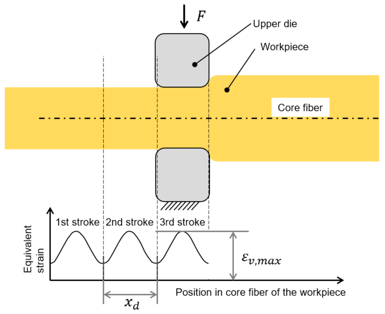
To ensure the accuracy of the calculations from consecutive state transitions within a pass schedule, the spatially resolved information about the temperature and the equivalent strain distribution along the core fiber was stored within the environment. In subsequent passes, this information was used as the point of departure of the state transition calculations using the fast process models. Afterwards, the above-described averaged values were determined and merged together with the current geometry information in the form of the five tuple representing the resulting state .
In addition to the process parameters, such as the current ingot height or the selected height reduction , which can be directly related to the open-die forging process, the algorithm also contained parameters without a direct physical background or reference to the forging process. These included, for example, the model parameters and of the Q-networks, which were first learned during the training process using experience data tuples . Since these learned model parameters cannot be physically interpreted on their own but significantly determine the behavior of the later used algorithm and, thus, the quality of the designed pass schedules, only an indirect connection between model parameters and the forging process was present. On the other hand, the algorithm has so-called hyperparameters that are not learned during training but are predefined by the user and have no direct connection to the forging process either. Since hyperparameters significantly determine the training process of the algorithm, there is nevertheless an influence on the quality of the generated pass schedules, for example, through improved convergence properties or higher average rewards.
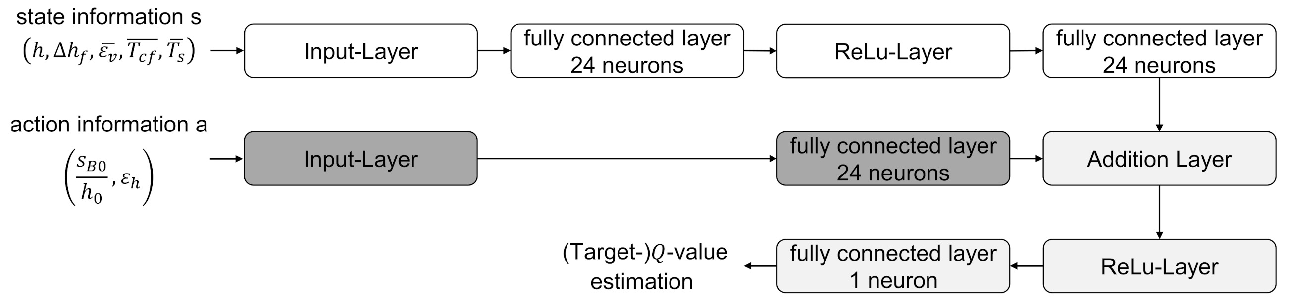
To approximate the Q- and target Q-values, the agent used a neural network that had two separate input branches: one for state information and one for action information. The action information was normalized and fed into the neural network by an input layer. This was followed by a fully connected layer with 24 neurons and a subsequent addition layer. This addition layer combined the pre-processed information from the two branches by an element-wise addition. In the state branch, the normalized information was also fed into the net via an input layer. Two fully connected layers followed, which were separated by a ReLu layer. The abbreviation ReLu stands for “rectified linear unit” and corresponds to the mathematical operation
, where negative values are set to zero and non-negative values remain unchanged. The output of the second fully connected layer was connected to the addition layer, followed by another ReLu layer. Finally, a fully connected layer with a single neuron formed the output layer which had a value that corresponded to the estimated Q- or target Q-value. The used network architecture was proposed in [
43] and shown in
Figure 5.
To ensure the algorithm not only relies on its experience during the training process but also sufficiently explores the state space
and action space
, an ε-greedy-policy was used to maximize the return,
, obtained in the long run [
31]. Here, a random action,
, was chosen with the probability
and, otherwise with the probability of
, a greedy action with respect to the
value according to Equation (10) was selected. For this purpose, the agent needed to calculate the
values of each combination of the current state
and all possible actions
separately. This was necessary because the implemented
-network architecture (cf.
Figure 5) uses not only the state information
but also action information
to determine the
value of a single state–action pair. The probability ε for a random action choice does not remain constant over the training process. Starting from a value of 1,
decreases continuously in every training time step
according to the selected epsilon decay rate of 0.0001 to a minimum value
(cf. Equation (15)). These hyperparameters are based on literature values [
35] that were adapted to the conditions of the DDQL implementation in MathWorks MATLAB.
With the selected action
and the present state
the environment was able to calculate the change of state of the forging block
using the fast process models presented in
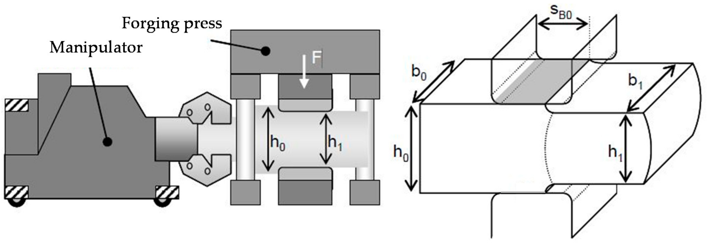
Section 2.1. A change of state does not correspond to just one pass, but always to two passes, where the forging block is rotated by 90° around the longitudinal axis after each pass. For this purpose, the bite ratio
selected by the agent was used in both passes, while the selected height reduction
was only used in the first pass. The height reduction in the second pass was determined in such a way that after the pass a square billet cross-section
was created, taking the occurring width spread into account (see Equation (1)). This forging strategy with a square ingot cross-section after every second pass is called “square forging” and is widely used in industrial applications. Subsequently, fast process models were used to calculate the development of the temperature field and the equivalent strain distribution during both passes (see
Section 2.1). Finally, the values of the state information s’
were put together and transferred to the reward function and the training data memory
as shown in
Figure 4.
The hyperparameters experience buffer size
data sets, and the size of the mini-batch
= 64 randomly chosen data sets was taken from the default settings of the DDQL implementation in MathWorks MATLAB [
44]. As described in
Section 2.2, the mini-batch was used to adjust the parameters
and
of the Q- and Target Q-networks. The learning rate
determines the size of the individual adaptions and had to be lowered from the default value
to
based on some test trainings that showed unstable training behavior and convergence problems.
The reward function,
(cf.
Figure 4), is the part of the implementation in which the user defines the goals of the algorithm during the training process. For this purpose, a mathematical formulation
must be found that represents the goals in such a way that the algorithm achieves them by maximizing the received return
. Hence, the reward
corresponds to the quality of an action choice consisting of the bite ratio and height reduction within a defined ingot state
, considering the defined optimization goals.
The goals for the present application example of a pass schedule design in open-die forging were aligned to the possibilities offered by comparable pass schedule calculation software without methods of artificial intelligence (see
Section 1). The first goal a pass schedule should fulfill is to reach the target geometry, whereby a permissible percentage deviation,
, is tolerated. Here, this permissible deviation is one percent and is thus within the usual range for open-die forging [
45]. Two further criteria for an optimal pass schedule design are derived from the desire to make the process as fast and efficient as possible. On the one hand, the final geometry should be achieved in as few passes as possible and, on the other hand, the available machine force,
, should be used in the best possible way. For this purpose, the desired target force,
, was set at 80% of the maximum press force,
, to consider a sufficient safety margin.
Through this selection of optimization criteria with a force and a pass number component, the complicated incremental process kinematics and geometry development in open-die forgings were taken into account. If only the press force is evaluated, the algorithm could tend to apply the largest possible bite ratios while using small height reductions, resulting in long forging processes. This effect is intensified by the occurring width spread, since width spread increases with increasing bite ratios and must be forged back in the subsequent pass due to the 90° ingot rotation at the end of each pass.
On the other hand, the pure evaluation of the number of passes can lead to an algorithm selecting the largest possible height reductions combined with small bite ratios, as in this case little width spread occurs and, overall, the fewest passes are required. However, such a forging strategy can cause surface defects in the billet, such as laps, and is therefore not desirable. In addition, small bite ratios result in high numbers of strokes, which increase the process time.
Moreover, the sole evaluation of the process time is not implemented, because the process time is highly individual for each plant, as it strongly depends on the present velocities and accelerations of the manipulator and of the forging press. In addition, discrete events, such as a significant increase in time due to reheating, can hardly be weighted reasonably within the complex process optimization framework.
In Equations (16)–(18), the complete mathematical formulation of the used reward function
is summarized. The function is divided into two large subareas, the evaluation of the geometry and the evaluation of the occurring maximum press force:
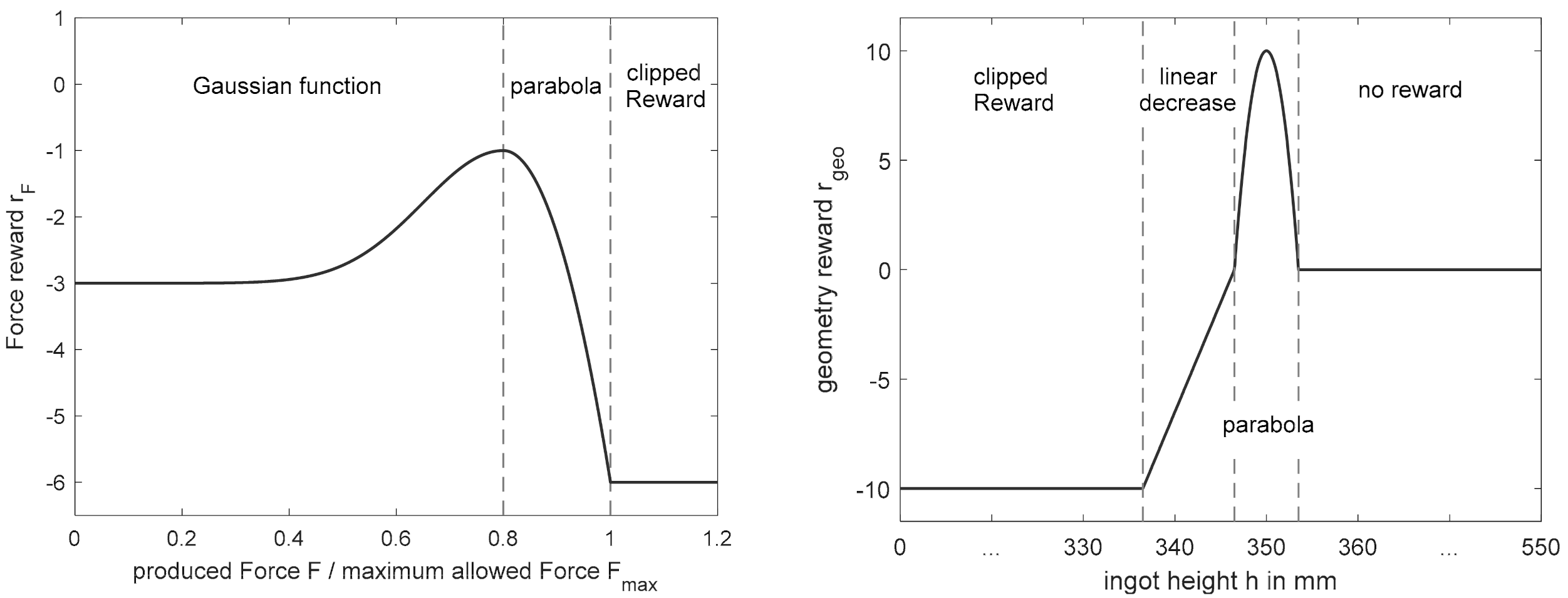
The reward for the generated geometry,
(see Equation (17)), evaluates only the final generated ingot height of a pass schedule and not the intermediate geometry development during the forging process, as the continuous evaluation of the ingot height could cause contradictions with the other optimization goals. If the permissible final height range,
, is met, the reward according to Equation (17) corresponds to a symmetrical parabola that reaches its maximum of 10 at
and has the value 0 at the edges. If the algorithm generates a final height,
, that falls below the minimum permissible height,
, the reward corresponds to the resulting difference,
. The resulting overall function for the evaluation of the block geometry,
, is shown in
Figure 6 (right) showing an example target height,
.
Equation (17) also shows that the penalty for dropping below the final height has a lower limit of –10. This procedure is derived from the reward clipping recommended in [
36] and can significantly improve the convergence properties of an algorithm, since individual rewards with high values can lead to large adjustments in the Q-function and, thus, to instability in the training process.
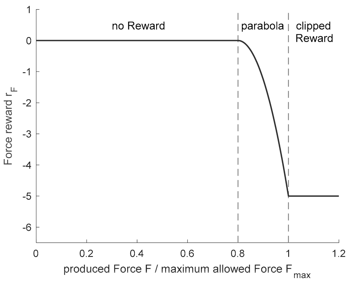
The evaluation of the maximum force,
, occurring in the two passes of the state transition
was divided into different scenarios according to its value and according to the block height,
, in state
(cf. Equation (18)). As long as the generated height
is above the allowed end range
, the reward
is calculated as shown in
Figure 6 (left) either by a Gaussian function or a parabola, depending on the calculated force,
. If the resulting force,
, corresponds exactly to the target force,
, the reward
reaches its maximum. If the force decreases starting from the maximum
, the reward drops to −3, while for forces above
, rewards up to −6 are possible. This asymmetry is due to the fact that exceeding the target force is more critical than undercutting it. If the force,
, rises above the maximum press force,
, reward clipping comes into effect again and limits the reward,
, to a minimum of −6.
If a block height is generated that is in the range of the permitted final heights or below, the completed change of state describes the last two passes of a pass schedule. In these passes, the focus is primarily on setting the desired final geometry and not on the optimal use of the press force, which is why the force reward for forces below the target force,
, is omitted (cf. Equation (18) and
Figure A1 (
Appendix A)). However, since the maximum press force,
, must be maintained in the last two passes as well, the rest of the force evaluation (
) remains qualitatively unchanged.
The reward for the generated forces, , is not arbitrarily defined negatively, but it represents the goal of using the smallest possible number of passes. This results from the fact that the algorithm tries to maximize the received return, , in the course of the training and, consequently, shows a tendency to lower the number of passes, because at lower numbers of passes negative force rewards are received less often.
The total reward of an action choice is finally calculated according to Equation (16) from the sum of the geometry reward, , and the force reward, . The total reward of an action choice is also limited by reward clipping to a minimum value of −10. Therefore, the clipped sum of the individual rewards is always in the range [−10, 10] and can be scaled to the required order of [−1, 1] using the divisor 10. The general weighting of the individual parts of the reward function arose from the prioritization of the defined goals. Therefore, the reward for reaching the final geometry was set proportionally higher than the cumulative punishment of the force utilization, respectively, the number of passes. The exact weightings were determined by many test trainings.
In summary, the general characteristic of the reward function is that the focus in each of the last passes of a pass schedule is primarily on reaching the desired final height as accurately as possible and in all preceding passes, mainly on making the best possible use of the press force. To emphasize this characteristic, the discount factor
was reduced from the default value
= 0.99 to 0.9. Since the geometry reward is achieved only at the end of each training pass schedule, it tends to be discounted more often by the discount factor. As a result, the influence of the geometric reward granted for hitting the target height decreases in preceding passes and using the press force optimally becomes more important. However, the discount factor must not be selected too low either, since in a state
, the algorithm can only select discrete actions,
, and, thus, the resulting block heights,
, are also limited. In addition, the permissible deviation from the target height,
=
, is small, and the reward received rapidly decreases with increasing distance from the optimal value
, even within the permissible deviations (see
Figure 6 (right)). Consequently, it may be necessary for the algorithm to adapt its actions over several passes in advance in such a way that the target height is hit as accurately as possible, thereby maximizing the total reward.
2.6. Evaluation of the Algorithm Performance
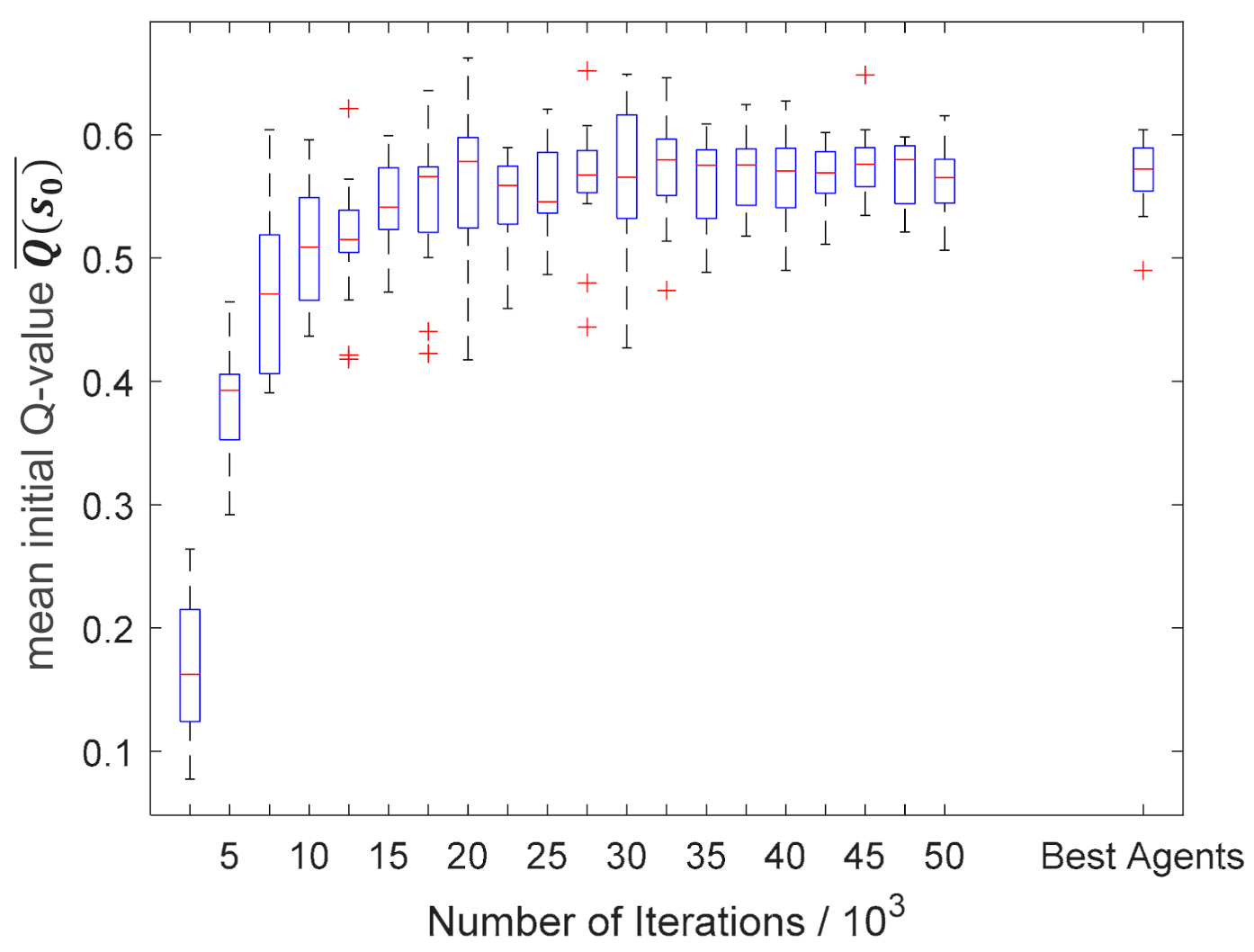
To evaluate the performance and the convergence of a reinforcing learning (DDQL) algorithm, commonly the generated rewards or the Q-value of the initial state,
, are plotted over the iterations of the training process [
31,
35,
36,
37,
38]. If the training is successful, both values increase during the training and, in the best case, converge towards their optimum.
If an algorithm performs well measured by the generated total reward or Q-values, it is only a reliable indicator for the achievement of the defined training goals as long as the reward function is a sufficiently accurate mathematical representation of these goals. Although this condition is assumed in the present implementation, it must be checked nevertheless in the analysis of the training results. Therefore, the performance and the convergence of the algorithm are measured not only by the collected total rewards of individual iterations or the -value, but additionally by the development of the following process parameters and auxiliary variables, which directly represent the defined goals:
Difference between the generated final height and target height ;
- ○
Goal: accurately achieve the desired final height ;
Number of passes ;
- ○
Goal: minimize the number of passes;
Maximum force occurring in the pass schedule ;
- ○
Goal: stay below the press force limit;
Force utilization
- ○
Goal: best possible utilization of the forging press.
The force utilization,
, corresponds to the sum of the absolute differences between the maximum generated force,
, and the target force,
, over all state changes that make up the evaluated pass schedule (see Equation (19)). Since the force of the last pass is not evaluated in the training process, it is also dismissed from the force utilization calculation. This procedure is based on the fact that the forces of the two passes, which are derived from the selection of an action
, were not selected independently of each other due to the square forging.
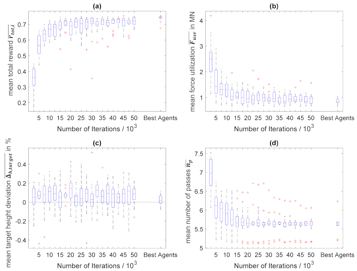
Furthermore, due to the underlying non-continuous problem of pass schedule design in open-die forging, only short training iterations with mostly single-digit training step numbers occur in the present algorithm. At the same time, the structure of the reward function leads to the fact that the negative force reward is received less frequently with lower numbers of passes, which means not every combination of initial and target height can achieve the same maximum total reward. Since the start and target heights of a pass schedule are chosen randomly in the training process, the maximum possible reward is not constant within individual training iterations. For this reason, the convergence and performance of the algorithm is not measured by the characteristics of pass schedules of individual combinations of initial and target heights, but by parameters averaged over the entirety of input parameters.
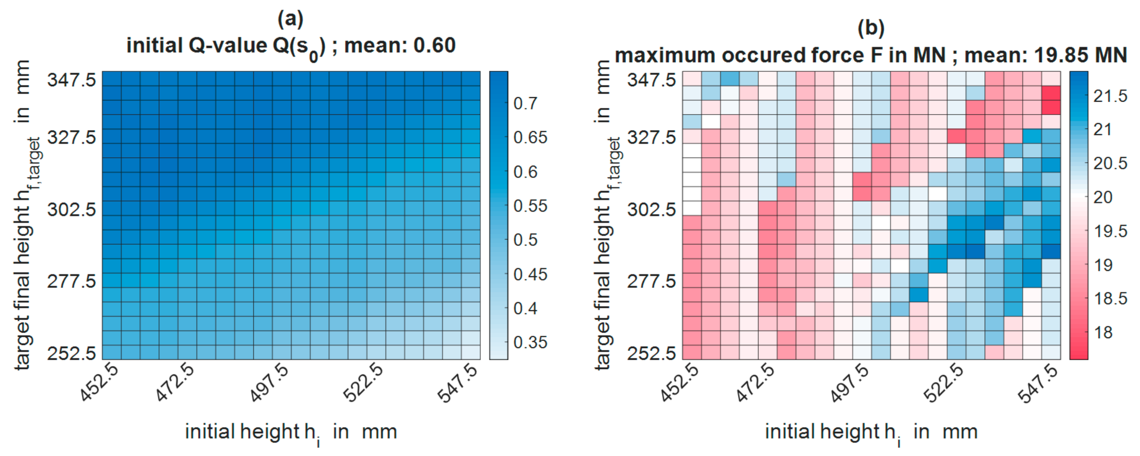
To generate these mean values for different training states, the algorithm was evaluated every 2500 training iterations. The input parameters initial and target height were both varied in 20 steps, resulting in 400 evenly distributed parameter combinations. With the help of the current agent, a pass schedule was designed for each of these combinations and the abovementioned characteristic process and algorithm parameters were stored. Subsequently, an average value can be calculated for each characteristic variable across all 400 pass schedules of an evaluation step. The pass schedule design using a fully trained algorithm works in the same way as the pass schedule design during the training process, with the difference that instead of the ε greedy policy, a pure greedy policy according to Equation (10) is used.
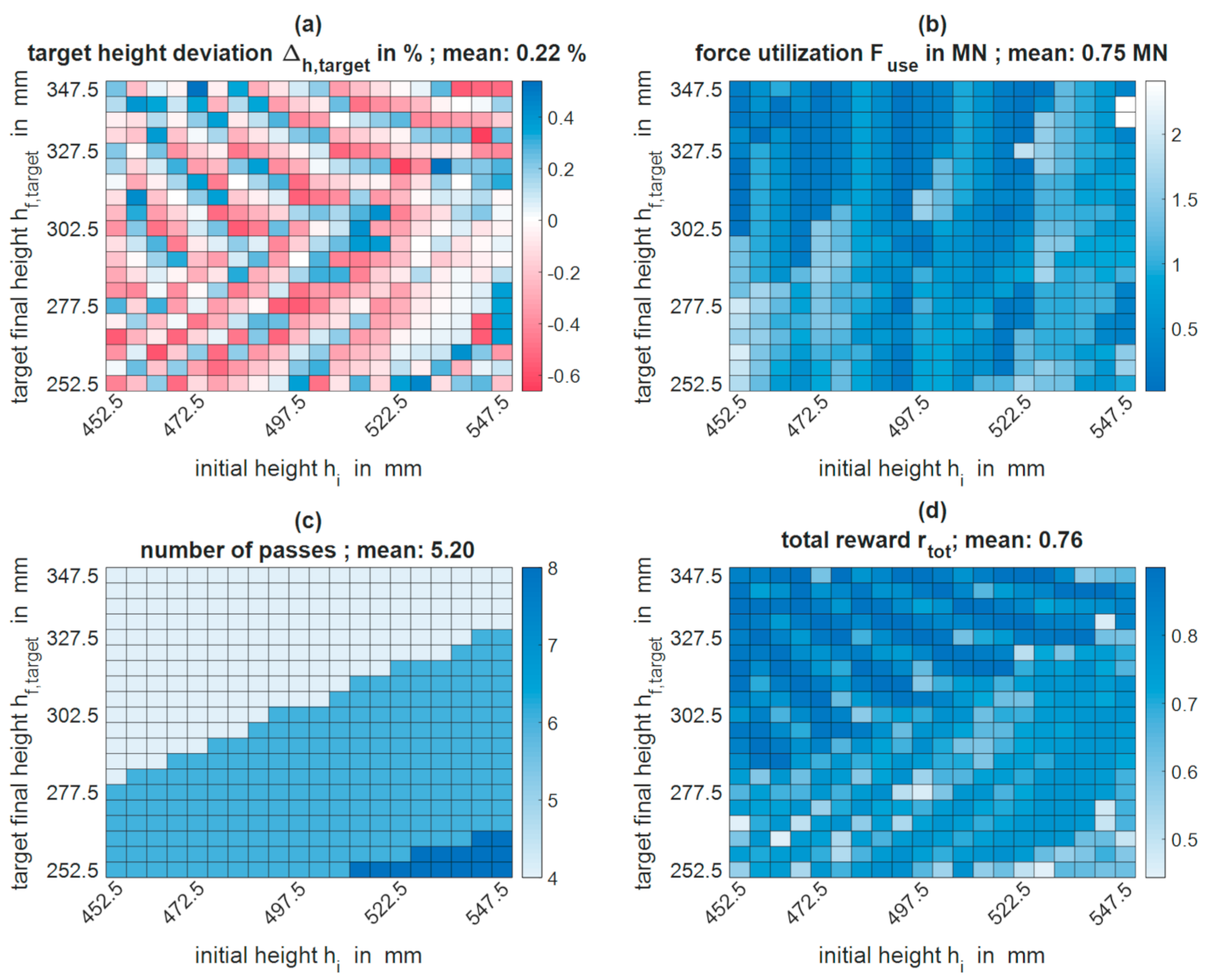
Machine learning algorithms and especially neural networks represent black boxes which have a learning process and behavior that is very difficult or even impossible to comprehend. Therefore, the characteristics of the evaluated pass schedules are graphically refurbished to provide an insight into the behavior and the learning process of the algorithm. For this purpose, the respective characteristic parameter was plotted over the varied initial and target heights, and the individual areas were colored according to the value of the characteristic parameter. So-called heatmaps (cf.
Section 3.2) arose, which enable the user to utilize his process knowledge of open-die forging to analyze the behavior of the algorithm more precisely. For example, the user can examine which training goal is already achieved for which combinations of initial and target heights or the user can analyze which process and algorithm parameters correlate.
Exactly the same algorithm might converge in one training delivering good results and diverge in another seemingly identical training producing no useful training results. This is related to random influences on the training process such as the initialization of the (target) -network and the epsilon-greedy policy. In order to ensure that the convergence of the algorithm and the generated training results are not purely by chance but resilient, the training process was carried out and analyzed 15 times with the same algorithm and process parameters but different random seeds over 50,000 training iterations each.
The training processes lasted approximately two days performed on an Intel CPU of type Xeon E-2286G. This training duration results primarily from the calculation of the environment and not from the adjustment of the network parameters. Since the DDQL algorithm has an experience data memory and consequently learns “off-policy”, the generation of experience data sets can be parallelized in the future, so that the training duration may be reduced significantly.


