Abstract
The integration of solar energy in smart grids and other utilities is continuously increasing due to its economic and environmental benefits. However, the uncertainty of available solar energy creates challenges regarding the stability of the generated power the supply-demand balance’s consistency. An accurate global solar radiation (GSR) prediction model can ensure overall system reliability and power generation scheduling. This article describes a nonlinear hybrid model based on Long Short-Term Memory (LSTM) models and the Genetic Programming technique for short-term prediction of global solar radiation. The LSTMs are Recurrent Neural Network (RNN) models that are successfully used to predict time-series data. We use these models as base predictors of GSR using weather and solar radiation (SR) data. Genetic programming (GP) is an evolutionary heuristic computing technique that enables automatic search for complex solution formulas. We use the GP in a post-processing stage to combine the LSTM models’ outputs to find the best prediction of the GSR. We have examined two versions of the GP in the proposed model: a standard version and a boosted version that incorporates a local search technique. We have shown an improvement in terms of performance provided by the proposed hybrid model. We have compared its performance to stacking techniques based on machine learning for combination. The results show that the suggested method provides significant improvement in terms of performance and consistency.
1. Introduction
With the increased interest in energy preservation and environmental protection, the world today is moving into a transition from almost total dependence on fossil fuel to the increased use of alternative sources of energy. Solar radiation (SR) is one of the promising and potential renewable energy sources [1,2]. Short-term forecasting of SR plays a significant role in assessing the feasibility of actual applications in smart balanced grids between power production and consumption at a given interval of time [1,2,3,4,5]. Therefore, it plays an essential role in several aspects of smart grids scheduling management and renewable energy engineering. This fact requires reliable techniques to predict the stochastic dependency between present and future values of SR using available observations.
Machine learning techniques have gained attention as good competitors to classical statistical models in prediction [5,6,7,8,9]. Machine learning models are considered as nonlinear data-driven models. They use prior data records to recognize the stochastic dependency between past and future data sequences.
Many machine learning models have been suggested to forecast the global solar radiation (GSR), namely Artificial Neural Networks (ANN), Support Vector Machines (SVM), Random Forests (RF), Decision Trees (DT), and Regression Trees (RT) [9,10,11,12,13,14].
In general, consistency and stability are the main challenges researchers encounter in designing consistent SR forecasting models. It is particularly true when dealing with stochastic time-series data.
Ensemble learning techniques that consist of aggregating the decisions of several individual models, also named weak learners, have been proposed for forecasting. In general, the main idea behind the ensemble technique is to combine the outcomes of multiple learners that could be complementary to each other, since it is unlikely that all predictors make the same prediction faults. The stacking ensemble technique is one of the contemporary ensemble techniques; it uses a machine learning model, also named the meta-model, to aggregate the decisions of the weak learners of an ensemble [4,7].
Lately, several machine learning ensemble techniques have been proposed to enhance the short-term prediction of SR power, SR energy strength, and wind energy [15,16,17,18,19,20,21,22,23]. Table 1 summarizes some ensemble models in the literature that have been proposed for the prediction of SR and wind energy along with their base learners and ensemble types.

Table 1.
Summary of reviewed ensembles and combinations for SR energy forecasting.
All the above-mentioned ensemble methods are either based on probabilistic combination, weighed sums, or stacking techniques. It is worth noting the stacking techniques. Even though they provide smart combinations of base learners instead of just applying a simple averaging of outputs, they still have some limitations. The main limitation of those techniques is finding the optimal structure and parameters of the machine learning models that are designed for stacking. This limitation becomes obvious when the training dataset dedicated to train the meta-model is small and insufficient to train that model (under-fitting problem).
In this research, we suggest a framework that consists of a meta-heuristic optimization method, named Genetic Programming (GP), that aims to find the optimal combination of the outputs of individual predicators, also called weak learners, of an ensemble. The GP optimization is inspired by the natural selection of individuals that represent solution candidates, based on a fitness objective function. The fittest individuals with high fitness functions are selected to survive for the next generations through a competitive evolutionary computation [24,25,26]. The individuals in our case are the formulas of the combination of the base predictors’ outputs. The GP module aims to find the best combination of formulas that minimizes the overall prediction error of the committee of base learners. Our experiments examined two versions of GP, a standard version and a hybrid one named Memetic Programming (MP), boosted by a local search technique [27,28]. The incorporated local search technique permits increasing the exploitation of the GP module when searching for the optimal solution.
In solar energy estimation and SR prediction literature, the GP and other heuristic computation techniques have been used directly on collected weather and solar measured data to estimate or predict the SR strength [29,30,31,32,33,34,35].
In [29], the authors utilized Linear Genetic Programming (LGP) to predict the GSR using weather data. The GSR is formulated in terms of climatological and meteorological parameters in two specific areas of Iran. The authors elaborated and validated two separate models for each of the two regions, and they evaluated the significance of each parameter of the dataset by applying a sensitivity analysis. The authors claimed that the performance of their LGP-based models outperforms those based on angstrom’s models. In [30], the authors applied the GP technique to estimate the reference evapotranspiration in California—USA using daily atmospheric parameters such as the daily mean temperature, daily SR, average daily humidity, etc. The comparative experiments of the authors show that their proposed GP-based model outperformed the performance of other conventional models such as the Penman–Monteith equation, the Hargreaves–Samani equation, the Jensen–Haise equation, the Jones–Ritchie equation, and others. In [31], the authors proposed a Multi-Gene Genetic Programming (MGGP) model to estimate SR in Turkey. The model accepts as inputs some meteorological data such as extraterrestrial SR, sunshine duration, mean of monthly maximum sunny hours, long-term mean of monthly maximum air temperatures, and other parameters. The authors concluded that the MGGP model results for SR prediction were more accurate than the values achieved by some conventional empirical equations such as Angstrom and Hargreaves–Samani. The performance of MGGP is also assessed by single-data and multi-data models. The multi-data models of MGGP and calibrated empirical equations are more performant than the single-data models for SR estimation. In [32], the researchers employed the GP techniques on climatological data to elaborate the best function predicting the solar panel’s temperature (Tpanel) for a product family of polycrystalline solar panels. The data recorded include SR measurements with ambient temperature, wind velocity, and ambient relative humidity as effective parameters. The authors claimed that their obtained function outperformed the models related to the Nominal Operating Cell Temperature (NOCT) and Nominal Module Operating Temperature (NMOT) approaches that are considered as the most common ways to obtain the Tpanel. In [33], the authors presented a hybrid approach that includes the GP and the Simulated Annealing (SA) heuristic optimization techniques for estimating the GSR. The researchers concluded a prediction equation where the SR is formulated in terms of several climatological and meteorological parameters in two cities of Iran.
In [34], the authors investigated the capacity of neural networks models and the Gene Expression Programming (GEP) technique for estimating daily dew point temperature by using daily recorded data that include incoming SR, atmospheric pressure, dew point temperature, and other parameters. The researchers concluded that the GEP models outperform the ANN models in estimating daily dew point temperature values. In [35], the authors proposed a nonlinear regression model based on GP techniques for estimating SR. The best nonlinear modeling function obtained takes into account the measured meteorological data. An enhanced approach that consists of multi nonlinear functions of regression in a parallel structure is presented. Each function is designed to estimate the GSR in a specific seasonal period of the year.
The above-described methods and most of the reported approaches in the literature that use the GP-based techniques for predicting SR and other types of energies apply the GP directly in the weather parameters. In this research, we propose a hybrid framework that uses the GP on finding the optimal combination formula of the outputs of time-series data predictors of the Long-Short term Memory (LSTM) type. We believe that applying the GP or any other heuristic optimization technique directly on weather and solar data will not cope (handle) with this data type [32,33,35]. The proposed hybrid framework employs the GP in a post-processing phase to combine outputs of base recurrent predictors of type LSTM [36,37]. The LSTM is a gated machine learning model that is trained using the gradient-based Back-Propagation Through Time (BPTT) algorithm. The BPTT is a new version of the classical back-propagation gradient descent algorithm suitable for recurrent models. Nowadays, the LSTM models are considered one of the most prominent Recurrent Neural Networks (RNN) models for deep learning to solve time-series data forecasting problems. They are suitable for modeling and handling time-series data frames by handling the temporal context among serial data records. The proposed method combines the superiority of LSTM models to model time-series data with the capacity of heuristic models to explore the best nonlinear combination formulas. The base forecasters and the heuristic combination module were designed for the short-term prediction of SR intensity.
The main contribution of this research is to propose a hybrid LSTM-based GP approach for the short-term prediction of GSR. The approach consists of an ensemble of homogeneous base models of the LSTM type combined by a weighted formula designed by a heuristic optimization technique of the GP type. This work also validates and compares the performance of two versions of the GP technique for our approach in terms of performance and consistency. In all the hybrid models considered in this research, the examined predictors aim to predict the amount of GSR in a horizon fifteen minutes ahead using the measured amount of GSR and weather data for the previous n slots of 15 min. Moreover, the proposed approach has been compared against machine learning based stacking techniques. The performance of the considered models has been evaluated using statistical metrics and graphical methods. The rest of the paper is organized as follows: Section 2 introduces the GP and LSTM, and it presents the GP versions and frameworks that we used in our experiments. Section 4 illustrates the structure and the implementation of the proposed method. In Section 5, we present and discuss the experimental results and their interpretation. Finally, the paper is concluded in Section 5.
2. Genetic Programming and Long Short-Term Memory Models
2.1. Genetic Programming
GP is an extension of the conventional Genetic Algorithm (GA), which is inspired by the biological processes of natural selection and survival of the fittest [24,38]. The main difference between GA and GP lies in representing a solution, where GA usually uses an array of bits to represent a solution. In contrast, GP deals with functions (computer programs) represented as tree data structures [24,25,26]. Each tree in GP comprises sets of nodes, where internal nodes represent algebraic and/or logical operators. In contrast, the external ones, called terminals, represent the numbers and data variables of the given problem. Figure 1 depicts examples of binary trees representing mathematical functions, where each function can be seen as a computer program.
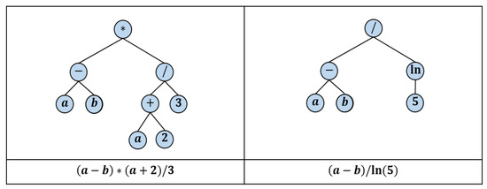
Figure 1.
Examples of trees that represent algebraic functions.
The GP algorithm uses the so-called genetic operators—crossover, mutation, and cloning (reproduction)—to generate a new population from the current one. This process is repeated until it reaches an optimal solution or reaches the maximum number of iterations [38]. The algorithm starts with an initial population of trees, also named individuals, that are usually generated randomly. Then, in each generation of individuals, the GP algorithm performs the following steps:
- Measure the fitness value for each individual using a predefined fitness function. This fitness value indicates how the individual function (computer program) suits the problem under consideration.
- Select a set of individuals, based on their fitness values, from the present population using a suitable selection strategy.
- Generate the next population by applying the crossover and mutation operators to selected individuals based on predefined crossover and mutation probabilities.
- Based on a predefined reproduction probability, the clone is based on individuals with the best fitness values to the next population.
These steps are repeated until an optimum solution is found or the maximum number of fitness evaluations is reached. Figure 2 illustrates an example of applying the crossover operator on two selected individuals.
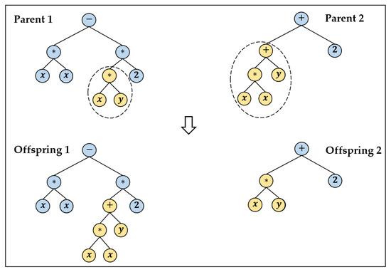
Figure 2.
The crossover of two individuals to produce two new ones (Offsprings) for the next generation.
Several selection strategies for the GP algorithm are introduced and studied extensively, all of which make use of the fitness values of the current population. In this paper, the tournament selection, of size is used, where individuals from the current population are chosen randomly, and the one with the best fitness is considered as the winner. Moreover, the fitness value of an individual is calculated as the Root Mean Square Error (RMSE) as follows:
where is the predicted output and is the measured value related to that output.
In the following sections, two modified versions of the GP algorithm are introduced.
2.1.1. GPLearn Framework
The GPLearn framework implements GP in Python language with compatible API [39]. GPlearn includes all the standard features to design and validate a GP optimization model. Plus, it provides three alternatives of mutation operation, namely the sub-tree mutation, the hoist mutation, and the point mutation. Those operators permit increasing the exploration capability of the GP implemented in this framework. They operate as follows:
- Sub-tree mutation: it takes the winner (a tree) of a random selection and then selects a random sub-tree from it to be replaced. A donor sub-tree is generated at random, and this is inserted into the chosen winner tree to form offspring in the next generation. This type of mutation is considered one of the aggressive mutations. It allows big changes in an individual by replacing a complete sub-tree and all its descendants with totally naïve random components.
- Hoist mutation: it takes the winner of a random selection and selects a random sub-tree from it. Then, a random sub-tree of that sub-tree is selected, and this is lifted (hoisted) into the original sub-tree’s location to produce offspring in the next generation.
- Point mutation: it takes the winner of a random selection and selects random nodes from the winner to be replaced. Functions are replaced by other functions that require the same number of arguments, and other terminals replace terminals. The resulting tree forms offspring in the next generation. Figure 3 depicts the three described types of mutations.
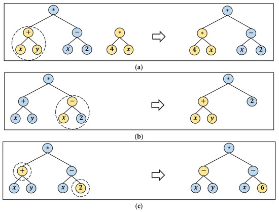 Figure 3. Advanced mutation operators implemented in GPLearn. (a) Sub-tree mutation, (b) Hoist mutation, and (c) Point mutation.
The GPLearn framework is purposefully constrained to solve symbolic regression problems. Symbolic regression is a machine learning technique that aims to identify an underlying mathematical expression that best describes a relationship among dependent and independent variables. It begins by building a population of simple random formulas to represent a relationship between known independent variables and their dependent variable targets to predict new data. Each successive generation of programs is evolved from the one that came before it by selecting the fittest individuals from the population to undergo genetic operations. GPLearn supports regression through the SymbolicRegressor class and binary classification with the SymbolicClassifier Class. This open-source framework evolved through many versions. The latest version is 0.4.1 through which we have built our GP model.
2.1.2. Memetic Programming
The Memetic Programming (MP) algorithm is a hybrid evolutionary algorithm that searches for suitable functions (computer programs) for a given problem. Each loop of the MP algorithm contains two different types of searches: diversification search and intensification search. The MP algorithm uses the GP operators, crossover and mutation, to guarantee the diversity in the current population. Then, the algorithm employs a set of local search procedures to intensify the best individual programs of the current population. Specifically, these local search procedures generate new trees from a given tree by using shaking, grafting, and/or pruning operators [27,28]. The shaking operator generates a new tree from by altering its nodes without changing its structure. On the other hand, grafting or pruning operators change the structure of by expanding its terminal nodes or cutting some of its sub-trees, respectively. Figure 4 shows three examples of generating the tree from initial tree by applying shaking, grafting, and pruning procedures. For more details about the MP algorithm, the reader can refer to [27,28], where reported results show that the MP algorithm outperforms the standard GP algorithm and recent versions of the GP algorithm.
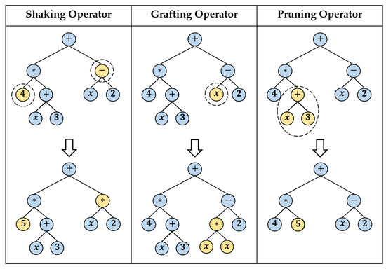
Figure 4.
Using shaking, grafting, and pruning operators to generate new trees from given ones.
2.2. Long Short-Term Memory (LSTM) Models
LSTMs are the most prominent RNNs models used for deep learning to solve time-series data prediction problems [36,37,40]. They are suitable for modeling and handling the temporal context among time-series data records. These deep learning models that have been introduced in [36] have gained popularity in the domain of time-series data predictions (speech recognition, gesture recognition, natural language processing, automatic translation, market stocks predictions, etc.). Figure 5 illustrates the main components of an LSTM unit as introduced originally by Hochreiter and Schmidhuber [36]. The main idea was to address vanishing/exploding gradients facing the researchers when the classical gradient descent-based back-propagation training algorithm on deep learning models [36,37]. A single basic cell of type LSTM, also named vanilla cell, includes an input gate, forget gate, and output gate. In addition, it contains a specific internal structure of individual hidden units. Those units and gates help in solving the vanishing/exploding effective back-propagation error over prolonged periods of time. The forget gate permits forgetting the non-important (non-discriminant) information, whereas the state of the cell permits remembering the most important information.
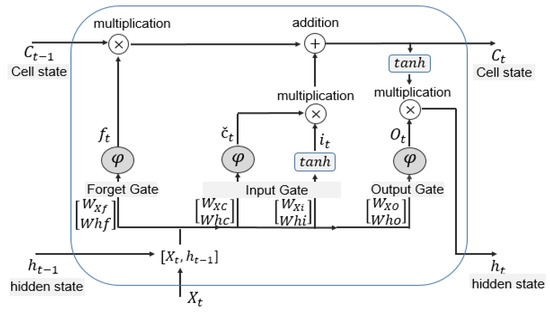
Figure 5.
The general structure of an LSTM unit with one input sign vector and one output .
An LSTM unit takes as input at instant a signal vector , the hidden state that depends on the output of the unit at instant , and the cell state of the LSTM unit at instant . The outputs of the cell consist of the current hidden state , the output of the cell at instant that will be used as an input in the next instant , and the cell state . In general, an LSTM unit has four sets of gates’ parameters and one set of output layer parameters. Those parameters are defined in the following five equations:
where D is the dimension of the input vector, H is the number of LSTM cells in a layer, and K is the number of classes in the case of classification. On the other hand, W(·) denotes the weight matrices, and b(·) represents the bias vectors that affect the transformation of a particular gate. Given an input vector, the forward pass can be described in the following seven equations.
The output of the forget gate is calculated using Equation (7). Then, the output of the input gate is calculated using Equation (8). The state of the cell is computed using Equations (9) and (10), consecutively. Finally, the output of the cell is found using Equations (11) and (12).
where , , , and denote outputs of the forget, input, output, and cell memory gates, respectively. The represents the sigmoid activation function defined by Equation (13), and ◦ stands for element-wise multiplication. The outcomes of the LSTM unit are (the state memory of the cell) and (the output value of the cell). These two outcomes are to be passed to the next time step. The reader can refer to [36] for more details about LSTM and other gated models.
3. Hybrid Approach Development
3.1. Building Base Models
The dataset used to design and validate the base predictors consists of weather and solar historical data provided by the AUMET solar and weather station at the American University of Middle East (AUM)—Kuwait. The dataset comprises daily data records with a resolution of 5 min. Each record (instance) includes up to 32 measures of weather and SR parameters. In this research, we have selected the most seven prominent parameters by using the PCA technique [41,42]:
- AirDensity (Kg/m3): the density of the air
- AirTemp_Avg (°C): the average temperature of the air 3 m above the surface
- HeatIndex (°C): the heat index
- RelativeWindSpeed_Max (m/s): the maximum relative wind speed
- RH_ Avg (%): the relative humidity in the air
- SurfaceTemp_Avg (°C): the average temperature 10 cm close to the surface
- SolarRadiation_Avg (W/m2): the average global solar radiation
We have built five LSTM individual models as base predictors of the GSR 15 min ahead. Each model is composed of a simple LSTM unit. All the base LSTM models have the same structure and activation functions. Moreover, we have used the same BPTT algorithm’s parameters to train the LSTM models in the first layer [35]. Each model receives as input a sequence of successive input vectors. In the experimental trials, we choose k = 2 based on a sensitivity analysis. Each of these vectors includes a subset of weather and solar parameters out of the total number of parameters described in the following paragraph. Each subset of the parameters includes the measured GSR and other selected weather parameters for k previous 15-min slots (windows). The resulting base models are as follows:
- LSTM_1 receives in each input vector the following parameters: Air Density, Max Relative Wind Speed, and Solar Radiation for the current and the previous 15-min slots.
- LSTM_2 receives in each input vector the following parameters: Air Density, Average Surface Temperature, and Solar Radiation for the current and the previous 15-min slots.
- LSTM_3 receives in each input vector the following parameters: Average Air Temperature, Heat Index, and Solar Radiation for the current and the previous 15-min slots.
- LSTM_4 receives in each input vector the following parameters: Average Air Temperature, Relative Humidity, and Solar Radiation for the current and the previous 15-min slots.
- LSTM_5 receives in each input vector the following parameters: Average Air Temperature, Average Surface Temperature, and Solar Radiation for the current and the previous 15-min slots.
The combinations mentioned earlier are the most performant in providing the best complementary information among the outputs of the individual predictors. That is a key factor to improve the overall prediction performance. In addition, we have designed and implemented a reference global LSTM model that receives all seven weather and solar radiation parameters in input to predict the solar radiation strength 15 min ahead.
LSTM_6 receives in each input vector all the adopted weather and solar parameters: Air Density, Average Air Temperature, Heat Index, Max Relative Wind Speed, Relative Humidity, Average Surface Temperature, and Solar Radiation for the current and the previous 15-min slots.
All the LSTM models use the same activation functions and the same parameters’ values in the BPTT training algorithm [36].
3.2. Building the Hybrid GP-LSTM Model
The hybrid LSTM-based GP approach consists of an ensemble of homogeneous LSTM-based predictors and a heuristic GP-based combiner. Two versions of the GP combiner have been examined, and they are set up as follows:
- A standard version consists of the primary mutation and crossover operators as is described in Section 2. The parameters of this version of GP module are setup as follows:
- ○
- The population size is set to be equal to 200 individuals. Each individual represents a nonlinear combination formula of the outputs of the base predictors.
- ○
- The set of operators that are used in the internal nodes of the trees that represent the individuals includes the four arithmetic operators: addition (+), difference (−), division (/), and multiplication (*). In addition, it includes the decimal log , the exponential function and the square root ().
- ○
- The depth of each of the trees that represent individuals is equal to eight. The maximum depth allowed for trees in each population is one of the adjustable parameters in a GP evolution process. The depth of each of the binary trees is set to be dynamic. It starts by an initial depth that can be dynamically increased until a selected maximum value is reached.
- ○
- The fitness function evaluates the efficiency of each of the individuals that represent candidate solutions (chromosomes). A fitness function related to the root mean square error (RMSE) has been used.
Moreover, some alternatives have been investigated and examined to adopt and set the following two parameters:
- ○
- The probability of applying each of the genetic operators (crossover and mutation).
- ○
- The sampling method to select individuals from the current population to participate in generating new individuals for the next generation.
- A hybrid version of the GP algorithm, named MP, consists of a local search module that permits selecting the best breeding among possible children from two crossover parents. The parameters of this version of GP module are setup almost the same as the standard one for comparison reasons. Therefore, the exact population sizes, set of operators, maximum depth, and fitness functions, and sampling methods have been adopted for this version.
3.3. Experiments Setup
3.3.1. Training and Testing Dataset
As we mentioned in Section 3.1, the dataset used to train and validate the base predictors consists of weather and solar historical data records. The dataset comprises daily data records with a resolution of 5 min. Our experiments have used the data records extracted for the period between September 2020 and March 2021 inclusive. We have removed the night hours from this dataset in which the SR strength is almost equal to 0 (absence of SR). The resolution of the data records has been decreased to be equal to 15 min. The resulted dataset that comprises 8854 data records has been divided into three subsets. The first subset is the one for training having the first 60% of the records to train the base predictors. The second subset is a hold-out subset having 20% of the dataset. This data set is dedicated to validate the base predictors and to design the heuristic GP model as we will describe in this section. The third subset contains the remaining 20% of the data records. The latter subset is the one for testing the base learners and the proposed GP-LSTM hybrid approach, and it has never been used in the training and validation phases.
The hold-out set is used as follows: After the training of the base predictors on the training subset (60% of the dataset), those predictors have been used to make predictions on the hold-out subset records, see Figure 6. So, we obtain five predicted values produced by the five base predictors for each instance in the hold-out subset. Therefore, we have created a new training set by considering these predicted values as input parameters to the GP model and by keeping the target values of the same hold-out subset. The GP heuristic model has been designed on this new training set by finding the best formula to combine the base predictors’ outputs to predict the target values of GSR 15-min ahead.
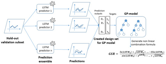
Figure 6.
Creating new training set for the GP-based combiner using the hold-out subset.
In order to reduce the noticeable difference in the scales adopted for the values of the weather and SR parameters, we have applied the MinMax scaling technique. The data values of parameters have been normalized to a standard scale using (14).
where is an original value sample of the parameter . min () and max () are the minimum and maximum measured values of the parameter respectively.
Finally, we have applied the sliding window technique to prepare the sequential inputs for each LSTM model in a pre-processing phase. During the training phase, the sliding window prepares the sequence of input vectors to include the data records on the 15-min slots of time before slot to predict the GSR for the slot . In this case, the input sequence contains the data records related to the 15-min sized slots , , …, until , and the output target is the GSR for the th period. The sliding window technique is shown in Figure 7.

Figure 7.
The sliding window technique to prepare time series input vectors.
The LSTM based predictors in the first layer of the model do not receive all the data parameters in each data record. Instead, each LSTM predictor gets a combination of selected parameters out of the seven parameters described in the previous paragraph. For example, one of the models receives the SR strength coupled with the Air Density and Heat Index measures for the current and the previous 15-min slots; another model receives the SR strength coupled with the Air Temperature, Relative Wind Speed measures for the current and previous 15-min, and so on. In our experiments, we have examined the effect of each input parameters’ combination on the performance of the base predictors.
3.3.2. Experiments
In our comparative analysis of the performance of the base predictors and the LSTM-GP hybrid approach, we examined two versions of the GP:
- A standard version of GP comprises the crossover operator with advanced versions of and mutation operators described in Section 2.1. This version is implemented in the GPLearn framework as described in Section 2.1.1.
- A standard version of MP that includes a local search sub-model that permits enhancing the exploitation capability of the GP model [27,28].
Plus, we decided to compare the performance of the GP-based combination in the post-processing module for the two versions as mentioned above of GP against machine learning stacking models. For that purpose, we designed and trained four machine learning models for the combination of type Random Forest [14], Multi-Layer Perceptron (MLP) [40], SVR [12,13], and K-Nearest Neighbors (KNN) [43]. All the stacking models have been trained on the training set used to design all the GP combiners. Each of those stacking models receives the prediction outputs of the LSTM predictors and makes the combination of those predictions using the experience that it gains during the training phase. In addition, we have used a simple averaging operator as a baseline reference combiner. The averaging operator receives the outputs of the base predictors and produces an averaging of those outputs. Figure 8 shows the pictogram of the GP-based combination of the LSTM base predictors.
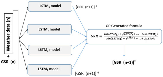
Figure 8.
The GP-LSTM hybrid model for combining LSTM models. Each individual predictor receives the weather and the GSR data of the current and the k previous 15-min slots to predict the GSR for the next 15-min slot.
In all experiments, we have used the Scikit-learn framework, developed in the French Institute for Research in Computer Science and Automation in France, [44] to implement, train, and validate all the examined predictors and combination models.
3.3.3. Evaluation Metrics
To evaluate and compare the performance of the base predictors and that of the proposed hybrid approach, we have used four statistical metrics, namely, the RMSE, the mean absolute error (MAE), the mean bias error (MBE), and the mean absolute percentage error (MAPE) [7]. We have evaluated the coefficient of determination between the observed and forecasted values of GSR energy.
Those metrics are computed as follows:
where is the predicted output and is the measured value related to that output.
All the above-described metrics are negatively oriented scores, which means that lower values are favorable.
The correlation coefficient is a numerical measure of the strength of the correlation between two variables [45]. The correlation coefficient is computed by Equation (19):
where and represents the average values of predicted and measured values, respectively.
Our experiments have used the coefficient of determination computed as the square of the correlation coefficient. The coefficient of determination shows percentage variation in a dependent y, which is expressed by all other independent x variables together. The higher value of is, the better. It is always between 0 and 1, so it can never be negative, since it is a squared value. It is easy to explain the square in terms of regression especially for multiple linear regression where numerous variables are involved [46].
4. Results and Discussion
In this work, we compared the performance of the heuristic GP techniques concerning the performance of stacking techniques in combining the outputs of base predictors of SR. The experimental study that we have conducted also investigated the improvement to the overall performance of those base predictors after employing the examined combination techniques. In the first stage, we have trained and tested the performance of the base predictors of the LSTM type that we have described in Section 2.2. Then, we have trained the GP-based combiners using the outputs of the base learners on the validation data subset. Finally, we have tested the overall prediction performance of the LSTM-GP hybrid models on the testing dataset. The same hold-out dataset that we have used to train the GP models has been used to train the combination performance of the stacking meta-models. The first row in Table 2 shows the obtained scores of evaluation metrics for the individual global LSTM model that receives all the weather and SR parameters as inputs. The following five rows show the scores of the same metrics obtained by the base predictors, where each of them receives a subset of the input parameters as described in Section 3.1. The best individual model in the ensemble is marked with ‘*’.

Table 2.
Results of individual models: underlined and bold scores indicate the best ones, and the best model is marked with ‘*’.
The results in Table 2 indicate that the LSTM_3 uses three parameters: namely Average Air Temperature, Heat Index, and SR have outperformed all the individual models and the global model that uses all the seven input parameters. The models LSTM_4 and LSTM_5 have also outperformed the individual global model. That means that each of these two individual models comprises enough information to outperform the global model.
Table 3 shows the obtained scores of the metrics for the combination models. The first row shows the scores for a simple averaging combiner. The next four rows show the scores of the metrics for the stacking combiners that employ machine learning techniques, and the last two rows show the values of the metrics scores for the LSTM_GP and LSTM_MP models.

Table 3.
Results of combination models of type simple averaging, machine learning-based stacking, and GP. Underlined and bold scores indicate the best ones.
The results in Table 3 indicate that the hybrid LSTM_GP models have outperformed all the stacking models and all the individual models reported in Table 2 in terms of all evaluation metrics. The LSTM_GP models have also outperformed the simple averaging model shown in the first line. The two versions of the GP hybrid models showed very close scores for the RSME and MAE metrics. These two hybrid models have exploited well the complementary information among the individual predictors of the committee. This last point can be explained by the negative and positive values of MBE for the individual models, which indicate that some of them underestimate and others overestimate the exact values of GSR. We believe that the advanced operators of mutation implemented in the GPLearn version have compensated the advantages of the local search in the MP hybrid model in solving the examined combination task.
The obtained scores for RMSE in Table 3 indicate that most of the examined combination models, especially the LSTM_GP and LSTM_MP hybrid models, have outperformed the global model that uses all the weather and SR parameters as input. It means that dividing the input parameters of the base learners into subsets in a pre-processing phase and then combining the complementary information of their outputs by a good combiner will ease the prediction task of those base learners and therefore improve the overall performance.
The sixth row in Table 3 shows that the standard GP combination model provides a decrease in the value of RMSE of the average outputs of individual LSTM models by almost 46.27%, as shown in (21):
The third, sixth, and seventh rows in Table 3 indicate that the two GP-based hybrid models LSTM_GP and LSTM_MP provide a decrease in the value of RMSE with respect to the best stacking combiner (LSTM_MLP with RMSE = 0.0337) by almost 29.37% and 31.15%, respectively, as shown in (22) and (23).
Figure 9 depicts the binary trees associated with the best individual candidate solutions in the last population of the standard GP and of the MP evolutionary computations. Each of These two best individuals represent the best combination formula for the outputs of the individual LSTMs’. Equation (24) represents the formula stored in the binary tree provided by the standard GP.
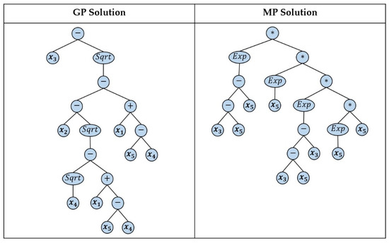
Figure 9.
Binary tree that represents the fittest individual in the last population of the standard GP evolutionary computation, and that represents the best combination formula that we have adopted in the hybrid GP_LSTM model, where x1 = LSTM_1, x2 = LSTM_2, x3 = LSTM_3, x4 = LSTM_4, and x5 = LSTM_5.
Figure 10 shows the daily average prediction error of GSR, 15 min ahead, which is provided by the simple averaging LSTM_Avg model, the stacking LSTM_MLP model, and the examined hybrid LSTM_GP model. To have a clear plot, we have considered the daily average errors of prediction related to of March 2021. The chart in Figure 10 shows a significant outperformance of the LSTM_GP model with respect to the other models in term of minimal deviation around the average value of the prediction error that is the closest to value 0.
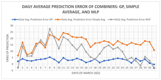
Figure 10.
The daily average prediction error of GSR of the simple average combiner, the best stacking model MLP, and standard GP combiner during March 2021.
5. Conclusions
In this study, we have discussed the short-term prediction of GSR strength on horizontals using hybrid solutions that combine the strength of LSTM models in modeling and predicting time-series data with the capability of GP techniques in finding nonlinear functions of combination. For that purpose, we have proposed and examined two versions of the GP heuristic technique of combination based on evolutionary computation: a standard version and another hybrid version, called Memetic Programming, that incorporates a local search sub-model to enhance the exploitation quality of the standard GP. To evaluate the performance of the proposed hybrid LSTM-GP approaches, an extensive experimental study that compares those approaches against stacking techniques has been conducted. The two versions of the GP hybrid approach have outperformed all the individual base predictors and most of the stacking techniques. That means that the GP-based heuristic modules in the hybrid approach have outperformed the stacking models in finding the best combination maps among the base predictors. Therefore, it can handle the complementary information among the outputs of those predictors. That is important, especially when the data available for designing and training the machine learning combiners (i.e., stacking) is small for practical reasons and therefore inadequate to adjust the freedom parameters of the stacking models.
Extending this study on predicting a different type of energy is one of the following perspectives of this work. Other future perspectives consist in applying the same hybrid techniques on ensembles of other gated recurrent models. In addition, and becasue the prediction performance of any ensemble of models depends on the excellent handling of complementary information among individual learners, finding convenient structures of combination is one of our interests in our future works.
Author Contributions
Conceptualization, R.A.-H., A.A., and M.F.; methodology, R.A.-H., M.F., and E.M.; software, R.A.-H., M.F., E.M.; validation, R.A.-H., E.M., and A.A; formal analysis, R.A.-H., M.F., A.A., and E.M.; investigation, R.A.-H., M.F., and E.M.; resources, R.A.-H., M.F., and E.M.; data curation, R.A.-H., M.F., and E.M.; writing—original draft preparation, R.A.-H., M.F., and A.A.; writing—review and editing, M.F., A.A.; visualization, R.A.-H., and M.F.; supervision, R.A.-H., A.A., and E.M. All authors have read and agreed to the published version of the manuscript.
Funding
This research received no external funding.
Data Availability Statement
The data used in this research is private and not publically available yet. The reader may ask for sample data directly from correspondent author by email.
Conflicts of Interest
The authors declare no conflict of interest.
Nomenclature
| GSR | Global Solar Radiation |
| LSTM | Long-Short Term Memory |
| RNN | Recurrent Neural Network |
| SR | Solar Radiation |
| GP | Genetic Programming |
| ANN | Artificial Neural Network |
| SVM | Support Vector Machines |
| RF | Random Forest |
| DT | Decision Tree |
| RT | Regression Tree |
| RMSE | Root Mean Square Error |
| ARIMA | Autoregressive Integrated Moving Average |
| MLR | Multilinear Regression |
| BDT | Bagged Decision Tree |
| BDTs | Bagging Decision Techniques |
| SVR | Support Vector Regressors |
| MP | Memetic Programming |
| LGP | Linear Genetic programming |
| MGGP | Multi-Gene Genetic Programming |
| Tpanel | Panel’s Temperature |
| NOCT | Nominal Operating Cell Temperature |
| NMOT | Nominal Module Operating Temperature |
| GEP | Gene Expression Programming |
| SA | Simulated Annealing |
| BPTT | Back-Propagation Through Time |
| GA | Genetic Algorithm |
| KNN | K-Nearest Neighbors |
| MAE | Mean Absolute Error |
| MBE | Mean Bias Error |
| MAPE | Mean Absolute Percentage Error |
| r | Correlation Coefficient |
| Coefficient of Determination |
References
- Vasylieva, T.; Lyulyov, O.; Bilan, Y.; Streimikiene, D. Sustainable economic development and greenhouse gas emissions: The dynamic impact of renewable energy consumption, GDP, and corruption. Energies 2019, 12, 3289. [Google Scholar] [CrossRef]
- Islam, M.T.; Huda, N.; Abdullah, A.B.; Saidur, R. A comprehensive review of state-of-the-art concentrating solar power (CSP) technologies: Current status and research trends. Renew. Sustain. Energy Rev. 2019, 91, 987–1018. [Google Scholar] [CrossRef]
- Diagne, M.; David, M.; Lauret, P.; Boland, J.; Schmutz, N. Review of solar irradiance forecasting methods and a proposition for small-scale insular grids. Renew. Sustain. Energy Rev. 2013, 27, 65–76. [Google Scholar] [CrossRef]
- Al-Hajj, R.; Assi, A.; Fouad, M.M. Forecasting Solar Radiation Strength Using Machine Learning Ensemble. In Proceedings of the 7th IEEE International Conference on Renewable Energy Research and Applications (ICRERA), Paris, France, 14–17 October 2018; pp. 184–188. [Google Scholar]
- Voyant, C.; Notton, G.; Kalogirou, S.; Nivet, M.L.; Paoli, C.; Motte, F.; Fouilloy, A. Machine learning methods for solar radiation forecasting: A review. Renew. Energy 2017, 105, 569–582. [Google Scholar] [CrossRef]
- Hou, M.; Zhang, T.; Weng, F.; Ali, M.; Al-Ansari, N.; Yaseen, Z.M. Global solar radiation prediction using hybrid online sequential extreme learning machine model. Energies 2018, 11, 3415. [Google Scholar] [CrossRef]
- Al-Hajj, R.; Assi, A.; Fouad, M. Short-Term Prediction of Global Solar Radiation Energy Using Weather Data and Machine Learning Ensembles: A Comparative Study. J. Sol. Energy Eng. 2021, 8, 1–38. [Google Scholar]
- Sharma, A.; Kakkar, A. Forecasting daily global solar irradiance generation using machine learning. Renew. Sustain. Energy Rev. 2018, 82, 2254–2269. [Google Scholar] [CrossRef]
- Yagli, G.M.; Yang, D.; Srinivasan, D. Automatic hourly solar forecasting using machine learning models. Renew. Sustain. Energy Rev. 2019, 105, 487–498. [Google Scholar] [CrossRef]
- Fan, J.; Wu, L.; Zhang, F.; Cai, H.; Zeng, W.; Wang, X.; Zou, H. Empirical and machine learning models for predicting daily global solar radiation from sunshine duration: A review and case study in China. Renew. Sustain. Energy Rev. 2019, 100, 186–212. [Google Scholar] [CrossRef]
- Li, P.; Bessafi, M.; Morel, B.; Chabriat, J.P.; Delsaut, M.; Li, Q. Daily surface solar radiation prediction mapping using artificial neural network: The case study of Reunion Island. ASME J. Sol. Energy Eng. 2020, 142, 021009. [Google Scholar] [CrossRef]
- Olatomiwa, L.; Mekhilef, S.; Shamshirband, S.; Mohammadi, K.; Petković, D.; Sudheer, C. A support vector machine–firefly algorithm-based model for global solar radiation prediction. Sol. Energy 2015, 115, 632–644. [Google Scholar] [CrossRef]
- Shang, C.; Wei, P. Enhanced support vector regression based forecast engine to predict solar power output. Renew. Energy 2018, 127, 269–283. [Google Scholar] [CrossRef]
- Piri, J.; Shamshirband, S.; Petković, D.; Tong, C.W.; Rehman, M.H. Prediction of the solar radiation on the earth using support vector regression technique. Infrared Phys. Technol. 2015, 68, 179–185. [Google Scholar] [CrossRef]
- Ren, Y.; Suganthan, P.N.; Srikanth, N. Ensemble methods for wind and solar power forecasting—A state-of-the-art review. Renew. Sustain. Energy Rev. 2015, 50, 82–91. [Google Scholar] [CrossRef]
- Wang, Z.; Srinivasan, R.S. Review of artificial intelligence based building energy use prediction: Contrasting the capabilities of single and ensemble prediction models. Renew. Sustain. Energy Rev. 2017, 75, 796–808. [Google Scholar] [CrossRef]
- Linares-Rodriguez, A.; Ruiz-Arias, J.A.; Pozo-Vazquez, D.; Tovar-Pescador, J. An artificial neural network ensemble model for estimating global solar radiation from Meteosat satellite images. Energy 2013, 61, 636–645. [Google Scholar] [CrossRef]
- Ahmed Mohammed, A.; Aung, Z. Ensemble learning approach for probabilistic forecasting of solar power generation. Energies 2016, 9, 1017. [Google Scholar] [CrossRef]
- Guo, J.; You, S.; Huang, C.; Liu, H.; Zhou, D.; Chai, J.; Black, C. An ensemble solar power output forecasting model through statistical learning of historical weather dataset. In Proceedings of the Power and Energy Society General Meeting (PESGM), Boston, MA, USA, 17–21 July 2016; pp. 1–5. [Google Scholar]
- Yeboah, F.E.; Pyle, R.; Hyeng, C.B.A. Predicting solar radiation for renewable energy technologies: A random forest approach. Int. J. Mod. Eng. 2015, 16, 100–107. [Google Scholar]
- Pan, C.; Tan, J. Day-Ahead Hourly Forecasting of Solar Generation Based on Cluster Analysis and Ensemble Model. IEEE Access 2019, 7, 112921–112930. [Google Scholar] [CrossRef]
- Basaran, K.; Özçift, A.; Kılınç, D. A New Approach for Prediction of Solar Radiation with Using Ensemble Learning Algorithm. Arab. J. Sci. Eng. Springer Sci. Bus. Media BV 2019, 44, 7159–7171. [Google Scholar] [CrossRef]
- Abuella, M.; Chowdhury, B. Random forest ensemble of support vector regression models for solar power forecasting. In Proceedings of the Power & Energy Society Innovative Smart Grid Technologies Conference (ISGT), Piscataway, NJ, USA, 23–26 April 2017; pp. 1–5. [Google Scholar]
- Poli, R.; Langdon, W.; McPhee, N. Genetic Programming: An Introductory Tutorial and a Survey of Techniques and Applications; Technical Report CES-475; University of Essex: Colchester, UK, 2007; ISSN 1744-8050. [Google Scholar]
- Poli, R.; Langdon, W.; McPhee, N. A Field Guide to Genetic Programming; Lulu Enterprises: Egham, UK, 2008; ISBN 1409200736. [Google Scholar]
- Riolo, R.; Vladislavleva, E.; Moore, J. Genetic Programming Theory and Practice IX; Springer Science & Business Media: Berlin, Germany, 2001; ISBN 1461417708. [Google Scholar]
- Mabrouk, E.; Hedar, A.; Fukushima, M. Memetic programming with adaptive local search using tree data structures. In Proceedings of the 5th International Conference on Soft Computing as Transdisciplinary Science and Technology, Paris, France, 28–31 October 2008; pp. 258–264. [Google Scholar]
- Mabrouk, E.; Hernández-Castro, J.C.; Fukushima, M. Prime number generation using memetic programming. Artif. Life Robot. 2010, 16, 53–56. [Google Scholar] [CrossRef][Green Version]
- Shavandi, H.; Ramyani, S.S. A linear genetic programming approach for the prediction of solar global radiation. Neural Comput. Appl. 2013, 23, 1197–1204. [Google Scholar] [CrossRef]
- Guven, A.; Aytek, A.; Yuce, M.I.; Aksoy, H. Genetic programming-based empirical model for daily reference evapotranspiration estimation. CLEAN Soil Air Water 2008, 36, 905–912. [Google Scholar] [CrossRef]
- Citakoglu, H.; Babayigit, B.; Haktanir, N.A. Solar radiation prediction using multi-gene genetic programming approach. Theor. Appl. Climatol. 2020, 142, 885–897. [Google Scholar] [CrossRef]
- Sohani, A.; Sayyaadi, H. Employing genetic programming to find the best correlation to predict temperature of solar photovoltaic panels. Energy Convers. Manag. 2020, 224, 113291. [Google Scholar] [CrossRef]
- Mostafavi, E.S.; Ramiyani, S.S.; Sarvar, R.; Moud, H.I.; Mousavi, S.M. A hybrid computational approach to estimate solar global radiation: An empirical evidence from Iran. Energy 2013, 49, 204–210. [Google Scholar] [CrossRef]
- Shiri, J.; Kim, S.; Kisi, O. Estimation of daily dew point temperature using genetic programming and neural networks approaches. Hydrol. Res. 2014, 45, 165–181. [Google Scholar] [CrossRef]
- Al-Hajj, R.; Assi, A. Estimating solar irradiance using genetic programming technique and meteorological records. AIMS Energy 2017, 5, 798–813. [Google Scholar] [CrossRef]
- Hochreiter, S.; Schmidhuber, J. Long short-term memory. Neural Comput. 1997, 9, 1735–1780. [Google Scholar] [CrossRef]
- Aslam, M.; Lee, J.M.; Kim, H.S.; Lee, S.J.; Hong, S. Deep Learning Models for Long-Term Solar Radiation Forecasting Considering Microgrid Installation: A Comparative Study. Energies 2020, 13, 147. [Google Scholar] [CrossRef]
- Srinivas, M.; Patnail, L. Genetic Algorithms: A Survey; IEEE Computer: Washington, DC, USA, 1994; Volume 27. [Google Scholar]
- GPlearn. Available online: https://gplearn.readthedocs.io/en/stable/intro.html (accessed on 21 May 2021).
- Haykin, S. Neural Networks and Learning Machines, 3rd ed.; Pearson, Prentice Hall: Delhi, India, 2010. [Google Scholar]
- Wold, S.; Esbensen, K.; Geladi, P. Principal component analysis. Chemom. Intell. Lab. Syst. 1987, 2, 37–52. [Google Scholar] [CrossRef]
- Karamizadeh, S.; Abdullah, S.M.; Manaf, A.A.; Zamani, M.; Hooman, A. An overview of principal component analysis. J. Signal Inf. Process. 2013, 4, 173. [Google Scholar] [CrossRef]
- Devroye, L.; Gyorfi, L.; Krzyzak, A.; Lugosi, G. On the strong universal consistency of nearest neighbor regression function estimates. Ann. Stat. 1994, 22, 1371–1385. [Google Scholar] [CrossRef]
- Pedregosa, F.; Varoquaux, G.; Gramfort, A.; Michel, V.; Thirion, B.; Grisel, O.; Vanderplas, J. Scikit-learn: Machine learning in Python. J. Mach. Learn. Res. 2011, 12, 2825–2830. [Google Scholar]
- Lee Rodgers, J.; Nicewander, W.A. Thirteen ways to look at the correlation coefficient. Am. Stat. 1988, 42, 59–66. [Google Scholar] [CrossRef]
- Zhang, D. A coefficient of determination for generalized linear models. Am. Stat. 2017, 71, 310–316. [Google Scholar] [CrossRef]
Publisher’s Note: MDPI stays neutral with regard to jurisdictional claims in published maps and institutional affiliations. |
© 2021 by the authors. Licensee MDPI, Basel, Switzerland. This article is an open access article distributed under the terms and conditions of the Creative Commons Attribution (CC BY) license (https://creativecommons.org/licenses/by/4.0/).