1. Introduction
Accurate forecasting of oil production is a significant and cumbersome task for monitoring and improving oil reservoirs. While hydrocarbons usage constitutes the largest share of the globe’s energy consumption in 2019, with over 58% world’s energy consumption [
1,
2]. Therefore, oil production forecasting plays a crucial role in the life cycle of oil reservoirs, including early resource evaluation and improving recovery. Simultaneously, various factors influence the hydrocarbon resources, including formation heterogeneities, the complexity of fluid flow within the subsurface formation, reservoir properties, and fluid properties that make the precise prediction of oil production more cumbersome [
3,
4]. Three approaches are frequently used to establish the prediction of oil production models in oil reservoirs. Numerical reservoir simulation (NRS) is considered the optimal traditional means for forecasting oil production. NRS method relies on a numerical model, which tends to achieve good performance and evaluate reservoir geological heterogeneity [
5,
6]. Furthermore, the NRS models have some limitations, including being time-consuming, cumbersome [
7], and it requires constructing an accurate static model, history matching, and other dynamic model parameters. Furthermore, analytical techniques are employed to compute various forms of wellbore flow rate adjustments. Depending on the reservoir heterogeneity, well structures complexity, and boundary conditions, some hypotheses are essential for determining the analytical solution [
8,
9,
10]. Moreover, the conventional decline curve analysis (DCA) technique [
11,
12] can forecast the production rate by evaluating the long-term hydrocarbon production data. The DCA approach employs the empirical equations to match the historical production data with a model, including harmonic, hyperbolic, and exponential models [
13]. These models are perfect curves and cannot consider the actual formation factors. Thus, it is challenging to ensure accurate performance by employing DCA.
The use of a numerical simulation to predict oil production is a more reliable and robust technique. Its accuracy is based on the accuracy of static models and history matching quality. However, it is troublesome to construct an accurate static model [
11,
14,
15]. Moreover, the parameterization techniques of the static model and the integrating method of objective components have a significant effect on history matching and reservoir prediction [
14,
15,
16]. Although multi-objective optimization can be determined, a perfect history matching model leads to poor prediction [
17]. Thus, the history matching approach is formidable and requires a long time, which renders a lot of work [
18].
The applications of deep learning (DL) and machine learning (ML) in the petroleum industry have gained more concern [
19], particularly in forecasting oil production [
20,
21], forecasting of pressure-volume-temperature (PVT) properties [
22,
23], optimizing well placement and oil production [
24,
25], the prediction of reservoir petrophysical properties, including porosity and permeability [
26,
27], and oil spill detection [
28]. Deep learning has been incorporated into the petroleum industry with the remarkable development of deep learning algorithms, enabling overcoming troublesome concerns in oilfields [
21].
Several DL and ML methods were introduced for forecasting oil production [
1,
20,
21]. For example, Sagheer et al. [
29] introduced Long Short-Term Memory (LSTM) to predict oil production time series. Fan et al. [
1] proposed to incorporate autoregressive integrated moving average (ARIMA) and LSTM to forecast oil production. In [
30], an optimized Random Vector Functional Link was introduced for time series forecasting. This model was implemented for oil production in Tahe oilfield. Liu et al. [
20] employed LSTM with Ensemble Empirical Mode Decomposition (EEMD) to predict oil production.
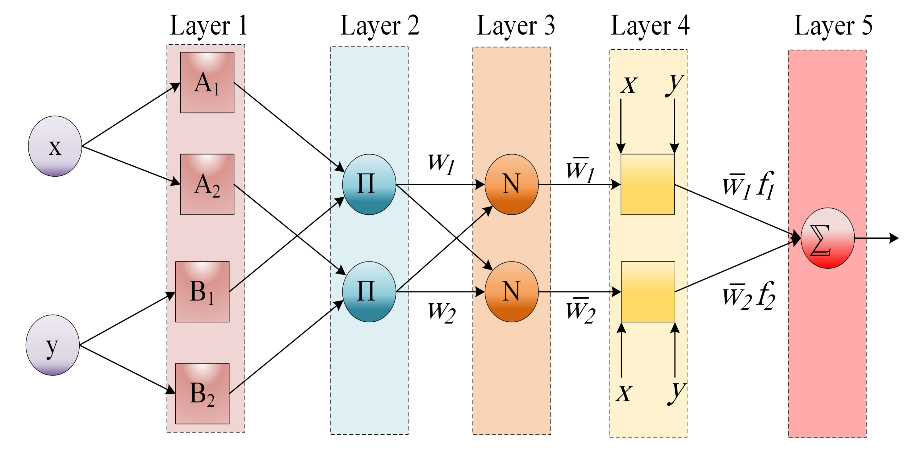
One of the most efficient time series prediction models is the Adaptive Neuro Fuzzy Inference System (ANFIS), which was employed for different forecasting problems [
31,
32,
33]. In this paper, we improve a modified ANFIS model using a new metaheuristic optimization algorithm called the Aquila Optimizer (AO) [
34]. It belongs to a class of nature-inspired optimization algorithms, which are motivated by the behavior of living organisms, such as grey wolves [
35], harris hawks [
36], or red foxes [
37]. The AO is inspired by the behavior of Aquila in nature, and it showed superior performance in solving different optimization and complex problems. In this paper, AO is applied to optimize ANFIS parameters to avoid traditional ANFIS shortcomings. First, the AO works by generating a set of candidates (solutions). Each one represents ANFIS parameter configurations. Then, each solution is evaluated using the training set. Thereafter, the solution that has the smallest fitness value is the best solution.
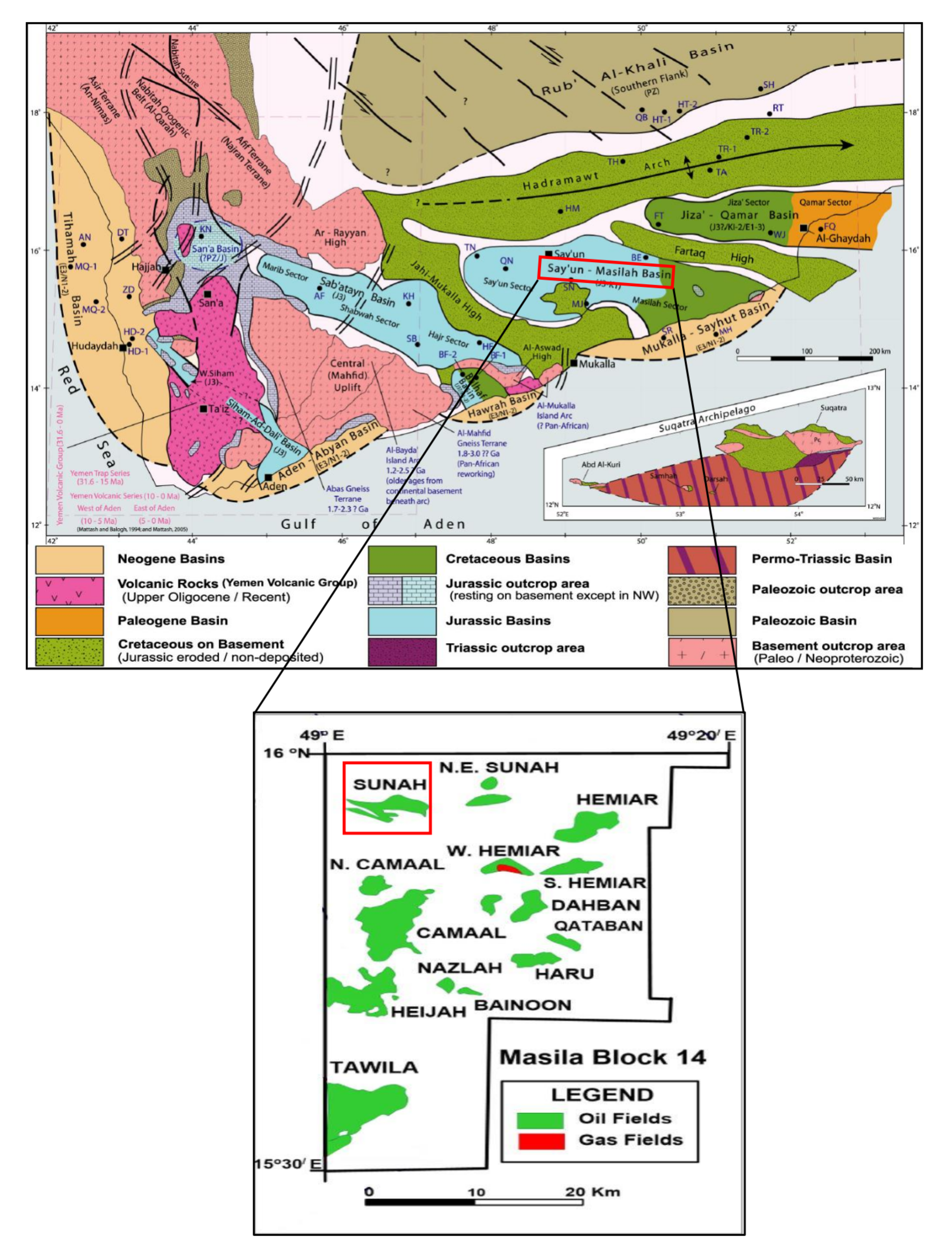
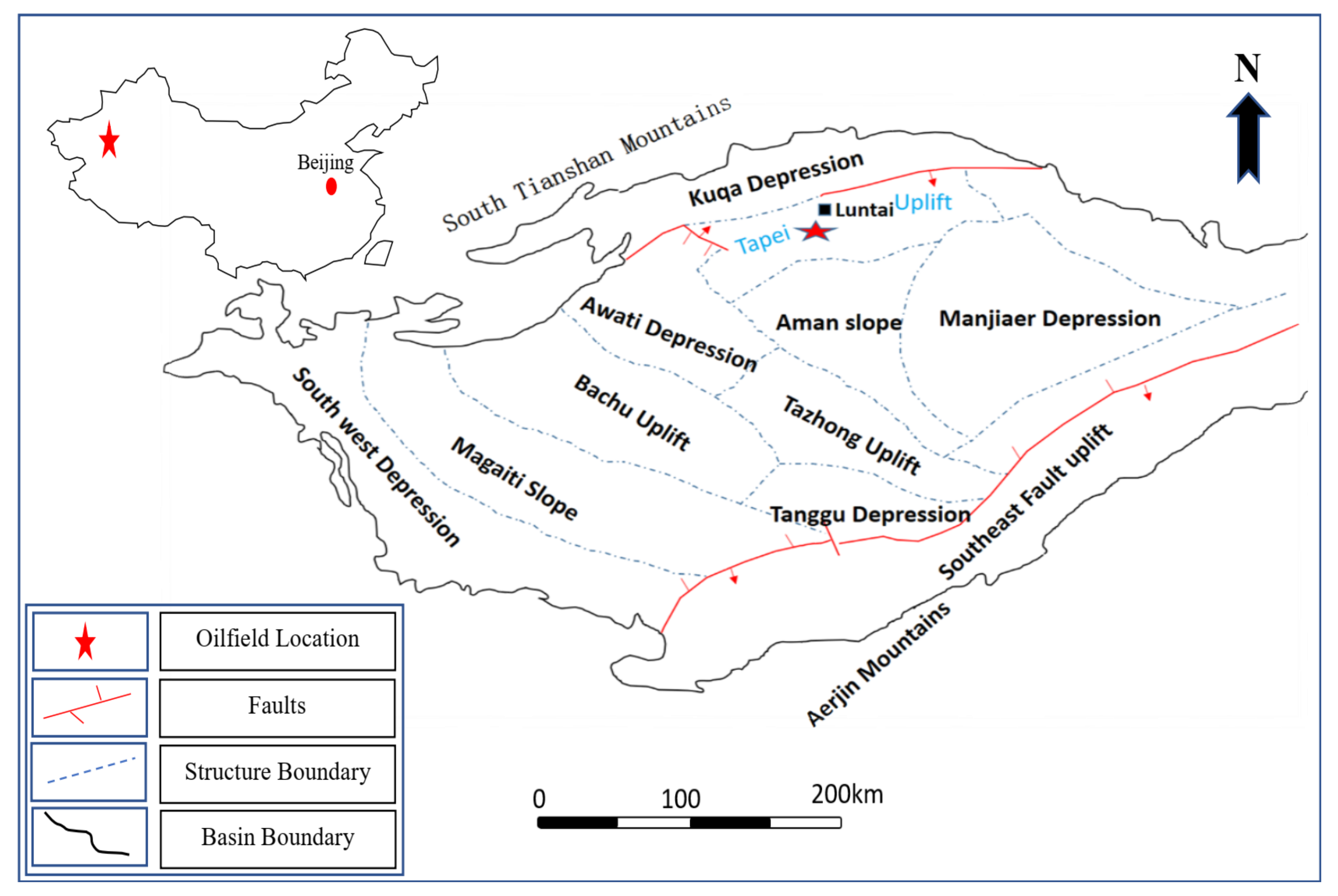
In this paper, AO-ANFIS is used on two real-world historical oil production datasets from Masila oilfields in Yemen and Tahe oilfields in China. The evaluation experiments are implemented using several performance measures, and extensive comparisons to several models are also carried out. The main contribution of the current study is:
A new modified ANFIS model, called AO-ANFIS, is proposed as a time series forecasting model for oil production.
The AO algorithm to optimize ANFIS parameters to overcome the shortcomings of ANFIS.
We implement extensive comparisons to several models to verify the performance of AO-ANFIS using two real-world datasets.
This paper is presented as:
Section 2 summarizes several oil forecasting studies. The backgrounds of applied methods are described in
Section 3. The AO-ANFIS time series forecasting model is described in
Section 4. Experiments and conclusion are presented in
Section 5 and
Section 6, respectively.
2. Related Work
In this section, we recap a list of relevant methods employed for oil production forecasting. Abdullayeva et al. [
38] established a hybrid model based on the integration of a Convolutional Neural Network (CNN) and LSTM networks, called CNN-LSTM, to forecast the oil production accurately. Calvette et al. [
39] implemented a deep learning algorithm in a proxy model to precisely duplicate the simulator by predicting the history data of production. Fan et al. [
1] proposed a hybrid model by incorporating the ARIMA model and LSTM to consider the impact of manual operation and assess the benefit of linearity and nonlinearity. Wang et al. [
40] proposed a hybridization forecasting model of the linear and non-linear to a modern predicting method in two stages. The first one, by incorporating between the grey model of the non-linear with the mentalism idea to establish non-linear metabolism grey model (NMGM). The second one by integrating the established NMGM with ARIMA to develop the NMGM-ARIMA method. In [
41], based on pressure-rate datasets, an integration model between non-linear autoregressive (NARX) and the LSTM was proposed to investigate synthetic datasets and contrast the findings of forecasting pressure. Zhong et al. [
42] proposed a deep learning proxy model to forecast the fluid saturation and reservoir pressure during the water flooding in heterogeneous reservoirs. Based on the recent development of deep learning, the coupled generative adversarial network (Co-GAN) was employed to determine the distribution of multidomain high-dimensional image data.
Wang et al. [
43] introduced a novel equal probability gene expression programming (EP-GEP) to eliminate the defects of the conventional Arps decline model in carbonate reservoir during the production decline analysis. The outcomes of the EP-GEP model show perfect forecasting accuracy with relative errors compared to the traditional methods. Yan et al. [
44] introduce time series data that can be examined with supervised algorithms and the Internet of Things (IoT). The elucidation of the efficiency of forecasting oil production techniques in steam flood scenarios was proposed. In addition, a 3% enhancement in oil production was observed based on the established optimal steam distribution plan. Singh et al. [
45] proposed a novel approach that can forecast the gas hydrate saturation(Sh) for any well utilizing various parameters, including bulk density, porosity, compressional wave (P wave) velocity well-logs neural networks (NNs), or without any well-specific calibration. The findings indicated that the accuracy of the established technique in forecasting (Sh) was 83%.
Zanjani et al. [
46] proposed various deep learning approaches, including Artificial Neural Network (ANN), Support Vector Regression (SVR), and Linear Regression (LR), to forecast the oil production. The findings indicate that all three approaches presented good forecasting. However, ANN is considered the optimal approach. Liu et al. [
47] proposed forecasting oil production, which considers the trends and the correlations of oil production data based on the LSTM approach. Alalimi et al. [
30] established an integrated model of Random Vector Functional Link (RVFL) and Spherical Search Optimizer (SSO) to forecast oil production from the Taha oilfield. The proposed model (SSO-RVFL) was evaluated with comparisons to several optimization methods. Sagheer et al. [
29] introduced deep LSTM as a deep learning technique to address the shortcomings of conventional forecasting methods and present accurate predictions.
4. Proposed AO-ANFIS Model
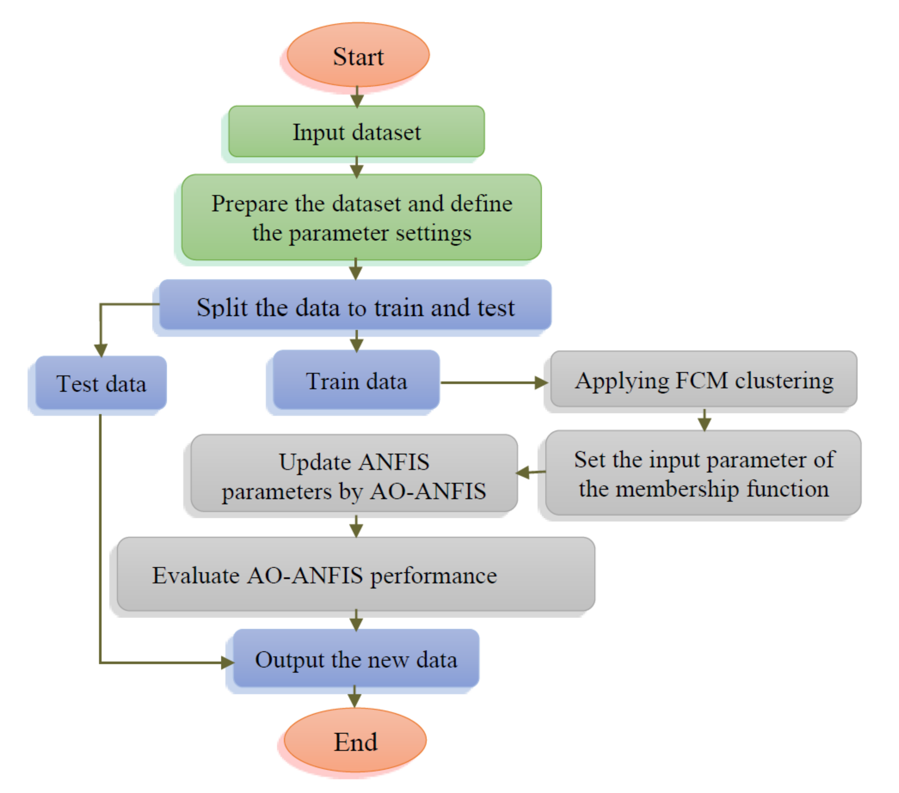
The framework of the developed forecasting oil production is given in
Figure 2. The developed model aims to enhance the ability of the ANFIS network for forecasting oil using the behavior of the AO algorithm. This is achieved by determining the optimal parameters of ANFIS using AO.
The developed AO-ANFIS starts by constructing the ANFIS network, followed by splitting the historical oil dataset into training and validation sets, which represent 70% and 30%, respectively. Then, the generation of a set of
N individuals
X, which represents the parameters for ANFIS (i.e., we have
N configurations). The next step is to use the training part of the dataset and compute the quality of each configuration using the following fitness function (i.e., it is the root mean square error):
where
T and
P refer to the actual and predicted output, respectively, and
is the number of training samples.
This process is followed by updating the value of the best configuration , and then updating other configurations using the operators of , as defined in Algorithm 1. Thereafter, the validation part is applied to the best configuration obtained so far and computed the quality of the output. Besides this quality, the proposed model is used for forecasting oil production.
The steps of the developed AO-ANFIS is given in Algorithm 2.
| Algorithm 2 Proposed AO-ANFIS algorithm |
| 1: Input: number of individuals (N) and total number of iterations (). |
| 2: Build the ANFIS network and generate set of N individuals X. |
| 3: Split the data into training and validation parts. |
| 4:
. |
| 5: while do |
| 6: Compute quality of each individual . |
| 7: Find (). |
| 8: Update other individuals using operators of AO as defined in Equations (8)–(15). |
| 9:
. |
| 10:
end while |
| 11:
Return . |
6. Conclusions
In the current study, we proposed a developed ANFIS model, called AO-ANFIS, for oil production time series forecasting. The Aquila Optimizer (AO) is a recently developed metaheuristic optimization algorithm that showed significant performance in addressing optimization tasks.
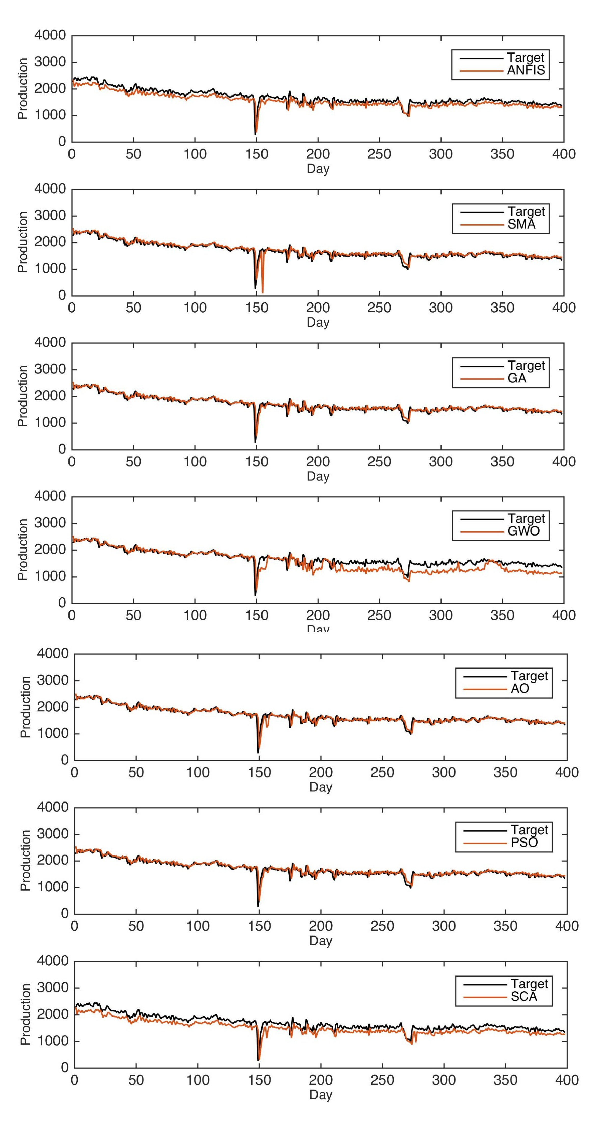
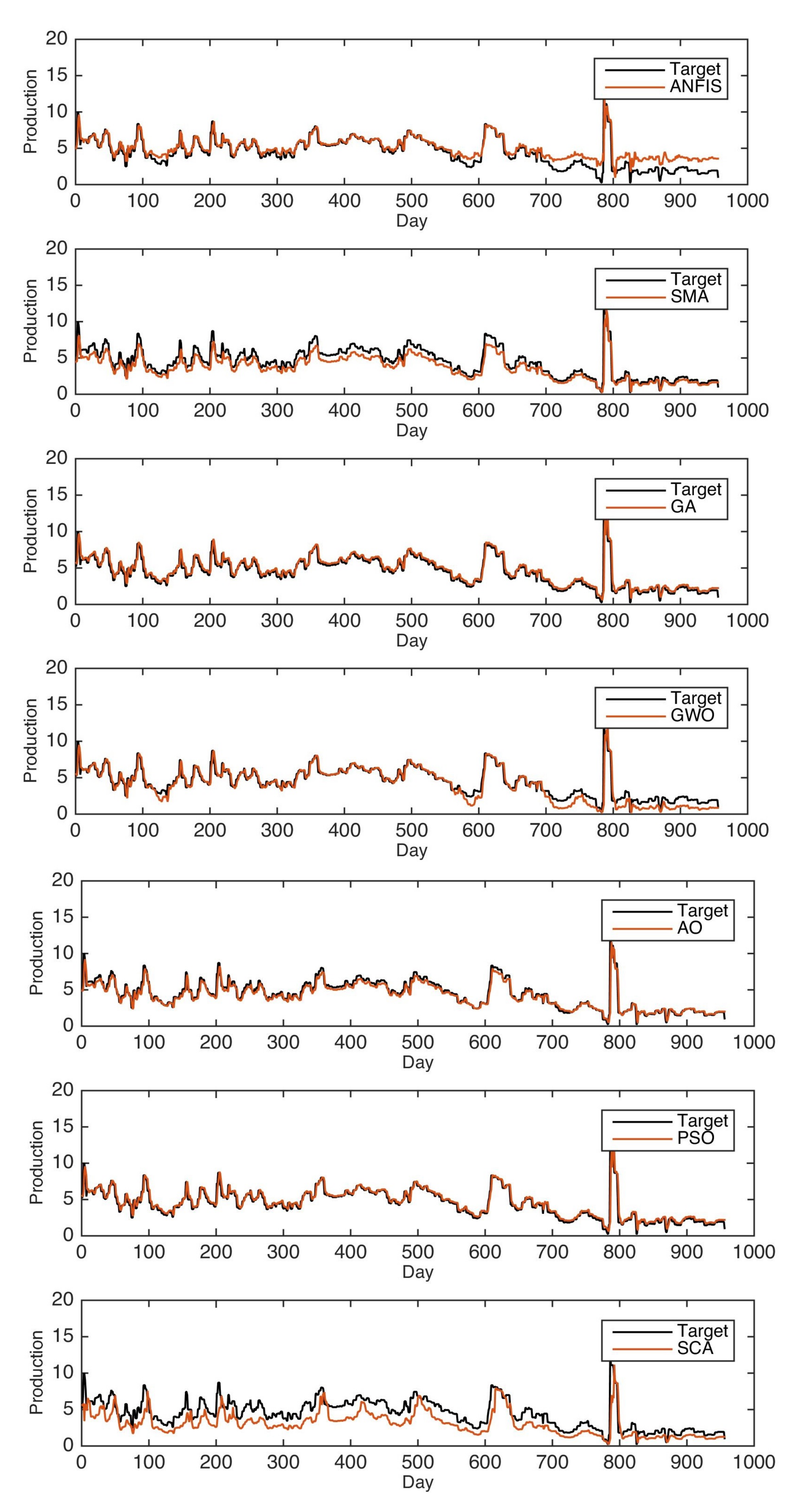
In this study, AO is applied to optimize ANFIS parameters to boost its prediction accuracy. The AO-ANFIS is evaluated with different datasets collected from two oilfields, namely, Tahe oilfields and Almasila oilfields, from China and Yemen, respectively. We also considered extensive experimental comparisons to state-of-art models, including the ANFIS traditional version, in addition to five modified versions of ANFIS using five optimization algorithms, called PSO, SCA, SSA, GWO, and SMA. AO-ANFIS has achieved significant results, and it outperformed the mentioned models in terms of RMSE, MAE, and .
The current AO-ANFIS model could be further developed to achieve more accurate results in future work. For example, applying a mutation strategy could further enhance the search process of the AO algorithm, which will result in improving ANFIS accuracy.


 ,
, 


