
An Imperfect Production–Inventory Model with Mixed Materials Containing Scrap Returns Based on a Circular Economy


Abstract
:1. Introduction
2. Notation and Assumptions
| System parameters: | |
| set-up and ordering costs per cycle. | |
| feed rate of new material in production in units. | |
| feed rate of scrap returns for product in units, where . | |
| production rate of finished product in units. | |
| demand rate for product in units, where . | |
| defective rate of finished product at stage, where | |
| maximum inventory level of scrap returns. | |
| maximum inventory level for product , where . | |
| inventory level of scrap returns when the stage of in-control transfers to out-of-control. | |
| inventory level of finished product when the stage of in-control transfers to out-of-control. | |
| holding cost of scrap returns per unit per unit time. | |
| holding cost of new material per unit per unit time. | |
| holding cost for a product per unit time, where . | |
| production, labor and inspection costs for a finished product. | |
| production cost for returning a defective product to scrap returns. | |
| opportunity cost for a unreturnable defective product , where . | |
| purchasing cost of material per unit. | |
| time period prior to depletion of inventory for product , , where . | |
| time period during in-control state, . | |
| Decision variables: | |
| production run time of product , , where . | |
| order quantity of new material per cycle. | |
| recovery rate of scrap returns. | |
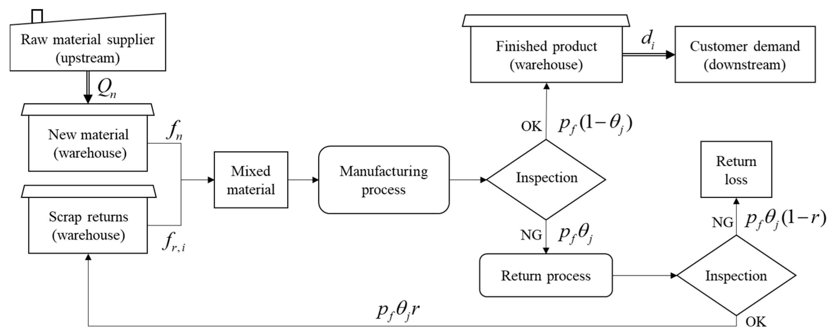
- The paired products with mixed materials containing scrap returns are considered in an imperfect production system. Figure 2 presents a schematic illustration of the proposed production system. From Figure 2, it can be seen that the processes and composition of mixed materials for two products are the same. Therefore, the production, labor, inspection, and material costs are also the same. The main material is ordered from a raw material supplier (upstream), and the order quantity is . The manufacturing process and return processes are both imperfect. Based on Rosenblatt and Lee [31], we assume that the manufacturing process may randomly shift from an in-control state to an out-of-control state, and the defective rate of finished product in the out-of-control state is higher than the in-control state, i.e., . The defective products from the manufacturing process forward to the return process, and the feed rate of defective product is , where . Only part of the defective products can be turned into scrap returns, and the production rate of scrap returns is , where . Note that the inspection time is so short that it can be disregarded.
- There are two products in the production system and the production sequence is product 1 to product 2. For product 1, the feed rate of scrap returns is less than or equal to the production rate of scrap returns to avoid the stage starves due to a lack of input from the previous stage, i.e., . For product 2, in order to avoid the unlimited accumulation of scrap returns, the feed rate of scrap returns must be higher than the production rate of scrap returns, i.e., . Based on the assumption , the following condition must be satisfied: . After rearranging the above inequality, it can be obtained that the reasonable range of recovery rate of scrap returns is . Note that the upper bound of must be less than or equal to 1, so which implies .
- The time period, , is a random variable that obeys a normal distribution with unknown mean and standard deviation . This paper adopts the lower confidence bound of mean to estimate the conservative value of by collecting the historical data.
- As far as we know, the production time of product 2 begins in the out-of-control period. The main reason is that the defective rate increases, and the feed rate of scrap returns must be faster to avoid the unlimited accumulation of scrap returns. Therefore, the production run time of product 1 must be higher than or equal to the length of time during the out-of-control period, i.e., .
- The recovery rate of scrap returns can be promoted through capital investment in return process improvement. Therefore, the capital investment can be treated as an increasing function of the recovery rate.
- Shortages are not allowed, and the following condition must be held: , where and .
3. Model Formulation
- R1.
- The maximum inventory level of scrap returns can be written asAfter rearranging the above equation, we obtain the following:
- R2.
- The maximum inventory level of the finished product 1 can be described as follows:After rearranging the above equation, we obtain the following:
- R3.
- The maximum inventory level of the finished product 2 can be described as follows:After rearranging the above equation, we obtain the following:
- R4.
- The ordering quantity of the material per cycle can also be described as the product of feed rate and total production time, i.e.,
- (a)
- Set-up and ordering costs (denoted by ): The set-up cost includes the costs associated with checking the initial output, adjusting the equipment, laying out the workplace, preparing the materials, preheating the boiler, etc. As to the ordering cost, it always includes delivery charges or the cost of labor required to place, receive, and stock an order. To facilitate the development of the model, set-up and ordering cost per cycle is treated as a fixed constant which implies .
- (b)
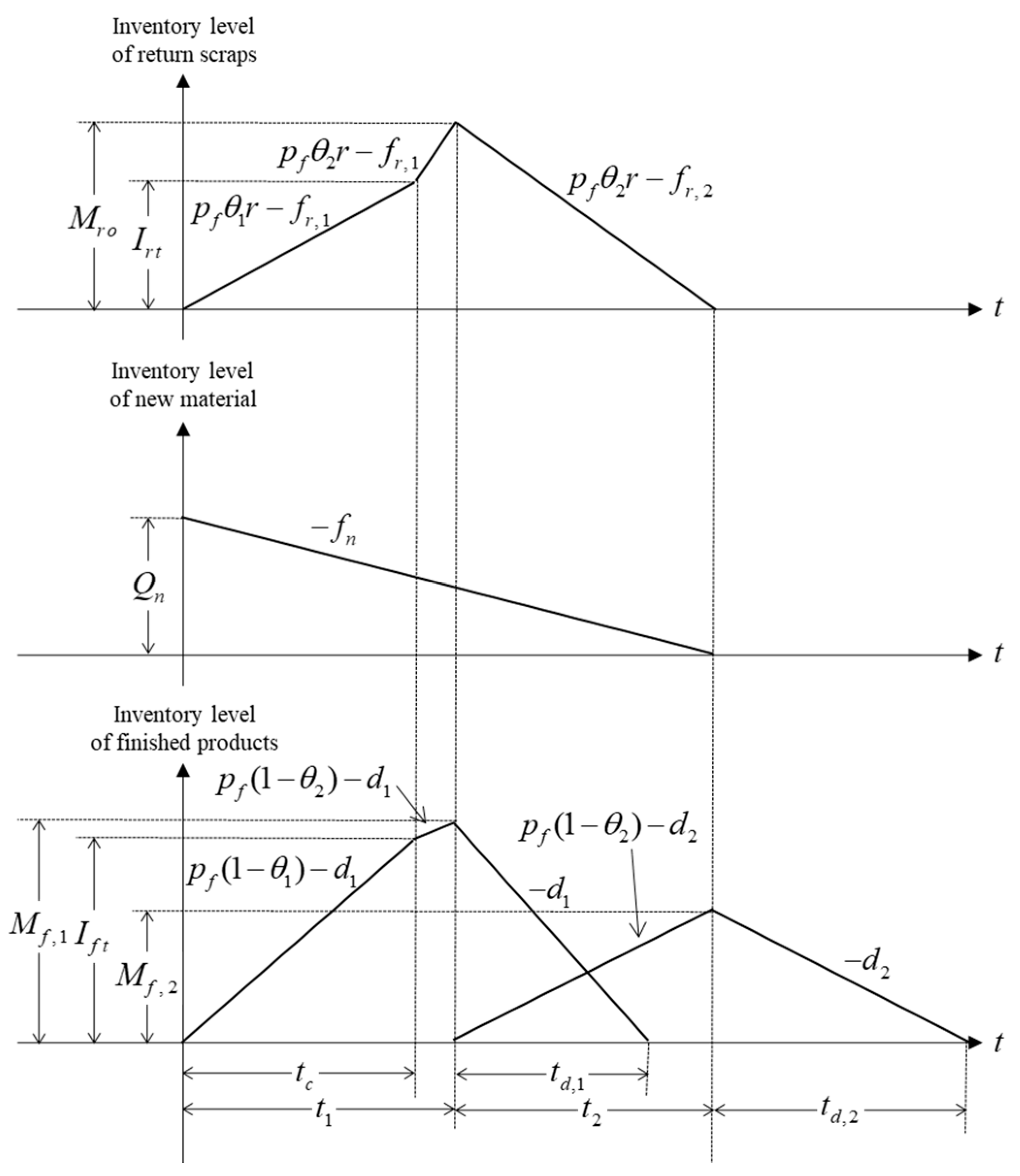
- Holding cost: From Figure 3, it is shown that this production system considers the stocks of scrap returns, new material, and two finished products. Each element of the holding cost per cycle is established as follows:
- (b-1)
- Holding cost of scrap returns (denoted by ):
- (b-2)
- Holding cost of new material (denoted by ):
- (b-3)
- Holding cost of finished product 1 (denoted by ):
- (b-4)
- Holding cost of finished product 2 (denoted by ):
- (c)
- Production cost (denoted by ): The production cost is the unit production cost for the finished product multiplied by the yield of the finished product, , which is:
- (d)
- Return cost for defective products (denoted by ): Due to the imperfect production system, defective products with units will be returned. As the unit cost per returned defective product is , the return cost for defective products per cycle is:
- (e)
- Opportunity cost due to lost return (denoted by ): This cost is the unit lost cost for the unreturnable defective product multiplied by the yield of the unreturnable defective product. The unreturnable volumes of products 1 and 2 per cycle are and , respectively. After multiplying the respective costs, the opportunity cost per cycle is:
- (f)
- Investment in converted equipment (denoted by ): The investment cost is an increasing function of recovery rate. In this paper, we consider an exponential form of investment function, which is:where denotes the percentage increase in per dollar increase in and is the original recovery rate of scrap returns.
- (g)
- Purchasing cost of material (denoted by ): This cost is the unit purchasing cost multiplied by the ordering quantity of material, which is:
| Algorithm 1 |
|
4. Application Example
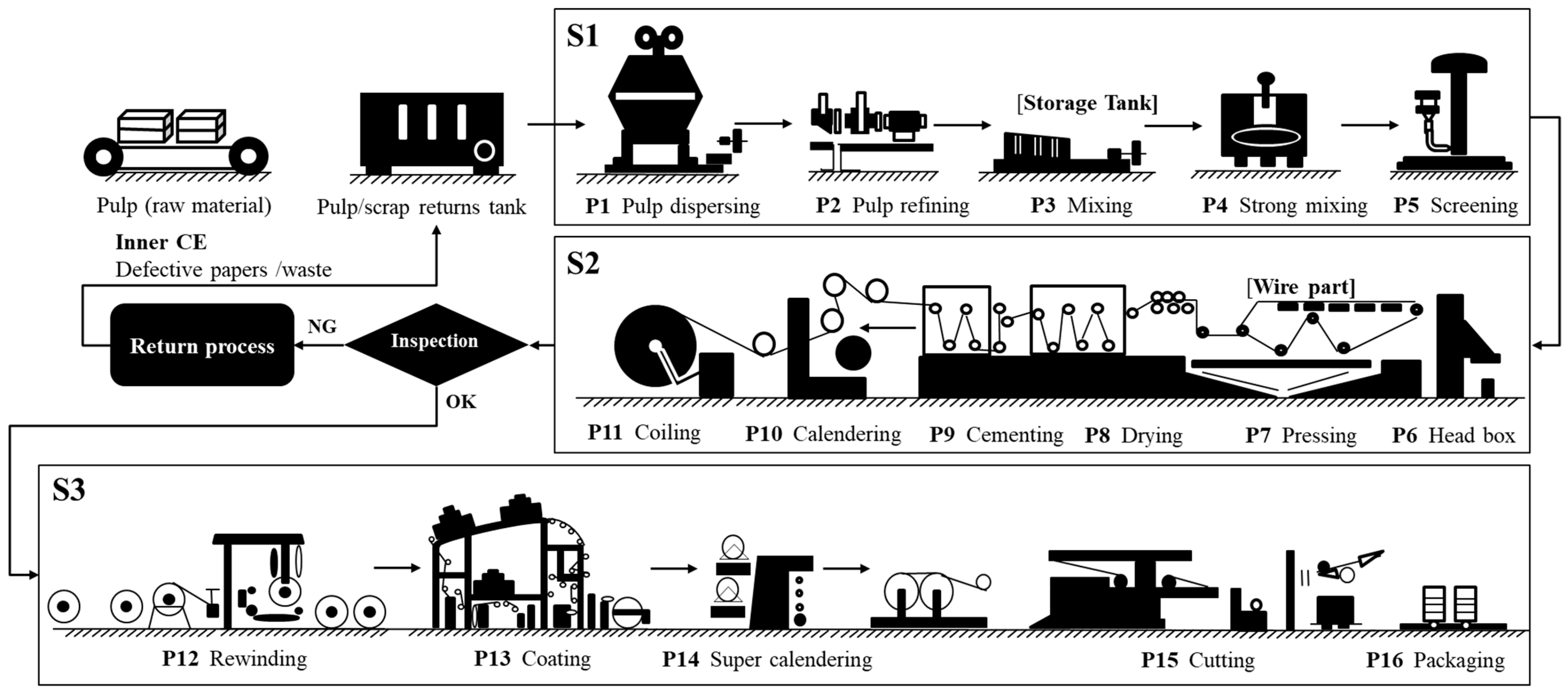
4.1. Pulp and Paper Industry
4.2. Numerical Example
- i.
- Demand of two products: 400 kg/day and 300 kg/day.
- ii.
- Operation for production and purchasing: $10,000/cycle, $10/kg, 600 kg/day, $5/kg, 100 kg/day, 2 kg/day and 40 kg/day.
- iii.
- Operation for stock: $0.6/kg/day, $0.4/kg/day $0.3/kg/day and $0.2/kg/day.
- iv.
- Defective rate of finished product: and .
- v.
- Operation for recovery activity: $2/kg, $0.15/kg, $0.1/kg, and .
- vi.
- Algorithm parameter: .
- vii.
- Time length of in-control period (): This paper considers a conservative estimate to express the value of due to the uncertainty of the time length of the in-control period. Assuming that the time length obeys a normal distribution, we use the lower confidence bound of time length (denoted by ) to express the conservative estimate under the confidence level, i.e.,where and for the given sample ; is quantile of Student’s T distribution with degrees of freedom. Table 2 presents historical data (28 cycles) of time length of in-control period (measured in days). First, we perform Anderson–Darling and Shapiro–Wilk normality tests with R software. The p-values in the two tests both exceed 0.1, i.e., there is no significant violation of the normal distribution. From Table 2, we calculate the sample mean 3.4979 days, sample standard deviation 0.0556 days and 3.4799 days with 95% confidence level, then let 3.4799 days.
4.3. Sensitivity Analysis
- M1.
- Increasing the cost parameters (, , , , , , , , or ) or decreasing the defective rate of finished product ( or ) would lead to an increase in the total cost per unit time. Moreover, the total cost per unit time is relatively sensitive to the product cost, the defective rate of finished product at out-of-control stage, and the holding cost of product 2. From the perspective of business operations, if companies want to effectively reduce total cost per unit time, they can start from these relatively high-sensitivity parameters.
- M2.
- In terms of holding cost parameters , , , and , increasing the values of the parameters led to corresponding decreases in , and except that an increase in causes increases in . It implies that the managers should shorten the length of the production cycle as holding costs increase. As to the exception of the impact of change on , the reason is the production sequence is product 1 to product 2 in the proposed model. When the value of increases, the manufacturer will shorten the length of the production cycle for product 1 and start producing product 2 ahead of schedule, resulting in an increase in the length of production cycle for product 2.
- M3.
- As the set-up and ordering cost increases, the values of , , , and increase. It’s intuitive that the quantity of materials ordered and the recovery rate of scrap returns each time will increase and that the length of the production cycle will be extended when the fixed cost increases.
- M4.
- With the increase in the value of cost parameter , , or , the optimal value of decreases while the optimal values of , , and increase.
- M5.
- All the optimal values of , , , and decrease as the value of or increases. This implies that the higher the oportunity cost for unreturnable defective product 2 or the defective rate of finished product at in-control stage, the shorter the length of production cycle and the lower recovery rate of scrap returns and the order quantity of material will be.
- M6.
- When the defective rate of finished product at out-of-control stage inceases, the value of will decrease at an increasing rate but the value of will increase at a decreasing rate such that the value of increases first and then decreases. Moreover, the recovery rate of scrap returns will be reduced when the defective rate of finished product at the out-of-control stage increases.
- M7.
- As the value of reproduction cost increases , the optimal values of and decrease but the optimal values of and increase. This implies that the defective products should be converted to scrap returns as much as possible for recycling due to high return costs. Note that the effect of this parameter change on the optimal solutions is the same as that of the holding cost .
- M8.
- For the investment in converted equipment, and decrease but , , and increase when the value of increases. It implies that the cost-effectiveness of the investment is worse with higher values of percentage increase in investment capital to improve the recovery rate of scrap returns.
5. Conclusions
Author Contributions
Funding
Institutional Review Board Statement
Informed Consent Statement
Data Availability Statement
Acknowledgments
Conflicts of Interest
References
- Taft, E.W. The Most Economical Production Lot. Iron Age 1918, 101, 1410–1412. [Google Scholar]
- Darwish, M.; Ben-Daya, M. Effect of Inspection Errors and Preventive Maintenance on a Two-Stage Production Inventory system. Int. J. Prod. Econ. 2007, 107, 301–313. [Google Scholar] [CrossRef]
- Lee, H.-H. The Investment Model in Preventive Maintenance in Multi-Level Production Systems. Int. J. Prod. Econ. 2008, 112, 816–828. [Google Scholar] [CrossRef]
- Pearn, W.L.; Su, R.H.; Weng, M.W.; Hsu, C.H. Optimal Production Run Time for Two-Stage Production System with Imperfect Processes and Allowable Shortages. Central Eur. J. Oper. Res. 2010, 19, 533–545. [Google Scholar] [CrossRef]
- Sarker, B.R.; Jamal, A.; Mondal, S. Optimal Batch Sizing in a Multi-Stage Production System with Rework Consideration. Eur. J. Oper. Res. 2008, 184, 915–929. [Google Scholar] [CrossRef]
- Cárdenas-Barrón, L.E. On Optimal Batch Sizing in a Multi-Stage Production System with Rework Consideration. Eur. J. Oper. Res. 2009, 196, 1238–1244. [Google Scholar] [CrossRef]
- Chang, H.-J.; Su, R.-H.; Yang, C.-T.; Weng, M.-W. An economic Manufacturing Quantity Model for a Two-Stage Assembly System with Imperfect Processes and Variable Production Rate. Comput. Ind. Eng. 2012, 63, 285–293. [Google Scholar] [CrossRef]
- Sarkar, S.; Shewchuk, J.P. Use of Advance Demand Information in Multi-Stage Production-Inventory Systems with Multiple Demand Classes. Int. J. Prod. Res. 2013, 51, 57–68. [Google Scholar] [CrossRef]
- Paul, S.K.; Sarker, R.; Essam, D. A Disruption Recovery Plan in a Three-Stage Production-Inventory System. Comput. Oper. Res. 2015, 57, 60–72. [Google Scholar] [CrossRef]
- Wang, Z.; Chan, F.T.S.; Li, M. A Robust Production Control Policy for Hedging Against Inventory Inaccuracy in a Multiple-Stage Production System with Time Delay. IEEE Trans. Eng. Manag. 2018, 65, 474–486. [Google Scholar] [CrossRef]
- Su, R.-H.; Weng, M.-W.; Huang, Y.-F. Innovative Maintenance Problem in a Two-Stage Production-Inventory System with Imperfect Processes. Ann. Oper. Res. 2019, 287, 379–401. [Google Scholar] [CrossRef]
- Su, R.-H.; Weng, M.-W.; Yang, C.-T. Effects of Corporate Social Responsibility Activities in a Two-Stage Assembly Production System with Multiple Components and Imperfect Processes. Eur. J. Oper. Res. 2020, 293, 469–480. [Google Scholar] [CrossRef]
- Chiu, Y.-S.P.; Huang, C.-C.; Wu, M.-F.; Chang, H.-H. Joint Determination of Rotation Cycle Time and Number of Shipments for a Multi-Item EPQ Model with Random Defective Rate. Econ. Model. 2013, 35, 112–117. [Google Scholar] [CrossRef]
- Sarkar, B.; Cárdenas-Barrón, L.E.; Sarkar, M.; Singgih, M.L. An Economic Production Quantity Model with Random Defective Rate, Rework Process and Backorders for a Single Stage Production System. J. Manuf. Syst. 2014, 33, 423–435. [Google Scholar] [CrossRef]
- Tayyab, M.; Sarkar, B. Optimal Batch Quantity in a Cleaner Multi-Stage Lean Production System with Random Defective Rate. J. Clean. Prod. 2016, 139, 922–934. [Google Scholar] [CrossRef]
- Kang, C.W.; Ullah, M.; Sarkar, B.; Hussain, I.; Akhtar, R. Impact of Random Defective Rate on Lot Size Focusing Work-In-Process Inventory in Manufacturing System. Int. J. Prod. Res. 2017, 55, 1748–1766. [Google Scholar] [CrossRef]
- Sarkar, B.; Dey, B.K.; Pareek, S.; Sarkar, M. A Single-Stage Cleaner Production System with Random Defective Rate and Remanufacturing. Comput. Ind. Eng. 2020, 150, 106861. [Google Scholar] [CrossRef]
- Chung, C.-J.; Widyadana, G.A.; Wee, H.M. Economic Production Quantity Model for Deteriorating Inventory with Random Machine Unavailability and Shortage. Int. J. Prod. Res. 2011, 49, 883–902. [Google Scholar] [CrossRef]
- Widyadana, G.A.; Wee, H.M. Optimal Deteriorating Items Production Inventory Models with Random Machine Breakdown and Stochastic Repair Time. Appl. Math. Model. 2011, 35, 3495–3508. [Google Scholar] [CrossRef]
- Öztürk, H. Modeling an Inventory Problem with Random Supply, Inspection and Machine Breakdown. Opsearch 2019, 56, 497–527. [Google Scholar] [CrossRef]
- Öztürk, H. Optimal Production Run Time for an Imperfect Production Inventory System with rework, Random Breakdowns and Inspection Costs. Oper. Res. 2021, 21, 167–204. [Google Scholar] [CrossRef]
- Pal, B.; Adhikari, S. Random Machine Breakdown and Stochastic Corrective Maintenance Period on an Economic Production Inventory Model with Buffer Machine and Safe Period. RAIRO Oper. Res. 2021, 55, S1129–S1149. [Google Scholar] [CrossRef]
- Chiu, Y.-S.P.; Wu, C.-S.; Wu, H.Y.; Chiu, S.W. Studying the Effect of Stochastic Breakdowns, Overtime, and Rework on Inventory Replenishment Decision. Alex. Eng. J. 2021, 60, 1627–1637. [Google Scholar] [CrossRef]
- Sarkar, B. An Inventory Model with Reliability in an Imperfect Production Process. Appl. Math. Comput. 2012, 218, 4881–4891. [Google Scholar] [CrossRef]
- Li, N.; Chan, F.T.S.; Chung, S.H.; Tai, A.H. A Stochastic Production-Inventory Model in a Two-State Production System with Inventory Deterioration, Rework Process, and Backordering. IEEE Trans. Syst. Man Cybern. Syst. 2016, 47, 916–926. [Google Scholar] [CrossRef]
- Mahata, G.C. A Production-Inventory Model with Imperfect Production Process and Partial Backlogging under Learning Considerations in Fuzzy Random Environments. J. Intell. Manuf. 2014, 28, 883–897. [Google Scholar] [CrossRef]
- Huang, H.; He, Y.; Li, D. Coordination of Pricing, Inventory, and Production Reliability Decisions in Deteriorating Product Supply Chains. Int. J. Prod. Res. 2018, 56, 6201–6224. [Google Scholar] [CrossRef]
- Dey, B.K.; Sarkar, B.; Sarkar, M.; Pareek, S. An Integrated Inventory Model Involving Discrete Setup Cost Reduction, Variable Safety Factor, Selling Price Dependent Demand, and Investment. RAIRO Oper. Res. 2019, 53, 39–57. [Google Scholar] [CrossRef] [Green Version]
- Manna, A.K.; Das, B.; Tiwari, S. Impact of Carbon Emission on Imperfect Production Inventory System with Advance Payment Base Free Transportation. RAIRO Oper. Res. 2020, 54, 1103–1117. [Google Scholar] [CrossRef]
- Dey, B.K.; Pareek, S.; Tayyab, M.; Sarkar, B. Autonomation Policy to Control Work-in-Process Inventory in a Smart Production System. Int. J. Prod. Res. 2021, 59, 1258–1280. [Google Scholar] [CrossRef]
- Rosenblatt, M.J.; Lee, H.L. Economic Production Cycles with Imperfect Production Processes. IIE Trans. 1986, 18, 48–55. [Google Scholar] [CrossRef]
- Love, P. Influence of Project Type and Procurement Method on Rework Costs in Building Construction Projects. J. Constr. Eng. Manag. 2002, 128, 18–29. [Google Scholar] [CrossRef] [Green Version]
- Geissdoerfer, M.; Savaget, P.; Bocken, N.M.P.; Hultink, E.J. The Circular Economy—A new sustainability paradigm? J. Clean. Prod. 2017, 143, 757–768. [Google Scholar] [CrossRef] [Green Version]
- MacArthur, E. Towards the Circular Economy, Economic and Business Rationale for an Accelerated Transition; Ellen MacArthur Foundation: Cowes, UK, 2013; pp. 21–34. [Google Scholar]
- Geissdoerfer, M.; Pieroni, M.P.; Pigosso, D.C.; Soufani, K. Circular Business Models: A review. J. Clean. Prod. 2020, 277, 123741. [Google Scholar] [CrossRef]
- Cambini, A.; Martein, L. Generalized Convexity and Optimization. Mult. Criteria Decis. Mak. 2009, 616. [Google Scholar] [CrossRef]
- How do we Make Pulp and Paper? Available online: http://www.chp.com.tw/en/product/product_learn (accessed on 16 July 2021).


| Literatures | Stage | Imperfect Process | Disposal Ways | |||||
|---|---|---|---|---|---|---|---|---|
| CD | RD | RB | RS | RW | SP | PD | ||
| Darwish and Ben-Daya [2] | MS | V | V | |||||
| Lee [3] | MS | V | V | |||||
| Sarker et al. [5] | MS | V | V | |||||
| Cárdenas-Barrón [6] | MS | V | V | |||||
| Pearn et al. [4] | MS | V | V | |||||
| Chung et al. [18] | SS | V | V | |||||
| Widyadana and Wee [19] | SS | V | V | |||||
| Chang et al. [7] | MS | V | V | |||||
| Sarkar [24] | SS | V | V | |||||
| Sarkar and Shewchuk [8] | MS | |||||||
| Chiu et al. [13] | SS | V | V | |||||
| Sarkar et al. [14] | SS | V | V | |||||
| Paul et al. [9] | MS | |||||||
| Tayyab and Sarkar [15] | MS | V | V | |||||
| Kang et al. [16] | SS | V | V | V | ||||
| Li et al. [25] | SS | V | V | V | ||||
| Mahata [26] | SS | V | V | |||||
| Wang et al. [10] | MS | V | ||||||
| Huang et al. [27] | SS | V | V | |||||
| Öztürk [20] | SS | V | V | V | ||||
| Dey et al. [28] | SS | V | V | |||||
| Su et al. [11] | MS | V | V | |||||
| Sarkar et al. [17] | SS | V | V | |||||
| Manna et al. [29] | SS | V | V | V | ||||
| Su et al. [12] | MS | V | V | |||||
| Öztürk [21] | SS | V | V | V | ||||
| Pal and Adhikari [22] | SS | V | ||||||
| Chiu et al. [23] | SS | V | V | |||||
| Dey et al. [30] | SS | V | V | |||||
| 3.57 | 3.60 | 3.58 | 3.48 | 3.49 | 3.54 | 3.43 |
| 3.55 | 3.54 | 3.48 | 3.50 | 3.51 | 3.52 | 3.41 |
| 3.43 | 3.49 | 3.41 | 3.43 | 3.54 | 3.48 | 3.50 |
| 3.56 | 3.54 | 3.41 | 3.52 | 3.41 | 3.52 | 3.50 |
| Parameters | % Change | % Change in | ||||
|---|---|---|---|---|---|---|
| −50 | −7.3178 | −15.5275 | −2.6008 | −11.9357 | −2.7382 | |
| −25 | −3.4228 | −7.3825 | −1.1727 | −5.6504 | −1.3214 | |
| 25 | 3.0781 | 6.8053 | 0.9930 | 5.1744 | 1.2452 | |
| 50 | 5.8900 | 13.1525 | 1.8513 | 9.9756 | 2.4275 | |
| −50 | 0.0186 | −0.0403 | −0.0236 | −0.0145 | −0.0105 | |
| −25 | 0.0093 | −0.0201 | −0.0118 | −0.0072 | −0.0052 | |
| 25 | −0.0093 | 0.0209 | 0.0118 | 0.0072 | 0.0052 | |
| 50 | −0.0197 | 0.0411 | 0.0236 | 0.0145 | 0.0105 | |
| −50 | 0.0021 | 0.0040 | 0.0007 | 0.0032 | −0.0110 | |
| −25 | 0.0010 | 0.0024 | 0.0002 | 0.0014 | −0.0056 | |
| 25 | −0.0010 | −0.0016 | −0.0002 | −0.0014 | 0.0056 | |
| 50 | −0.0021 | −0.0032 | −0.0005 | −0.0027 | 0.0110 | |
| −50 | 4.3815 | −22.7868 | −11.2685 | −10.9027 | −34.6177 | |
| −25 | 2.1970 | −11.0931 | −5.1614 | −5.2795 | −17.1267 | |
| 25 | −2.2343 | 10.6093 | 4.4686 | 4.9910 | 16.8248 | |
| 50 | −4.5141 | 20.8136 | 8.4100 | 9.7346 | 33.3928 | |
| −50 | 0.3686 | −1.8122 | −0.8062 | −0.8587 | −2.8321 | |
| −25 | 0.1843 | −0.9041 | −0.4019 | −0.4280 | −1.4150 | |
| 25 | −0.1843 | 0.9017 | 0.3972 | 0.4262 | 1.4129 | |
| 50 | −0.3696 | 1.7993 | 0.7873 | 0.8505 | 2.8238 | |
| −50 | 0.2247 | −0.1385 | −0.1466 | 0.0204 | −0.6254 | |
| −25 | 0.1118 | −0.0692 | −0.0733 | 0.0100 | −0.3126 | |
| 25 | −0.1118 | 0.0692 | 0.0733 | −0.0100 | 0.3126 | |
| 50 | −0.2226 | 0.1377 | 0.1466 | −0.0199 | 0.6251 | |
| −50 | 6.5226 | −1.8340 | −3.4307 | 1.8216 | −1.6250 | |
| −25 | 2.9621 | −0.9524 | −1.6172 | 0.7600 | −0.7896 | |
| 25 | −2.5262 | 1.0104 | 1.4683 | −0.5362 | 0.7507 | |
| 50 | −4.7201 | 2.0698 | 2.8207 | −0.9004 | 1.4678 | |
| −50 | 8.8097 | 46.3055 | 9.3912 | 29.9032 | −4.2432 | |
| −25 | 3.7842 | 17.5659 | 4.0218 | 11.5372 | −1.8803 | |
| 25 | −2.9642 | −12.0721 | −3.2368 | −8.0874 | 1.5741 | |
| 50 | −5.3589 | −20.9859 | −5.9558 | −14.1500 | 2.9340 | |
| −50 | 5.7948 | 8.7399 | 0.5012 | 7.4516 | −1.9371 | |
| −25 | 2.7447 | 4.1614 | 0.2530 | 3.5417 | −0.9520 | |
| 25 | −2.4879 | −3.8032 | −0.2601 | −3.2278 | 0.9221 | |
| 50 | −4.7594 | −7.2956 | −0.5202 | −6.1857 | 1.8169 | |
| −50 | 0.3417 | 0.3921 | −0.0118 | 0.3700 | −0.0960 | |
| −25 | 0.1698 | 0.1956 | −0.0047 | 0.1843 | −0.0479 | |
| 25 | −0.1688 | −0.1940 | 0.0047 | −0.1834 | 0.0479 | |
| 50 | −0.3365 | −0.3880 | 0.0118 | −0.3655 | 0.0955 | |
| −50 | −21.1830 | 3.0738 | 11.2685 | −7.5372 | −3.9855 | |
| −25 | −9.1110 | 1.4870 | 4.6672 | −3.1490 | −1.7307 | |
| 25 | 7.3654 | −1.4008 | −3.6198 | 2.4343 | 1.4229 | |
| 50 | 13.5639 | −2.7292 | −6.5800 | 4.3981 | 2.6404 | |
| −50 | 9.7197 | 4.0157 | 1.3997 | 6.5109 | 1.2767 | |
| −25 | 4.8619 | 1.9974 | 0.7046 | 3.2505 | 0.6382 | |
| 25 | −4.8650 | −1.9748 | −0.7164 | −3.2391 | −0.6380 | |
| 50 | −9.7322 | −3.9255 | −1.4399 | −6.4656 | −1.2756 | |
| −50 | 35.6414 | −62.0053 | −4.9249 | −19.2904 | 16.2904 | |
| −25 | 29.2203 | −25.2818 | 1.0427 | −1.4402 | 6.3468 | |
| 25 | −29.7752 | 14.7643 | −2.8845 | −4.7197 | −3.7374 | |
| 50 | −55.0478 | 24.5250 | −5.7619 | −10.2836 | −5.8816 | |
Publisher’s Note: MDPI stays neutral with regard to jurisdictional claims in published maps and institutional affiliations. |
© 2021 by the authors. Licensee MDPI, Basel, Switzerland. This article is an open access article distributed under the terms and conditions of the Creative Commons Attribution (CC BY) license (https://creativecommons.org/licenses/by/4.0/).
Share and Cite
Su, R.-H.; Weng, M.-W.; Yang, C.-T.; Li, H.-T. An Imperfect Production–Inventory Model with Mixed Materials Containing Scrap Returns Based on a Circular Economy. Processes 2021, 9, 1275. https://doi.org/10.3390/pr9081275
Su R-H, Weng M-W, Yang C-T, Li H-T. An Imperfect Production–Inventory Model with Mixed Materials Containing Scrap Returns Based on a Circular Economy. Processes. 2021; 9(8):1275. https://doi.org/10.3390/pr9081275
Chicago/Turabian StyleSu, Rung-Hung, Ming-Wei Weng, Chih-Te Yang, and Hsin-Ting Li. 2021. "An Imperfect Production–Inventory Model with Mixed Materials Containing Scrap Returns Based on a Circular Economy" Processes 9, no. 8: 1275. https://doi.org/10.3390/pr9081275
APA StyleSu, R.-H., Weng, M.-W., Yang, C.-T., & Li, H.-T. (2021). An Imperfect Production–Inventory Model with Mixed Materials Containing Scrap Returns Based on a Circular Economy. Processes, 9(8), 1275. https://doi.org/10.3390/pr9081275