Numerical Modelling of Dispersed Water in Oil Flows Using Eulerian-Eulerian Approach and Population Balance Model

Abstract

Formation of a dispersed oil—water flow pattern is a common occurrence in flow lines and pipelines. The capability of predicting the size of droplets, as well as the distribution of dispersed phase volume fraction is of utmost importance for proper design of such systems. The present study aims at modelling dispersed water in oil flows in a horizontal pipe by employing a multi-fluid Eulerian approach along with the population balance model. To this end, momentum and continuity equations are solved for oil and water phases, and the coupling between the phases is achieved by considering the drag, lift, turbulent dispersion, and virtual mass forces. Turbulent effects are modelled by employing the standard k-ε model. Furthermore, a population balance model, based on the method of class, along with the breakup and coalescence kernels is adopted for modelling the droplet size distribution. The obtained numerical results are compared to the experimental data in literature for either the in situ Sauter mean diameter or water volume fraction. A comparison among the obtained numerical results and the published experimental data shows a reasonable agreement.

1. Introduction

The concurrent flows of two immiscible liquids are observed in many industrial sectors such as petroleum, food, and biotechnology. In the petroleum industry, crude oil is often produced and transmitted along with water.

The deformable interface of two liquids in such flows may exhibit different configurations known as flow patterns or regimes. The type of flow pattern in a pipe strongly depends on several factors, such as the fluid and flow characteristics and the geometry of the pipes. Two-phase oil–water flow patterns in a horizontal pipe are classified into two groups based on the interfacial length scale. The flows of two liquids separated with a distinct large-scale interface are generally referred to as segregated flow patterns in which both phases retain their continuities. However, there exist situations in which one of the phases loses its continuity and the large visible interface is replaced by several small interfaces. Such a flow pattern is referred to as dispersed flow. Segregated flows are often observed at low flow rates in which the superficial velocities of the oil and water are comparatively similar and the gravity force dominates over turbulent dispersion force. In such conditions, the stratified layer of oil phase would flow on top of the stratified water layer. Segregated flow patterns may also happen for viscous oils where a continuous oil phase flows at the core of the pipe section surrounded by a continuous annular water layer in the vicinity of the wall known as core-annular flows. At high flow rates, however, the turbulent effects are dominant, which, in turn, tend to disperse one of the phases in the continuity of the other one. For a certain flow rate, fluid properties and the pipe configuration, the water cut of the system specifies the type of dispersion. For water cuts below the phase inversion point a dispersed water in oil flow pattern is observed, while for water cuts beyond this point a dispersion of oil in water is pragmatic [1,2,3,4,5,6,7].

A proper design of flowlines transporting two-phase oil–water flows requires a prior knowledge of the type of flow patterns and the associated characteristics, such as the spatial distribution of the phases and the droplet size distribution. Such characteristics significantly affects the pressure drop, heat transfer, wax deposition, hydrate formation, and corrosion rate inside the pipeline [8,9,10,11,12,13,14,15,16].

Recently the numerical modelling of two-phase oil–water flows has drawn attention using different computational fluid dynamics (CFD) approaches. Most of the studies have been focused on the segregated flows, such as stratified and core-annular flow patterns with large interfaces. Gao et al. [17] and Al-Yaari et al. [18] used volume of fluid (VOF) model to model the stratified flows. Shi et al., [19] used VOF approach along with different turbulence models for modelling core-annular and plug-bubble flows. Their comprehensive study indicates that using shear stress transport (SST) k-ω turbulence model along with the turbulence damping at the interface can significantly improve the accuracy of the numerical results. A study conducted by Beerens et al., [20] indicated that the VOF model could reasonably predict the main features of laminar core-annular flows. Prediction of core-annular, stratified, and plug flows using a 2-D model along with VOF method was also reported by Desamala et al. [21]. Furthermore, Kaushik et al. [22] used VOF model for modelling of core-annular flows through sudden expansion and contraction. Ghosh et al. [23] also used the VOF model to study core-annular flows in down flows. Dehkordi et al. [24] employed VOF model to investigate the core-annular flows through flow meter. In another study, Dehkordi et al. [25] modelled core-annular flows in a sudden expansion. Furthermore, numerical modelling of the displacement of the accumulated water from the bottom of the oil pipeline was carried out using VOF method by Xu et al. [26], Song et al. [27], Magnini et al. [28], and Zhang et al. [29]. The effect of the parameters, such as flow rate and fluid properties on the displacement of the lumped water was investigated. Moreover, a model for predicting the drift velocity of water was proposed by Magnini et al. [28]. Recently, Liu et al. [30] used the VOF model for investigating the two-phase oil–water flows in elbows with different configurations.

Interface tracking models such as volume of fluid (VOF) [31], level set method [32], and front tracking method [33], are currently mature methods for studying the multiphase flows. However, when dealing with large physical domains, owing to the fine grid requirement their application is limited to the flows with large-scale interface that do not develop to the dispersed pattern. Numerical modelling of dispersed flows is often conducted by using the Eulerian—Eulerian approach [34,35,36,37,38,39,40,41], the Eulerian—Lagrangian approach [42,43,44] or the mixture model [45,46,47], in which a single momentum equation is used for both phases.

In oil–water flows, dispersion is quite common. Even for stratified flows, a dispersed region is often observed at the interface and the height of dispersed region growths as the mixture velocity increases [48]. Furthermore, in realistic oil–water transmission systems, fluids must pass several units, such as mixers, pumps, and valves where the occurrence of dispersed flow is inevitable. The final state of the flow pattern is thus governed by the physics of such dispersed flows when developing in a flow-line [49,50,51].

Thus far, numerical studies of the dispersed oil–water flows have been reported by few researchers. Parvini et al. [52] and Hamad et al. [53] used two-fluid approach to study the dispersed oil–water flow pattern in vertical pipes. Walvekar et al. [54], Torres-Monzon [55], and Pouraria et al. [56] also employed two-fluid Eulerian approach for modelling dispersed oil–water flows in horizontal pipes. Pouraria et al. [57,58] showed that the two-fluid Eulerian approach along with appropriate closure models can predict both stratified and dispersed flows, as well as their transition with reasonable accuracy. The application of two-fluid Eulerian approach for modelling core annular flows in a U-turn was also reported by Jiang et al. [59]. Furthermore, Burlutskiy and Turangan [42] and Burlutskii [43] employed Eulerian–Lagrangian framework, namely, discrete particle method (DPM) for modelling dispersed oil–water flow patterns. Their numerical results revealed the significant influence of the lift force on the distribution of the dispersed droplets. Furthermore, Voulgaropoulos et al. [45] and Santos et al. [46] used the simplified 2-D homogeneous mixture model to simulate the dispersed oil–water flow patterns. Apart from these, Darihaki et al. [60] employed a one-dimensional finite difference approach to predict the water concentration profiles at different pipe cross sections. A comparison of their numerical results with those from the experiments and 3D-CFD simulations revealed a reasonable accuracy of their approach.

Numerical modellings of dispersed flows by using Eulerian—Eulerian, Eulerian—Lagrangian and mixture approaches require a prior knowledge of the size of the dispersed phase, which is usually an unknown. In all aforementioned works, the size of the droplets was assumed to be uniform throughout the pipe. Furthermore, in most of the previous works the considered sizes of the droplets were based on either the experimental measurement or try and error, which adversely limits the application of the models for other working conditions. Pouraria et al. [57,58] showed that the correlation proposed by Brauner [61] and Angeli and Hewitt [62] can be used to estimate the average Sauter mean diameter of the dispersed phase. The combination of the predicted Sauter mean diameter along with adopted closure laws for interfacial forces in an Eulrian—Eulerian framework showed a reasonable accuracy for predicting the flow patterns. Burlutskii [43] also showed that the predicted size of the dispersed droplets by using the Hinze [63] model along with Eulerian—Lagrangian CFD approach results in reasonable predictions.

It is worth mentioning that the experimental studies also indicate a reasonable accuracy of the correlation proposed by Brauner [61] and Hinze [63] models in estimating the maximum droplet size when compared to the other correlations [49,64]. Nevertheless, as stated by Brauner [61], the application of these models for significantly different conditions, such as fluid properties and pipe geometry (diameter and inclination angle) may result in unrealistic predictions. Apart from that, the assumption of uniform droplet size throughout the pipe is not realistic and may adversely reduce the accuracy of the numerical results. Recently, a population balance model was employed by Bourdilon et al. [65] to study the droplet size evolution in dispersed oil–water flows. A comparison of the obtained results of the Sauter mean diameter with the corresponding experimental data showed a reasonable accuracy.

The objective of the present study is to employ the Eulerian—Eulerian approach along with population balance method for modelling the dispersed oil–water flow patterns at different operating conditions. The breakup and coalescence of droplets were modeled to determine the Sauter mean diameter of the dispersed phase. The accuracy of the numerical model was judged based on the comparison among the predicted results of either Sauter mean diameter or the in-situ distribution of the dispersed phase volume fraction with the corresponding experimental data.

2. Numerical Model

Numerical modelling of the dispersed water in oil flow was carried out by using Eulerian—Eulerian approach. In this approach, the conservation equations are solved for both the continuous and the dispersed phase that share the same pressure field. Furthermore, appropriate closure laws corresponding for different interfacial forces are adopted to take into account the coupling between two phases.

2.1. Governing Equations for the Model

The continuity and momentum equations in this study are as follows:

$$\frac{\partial }{\partial t}\left({\alpha }_k{\rho }_k\right)+\nabla ·\left({\rho }_k{\alpha }_k{\overrightarrow{v}}_k\right)=0$$

(1)

$$\begin{array}{ll}\frac{\partial }{\partial t}\left({\alpha }_k{\rho }_k{\overrightarrow{v}}_k\right)& +\nabla ·\left({\rho }_k{\alpha }_k{\overrightarrow{v}}_k{\overrightarrow{v}}_k\right)\\ & =-{\alpha }_k\nabla P+{\alpha }_k{\rho }_k\overrightarrow{g}+\nabla [{\alpha }_k{\mu }_k(\nabla v_k+{\left(\nabla {\overrightarrow{v}}_k\right)}^T)]+{\overrightarrow{F}}_k\end{array}$$

(2)

where ${\rho }_k$, ${\alpha }_k$ and ${\mu }_k$ are density, volume fraction and effective viscosity, respectively. Although the first term at the right-hand side of the Equation (2) shows the pressure gradient, the second and third terms show the gravity and stress. The last term indicates the interfacial forces applied on phase k. The same equations are solved for the secondary phase p.

2.2. Interfacial Forces

In the present study, four different interfacial forces, i.e., the drag, lift, turbulent dispersion, and virtual mass forces were considered to take into account the interaction between two phases. Hence, the last term in the momentum equation reads as follows:

$${\overrightarrow{F}}_k={\overrightarrow{F}}_{d,k}+{\overrightarrow{F}}_{lift,k}+{\overrightarrow{F}}_{td,k}+{\overrightarrow{F}}_{vm,k}$$

(3)

where ${\overrightarrow{F}}_{d,k}, {\overrightarrow{F}}_{lift,k} , {\overrightarrow{F}}_{td,k}$ and ${\overrightarrow{F}}_{vm,k}$ indicate the drag, lift, turbulent dispersion and virtual mass forces, respectively.

The drag force exerted on the dispersed droplets is quantified as follows:

$${\overrightarrow{F}}_{d,k}=\frac{3}{4d_p}{C}_d{\rho }_k{\alpha }_p\left|{\overrightarrow{v}}_p-{\overrightarrow{v}}_k\right|({\overrightarrow{v}}_p-{\overrightarrow{v}}_k)$$

(4)

where, $C_d$ and $d_p$ indicate the drag coefficient and the diameter of the dispersed droplets. In the present study the model proposed by Tomiyama [66] is used to quantify the drag coefficient, $C_d$.

$$C_d=max\left(min\left(\frac{24}{Re}\left(1+0.15R{e}^{0.687}\right),\frac{72}{Re}\right),\frac{8}{3}\frac{Eo}{Eo+4}\right)$$

(5)

where the relative Reynolds number, Re, and Eotvos number, Eo, are defines as follows:

$$Re=\frac{{\rho }_k\left|{\overrightarrow{v}}_p-{\overrightarrow{v}}_k\right|d_p}{{\mu }_k}$$

(6)

$$Eo=\frac{g\left({\rho }_k-{\rho }_p\right)d_p^2}{\sigma }$$

(7)

The shear flow surrounding the particles exerts a lateral lift force, which is perpendicular to the direction of the droplet’s motion. The lateral lift force is calculated as follows:

$${\overrightarrow{F}}_{lift,k}=-C_L{\rho }_k{\alpha }_p{\overrightarrow{v}}_k-{\overrightarrow{v}}_p\times \nabla \times {\overrightarrow{v}}_k$$

(8)

Several models can be used to quantify the lift coefficient C_L. For spherical particles, a positive value is generally adopted for the lift coefficient. Whereas, a negative value has also been adopted to reproduce the migration of large bubbles toward the pipe center. Tomiyama et al. [67] proposed a lift model that considers the influence of droplet or bubble deformation on the magnitude and the direction of the lift force. However, considering the observed discrepancies using such an approach, the present study considers a constant lift coefficient of 0.1 which has been suggested by several authors [68,69,70].

In the turbulent dispersed flows, the dispersed phase generally have a strong interaction with the turbulent eddies. These interactions promote the dispersion of the droplets and bubbles. In order to account such interactions in the Eulerian—Eulerian framework, a turbulent dispersion force is introduced to the momentum equation which is proportional to the gradient of volume fraction of the dispersed phase [71,72]

In the present study, a model proposed by Lopez de Bertodano [62] is used to quantify the turbulence dispersion force, which reads as follows:

$${\overrightarrow{F}}_{td,k}=C_{TD}{\rho }_k{k}_{k}grad{\alpha }_p$$

(9)

where, $C_{TD}$ is turbulent dispersion coefficient, ${\rho }_k$ and $k_k$ denote the density and turbulent kinetic energy of the continuous phase (k) and ${\alpha }_p$ indicates the volume fraction of the dispersed phase. The default value was 1 for the turbulent dispersion coefficient, $C_{TD}$.

The virtual mass force is computed as follows.

$${\overrightarrow{F}}_{vm,k}=C_{vm}{\rho }_k{\alpha }_p\left(\frac{d_k{\overrightarrow{v}}_k}{dt}-\frac{d_p{\overrightarrow{v}}_p}{dt}\right)$$

(10)

The term $\frac{d_k}{dt}$ indicates the phase material time derivative and $C_{vm}$ is a virtual mass force coefficient which was specified as 0.5 in the present study.

2.3. Population Balance Model

A prior estimate of the droplet size is needed to proceed the numerical modelling based on the presented method in the previous section. In contrast to the previous studies where the size of droplets was assumed to be uniform throughout the computational domain, the present study aims at considering the droplet size distribution. Hence, a population balance model based on the method of class is employed to directly model the droplet size distribution in each computational cell.

The general form of population balance equation is written as follows [73]:

$$\frac{\partial }{\partial t}\left(\rho n_{di}\right)+\nabla ·\left(\rho u_i{n}_{di}\right)=\rho \left(B_B-D_B+B_C-D_C\right)i$$

(11)

where, B_B and D_B indicate the birth and death due to the breakup events and B_C and D_C denote the birth and death due to the coalescence of droplets. Whereas, $n_{di}$ indicates the number of droplets of the size n_i. The source terms are given as follows:

$$\begin{array}{ll}{B}_B\left(i\right)& ={\displaystyle {\displaystyle \sum }_{k=i+1,j\ne N}^N}{\Omega }_B\left(v_k,v_i\right)+{\displaystyle {\displaystyle \sum }_{K=1,i\ne N}^i}{x}_{i+1,k}{\Omega }_B\left(v_{i+1},v_k\right)\\ & +{\displaystyle {\displaystyle \sum }_{k=1,i\ne 1}^{i-1}}\left(1-x_{i,k}\right){\Omega }_B\left(v_i,v_k\right)\end{array}$$

(12)

$$D_B\left(i\right)={\displaystyle \sum }_{k=1}^{i-1}{\Omega }_B\left(v_i,v_k\right),i=2,\dots ,N$$

(13)

$$B_C\left(i\right)={\displaystyle \sum }_{j=1,i\ne N}^{i-1}{x}_{i,j}{\Omega }_C\left(v_i,v_j\right)+{\displaystyle \sum }_{j=1}^{i-1}\left(1-x_{i-1,j}\right){\Omega }_C\left(v_{i-1},v_j\right), i=2,\dots ,N$$

(14)

$$D_C\left(i\right)={\displaystyle \sum }_{j=1}^{N-1}{\Omega }_C\left(v_i,v_j\right)+{\Omega }_C\left(v_i,v_j\right), i=1,\dots ,N-1$$

(15)

${\Omega }_B\left(v_i,v_k\right)$ indicates the breakup rate of particle volume i into particle volume k. Whereas, ${\Omega }_C\left(v_i,v_j\right)$ is the rate of coalescence between dispersed droplets of size i and size j. Details of the numerical model is described in Hagesaether et al. [73].

Several coalescence and breakup models have been proposed by different researchers to quantify the breakup and coalescence rates. A comprehensive review of the proposed breakup and coalescence models can be found in [74,75]. Furthermore, the accuracy of these models for different flow conditions have been assessed by several researchers. In the present study, a breakup model proposed by Lehr et al. [76] is employed since the model has proven its good performance over other models [77,78]. According to this model, the breakup occurs when the inertial energy of the hitting eddies is greater than that of the interfacial energy of the smallest daughter particle.

The breakup model proposed by Lehr et al. [66] is written as follows:

$${\Omega }_B\left(v_i,v_j\right)=1.19{{\displaystyle \int }}_{d_{e,min}}^{d_{e,max}}\frac{\sigma }{{\rho }_f{\epsilon }^{1/3}{d}_j^4}\frac{{\left(d_e+d_i\right)}^2}{d_e^{13/3}}\times exp\left(\frac{-2\sigma }{{\rho }_f{\epsilon }^{2/3}{d}_j{d}_e^{2/3}}\right)d\left(d_e\right)$$

(16)

In contrast to the breakup models, the coalescence models are not generally very different since most of them have been derived from the same approach. In the present study, a commonly used coalescence model proposed by Luo and Svendsen [79] is used for modelling the coalescence of the dispersed droplets.

The coalescence kernel proposed by Luo and Svendsen [79] is defined as follows:

$${\Omega }_C\left(v_i,v_j\right)={\omega }_C\left(v_i,v_j\right)P_C\left(v_i,v_j\right)$$

(17)

where ${\omega }_C\left(v_i,v_j\right)$ is the frequency of collision of particles and $P_C\left(v_i,v_j\right)$ indicates the probability that the collisions result in coalescence.

For two particles with diameter $d_i and d_j$ and a characteristic collision velocity of ${\overline{u}}_{ij}$, the frequency and the probability of coalescence are defined as follows:

$${\omega }_C\left(v_i,v_j\right)=\frac{\pi }{4}{\left(d_i+d_j\right)}^2{\overline{u}}_{ij}$$

(18)

$$P_C\left(v_i,v_j\right)=exp\left\{-c_1\frac{{\left[0.75\left(1+x_{ij}^2\right)\left(1+x_{ij}^3\right)\right]}^{1/2}}{{\left({\rho }_2/{\rho }_1+0.5\right)}^{1/2}{\left(1+x_{ij}\right)}^3}W{e}_{ij}^{1/2}\right\}$$

(19)

where $c_1$ is a constant which is usually set to 1 and $x_{ij}=d_i/d_j$, ${\rho }_1$ and ${\rho }_2$ are the density of the primary and the secondary phases.

Such discretisation requires a prior estimate on the droplet size distribution (DSD) range. Hence, the maximum diameter and the Sauter mean diameter of the dispersed phase were first estimated using the models proposed by Brauner [61] and Angeli and Hewitt [62], respectively. The maximum diameter of the dispersed phase is determined using the correlation proposed by Brauner [61] which reads as follows:

$$d_{max}=2.22D\left(\frac{{\rho }_k{U}_k^2 D}{\sigma }\right){ }^{-0.6}{\left(\frac{{\rho }_m}{{\rho }_k\left(1-{\alpha }_p\right)} f\right)}^{-0.4}{\left(\frac{{\alpha }_p}{1-{\alpha }_p}\right)}^{0.6}$$

(20)

where D and ${\alpha }_p$ indicate the internal diameter of pipe and the volume fraction of dispersed phase, respectively. Furthermore, p, k, and m denote the dispersed phase, the continuous phase and the mixture, respectively. The Sauter mean diameter of the dispersed droplets is estimated as 0.48 of the maximum droplet size according to Angeli and Hewitt [52]. In the present study, the minimum and maximum droplet sizes were assigned sufficiently smaller and larger than the estimated Sauter mean diameter by using Brauner [61] and Angeli and Hewitt [62]. The droplet size was discretised by considering 10–11 classes (bins). As will be shown later, such an approach can be used to span the DSD range. Furthermore, the primary and secondary phases are assigned by considering the water cut so that for input water cuts beyond the phase inversion point the water phase is considered as a primary phase and for lower water cuts, the oil phase is considered as a primary phase. In the present study, the oil and water were assigned as the primary and secondary phases, respectively.

2.4. Turbulence Model

Turbulence significantly affects the dispersed droplet size distribution and the interfacial forces. In the present study, the turbulent effects were taken into account by employing the per-phase formulation of the standard k-ε model. In this approach, the transport equations for the turbulent kinetic energy, k and the dissipation rate ε are solved for each phase [80]. The turbulent viscosity is then calculated as follows:

$${\mu }_{t,k}={\rho }_k{C}_{\mu }\frac{k_k^2}{{\mathsf{\epsilon }}_k}$$

(21)

where $C_{\mu }$ is 0.09. The effect of the dispersed phase on the turbulence of the continuous phase, ${\mu }_{t,k,i}$, was taken into account by employing the model proposed by Sato et al. [81]. Using this model, the turbulence induced by the dispersed droplets is estimated as follows:

$${\mu }_{t,k,i}={\rho }_k{C}_{\mu ,p}{\alpha }_p{d}_p\left|{\overrightarrow{v}}_p-{\overrightarrow{v}}_k\right|$$

(22)

The constant was set to $C_{\mu ,p}=0.6$. The effective viscosity of the continuous phase is thus determined as the summation of the turbulent viscosity, the induced viscosity by the dispersed droplets and the molecular viscosity.

The phase coupled SIMPLE (PC-SIMPLE) algorithm implemented in ANSYS-fluent [80] was adopted for the pressure–velocity coupling. A second-order upwind scheme was used to discretize the momentum and turbulence transport equations, while the second order implicit method was employed for the transient formulation. Volume fraction and population balance equations were discretized by first-order upwind scheme. The under relaxation factors were reduced to ensure the stability and convergence of the numerical simulations. The employed under relaxation factors for the pressure, density, body force, momentum, volume fraction were 0.1, 0.3, 0.3, 0.2, and 0.15, respectively. In addition, the under relaxation factors for the turbulent kinetic energy, turbulent dissipation, and the population balance model were also set to 0.25, 0.25, and 0.1, respectively. The convergence criterial for the residuals of different equations were set to 1 × 10⁻⁶. Moreover, W cycle multigrid was chosen for the momentum and pressure while BCGSTAB stabilization model was activated. Comparatively small time-steps ranging from 5 × 10⁻⁵ s to 5 × 10⁻⁴ s were used for the transient simulations. Typical iteration numbers to reach the convergence for each time step ranged from 70 to 100. The transport equations were solved by using ANSYS FLUENT 16.1 package [80].

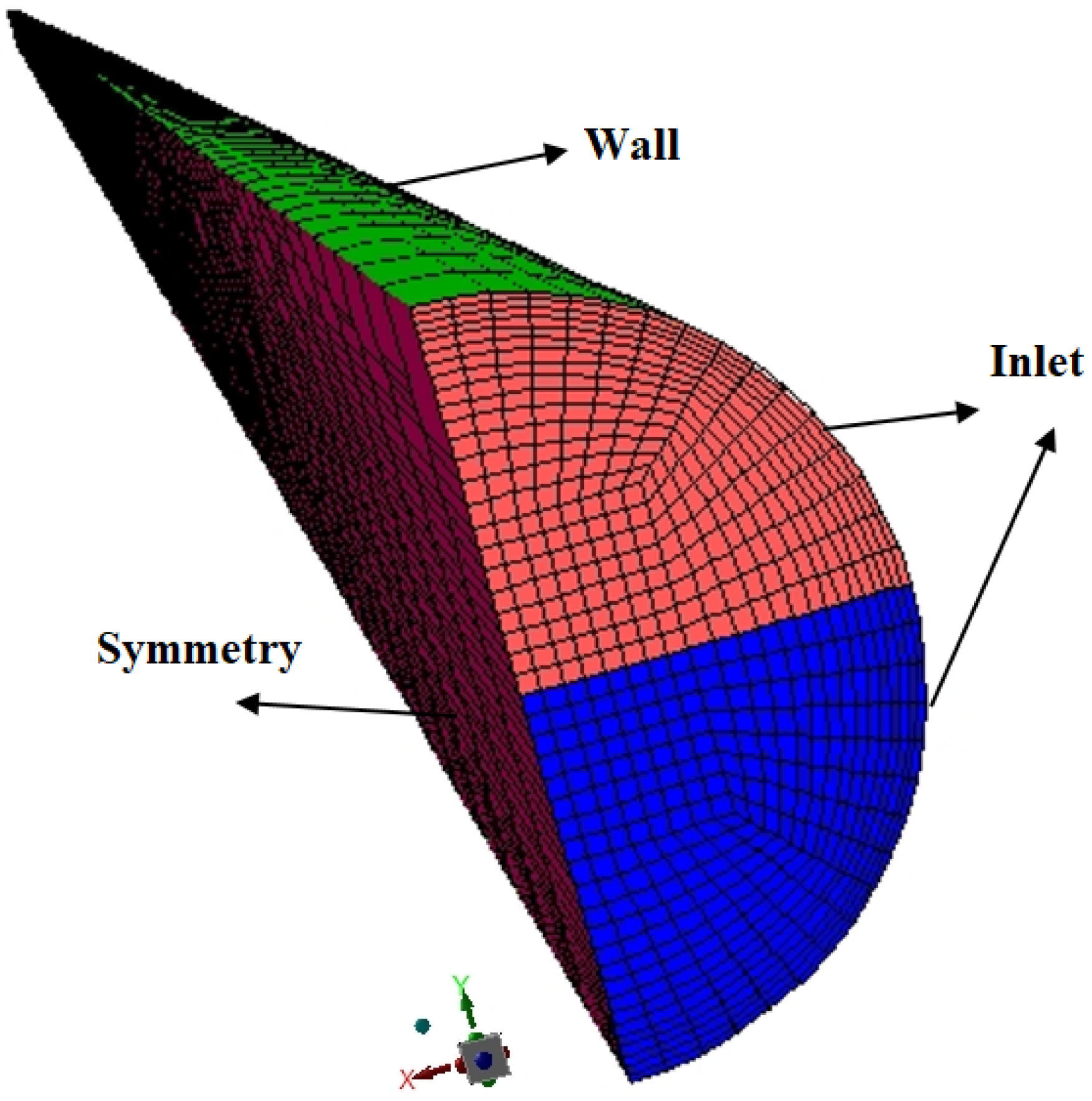
3. Geometry and Boundary Conditions

In the present study, the accuracy of the CFD model was assessed by using two sets of experimental data. The detailed information regarding the geometry of the pipes, as well as the fluid and flow properties are shown in

Table 1. The fluid properties and the geometrical conditions in the experiments.

Experimental Condition	Test 1 Angeli and Hewitt [52]	Test 2 Angeli and Hewitt [52]	Test 3 Elseth [72]	Test 4 Elseth [72]
Pipe diameter	2.43$\times {10}^{-2}$ m	2.43$\times {10}^{-2}$ m	5.6$\times {10}^{-2}$ m	5.63$\times {10}^{-2}$ m
Pipe length	9.7 m	9.7 m	15 m	15 m
Pipe roughness	7$\times {10}^{-7}$ m	7$\times {10}^{-7}$ m	1$\times {10}^{-6}$ m	1$\times {10}^{-6}$ m
Oil viscosity	1.6 mPa·s	1.6 mPa·s	1.64 mPa·s	1.64 mPa·s
Oil density	8.01$\times {10}^2$ Kg/m3	8.01$\times {10}^2$ Kg/m3	7.9$\times {10}^2$ Kg/m3	7.9$\times {10}^2$ Kg/m3
Flow velocity	1.25 m/s	1.7 m/s	2 m/s	1 m/s
Water cut	5$\times {10}^{-2}$	5$\times {10}^{-2}$	1$\times {10}^{-1}$	1$\times {10}^{-1}$
Interfacial tension	1.7$\times {10}^{-2}$ N/m	1.7$\times {10}^{-2}$ N/m	4.3$\times {10}^{-2}$ N/m	4.3$\times {10}^{-2}$ N/m

[62,82]. Numerical simulations were performed for two horizontal pipes with the internal diameter of 0.0563 m and 0.0243 m, respectively.

In the experiment carried out by Elseth [82], oil and water were introduced into the pipe from top and bottom, respectively. Although, in Angeli and Hewitt [62] the oil and water were mixed using a T-junction at the inlet. In order to satisfy the experimental conditions of Elseth [82], oil and water were introduced separately by assigning two separate velocity inlet boundary conditions. Similar to the experiment, the water cuts and the mixture velocities in the pipe were adjusted by regulating the velocity of each phase at the inlets. One velocity inlet, consisting a mixture of oil and water, was considered as an inlet for the experiment of Angeli and Hewitt [62]. The CFD model was initialized by assuming a single phase oil flow while the dispersed phase droplets entered to the physical domain from the corresponding inlets according to the experiment. Furthermore, the hydraulic diameter and turbulent intensity at the inlets were specified based on the pipe diameter and the fluid or flow properties. The turbulent intensity at the inlet was estimated as follows:

$$I=0.16R{e}^{\frac{-1}{8}}$$

(23)

A pressure outlet boundary condition was considered for the outlet boundary and the gauge pressure was considered zero, which is compatible with the separator pressure in the experiments.

A no-slip boundary condition was applied at the wall of the pipe. A symmetric boundary condition was adopted in the present study to reduce the computational. A grid sensitivity study was performed and a grid consist of 364,000 hexahedral cells was found to be suitable for model the experiments conducted by Elseth [82]. The same grid was scaled for modelling the experiment of Angeli and Hewitt [52]. GAMBIT 2.3.16 [83] was used to generate the geometry and the grid. Figure 1 shows the employed grid, as well as the boundary conditions in the present study.

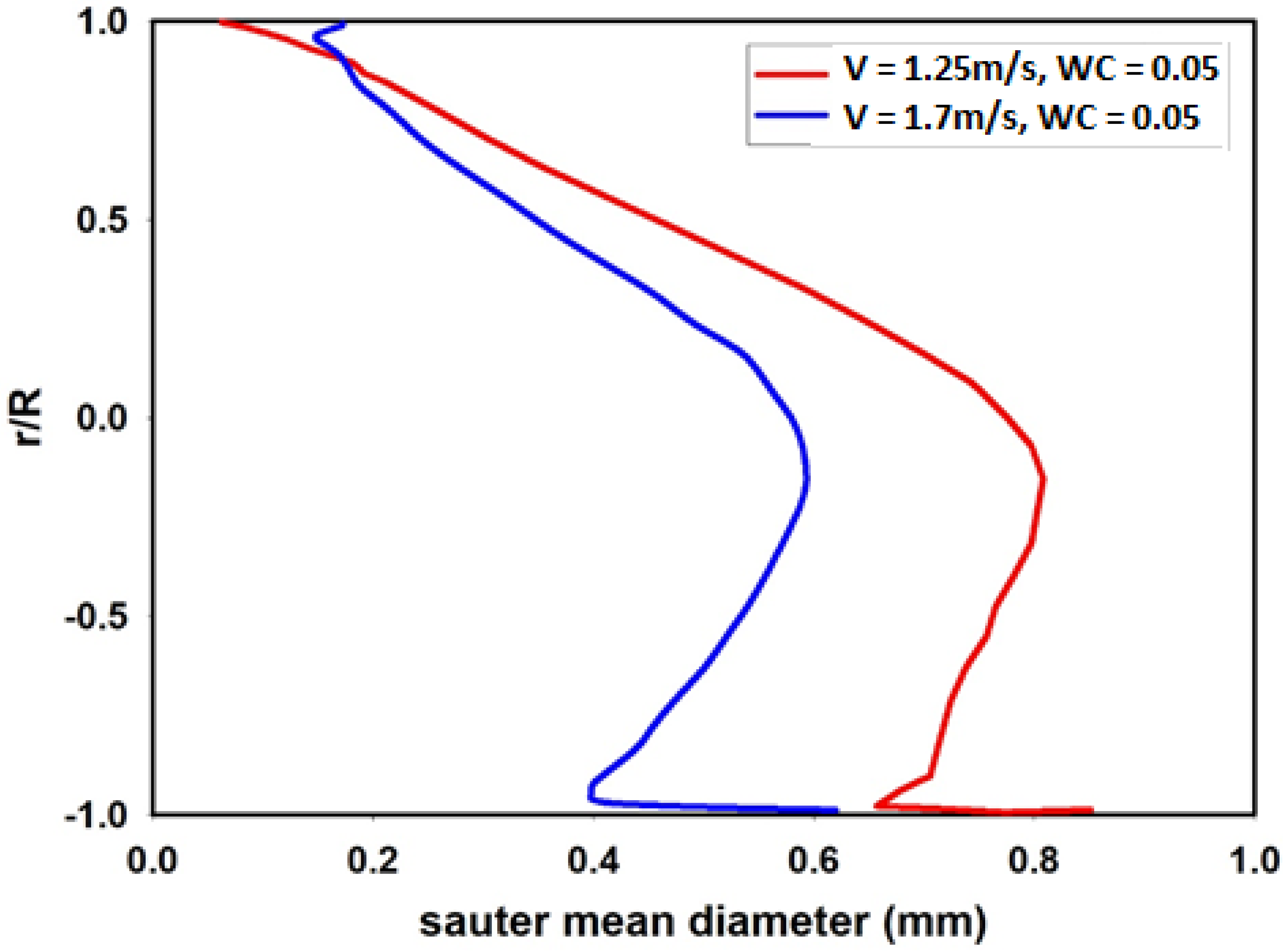
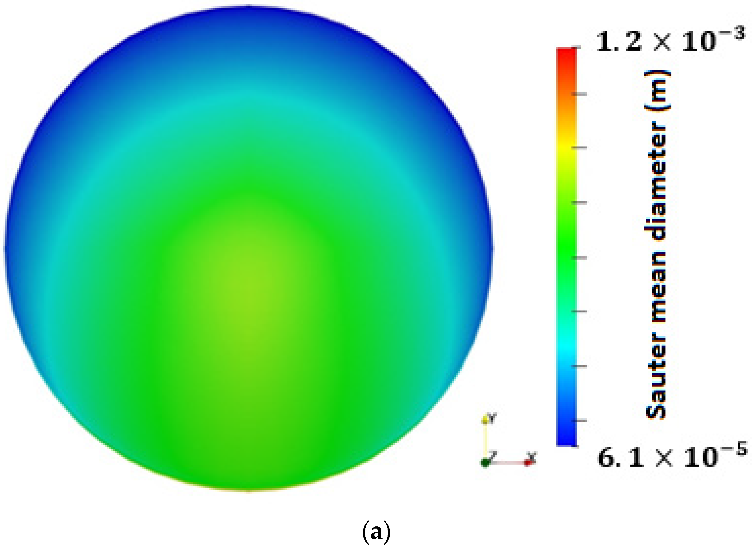
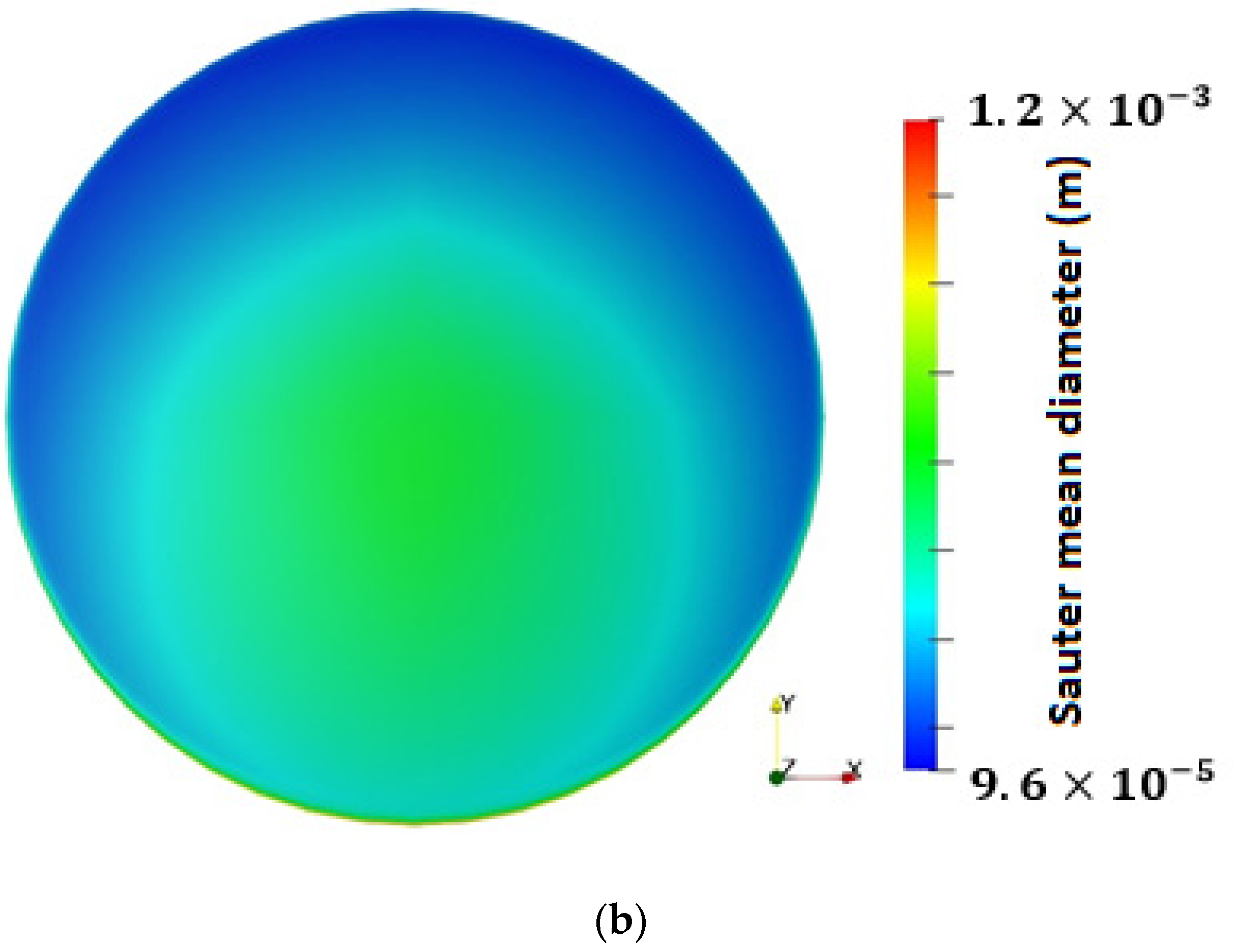
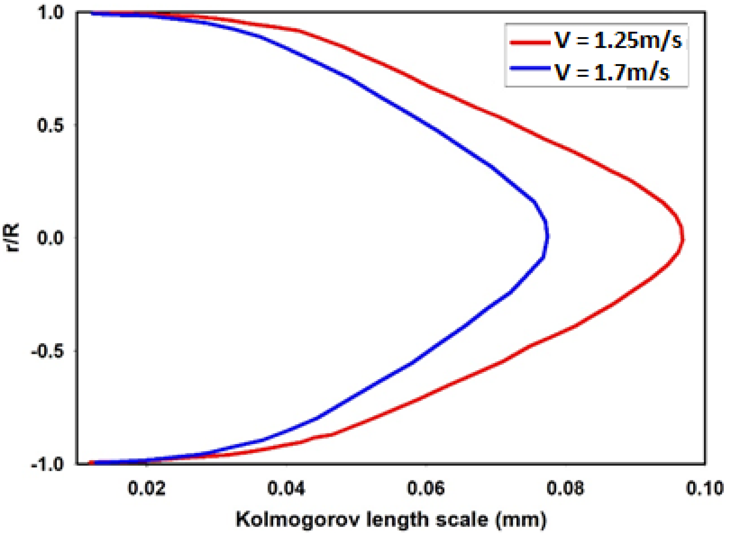
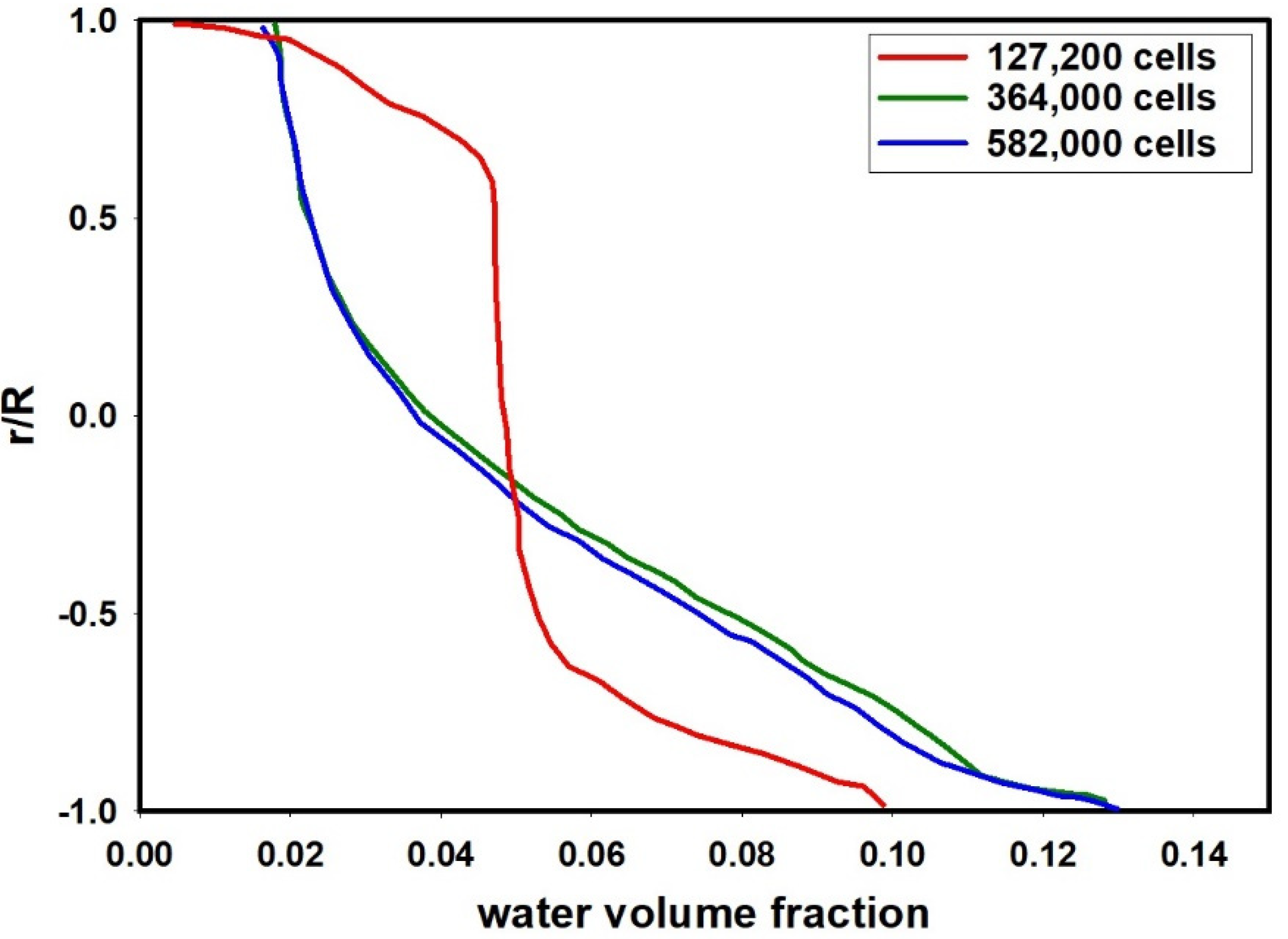
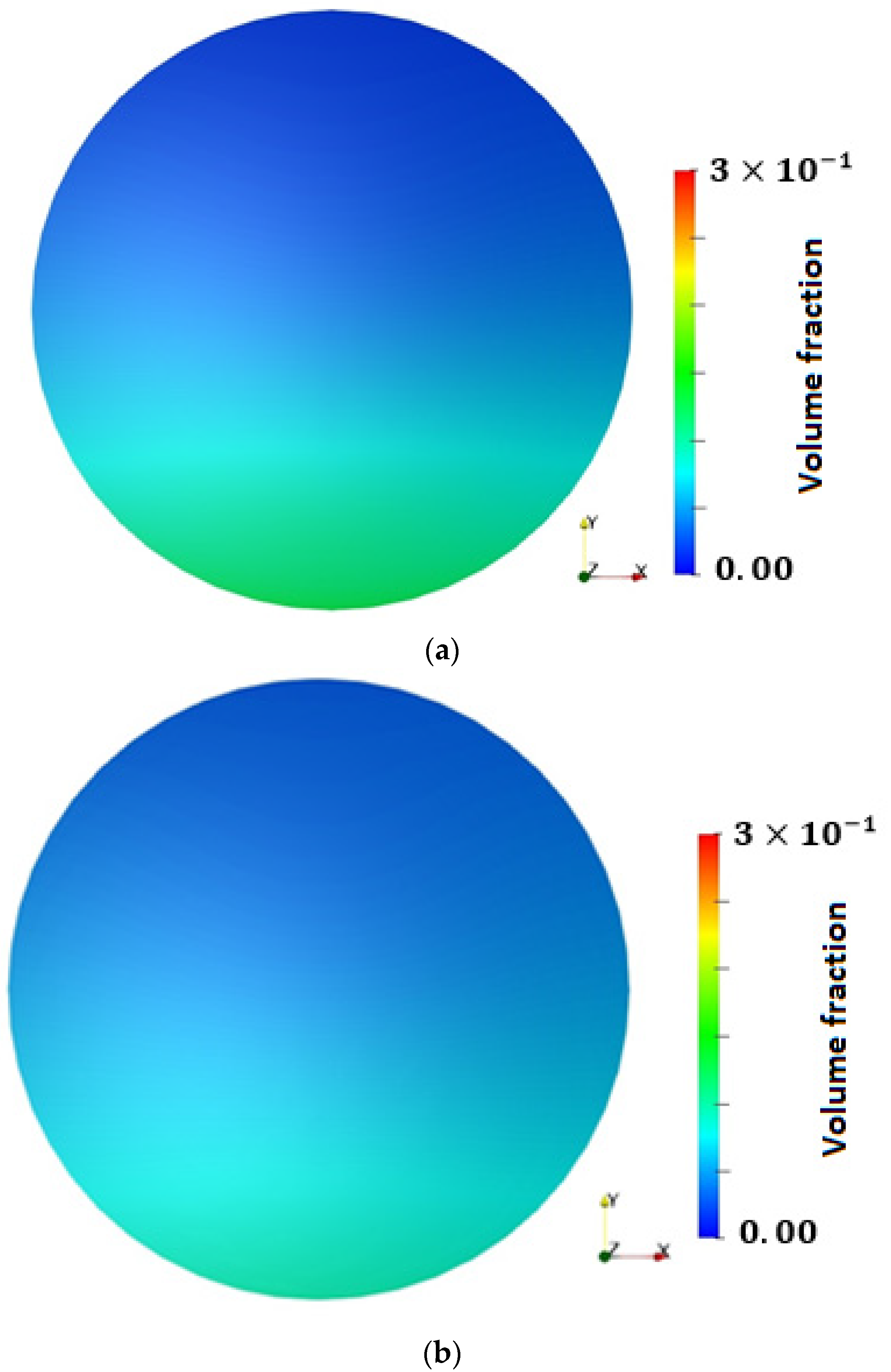
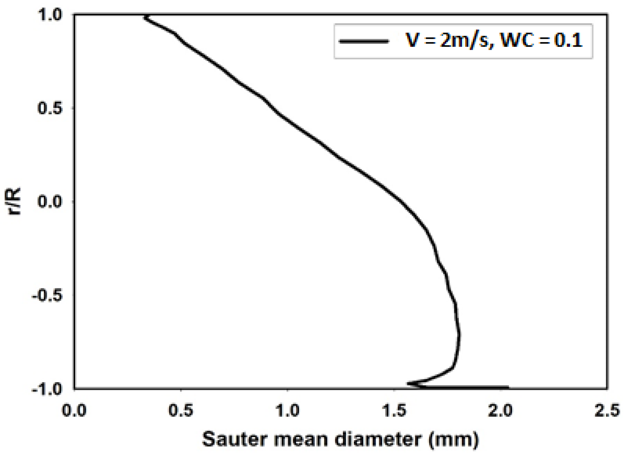
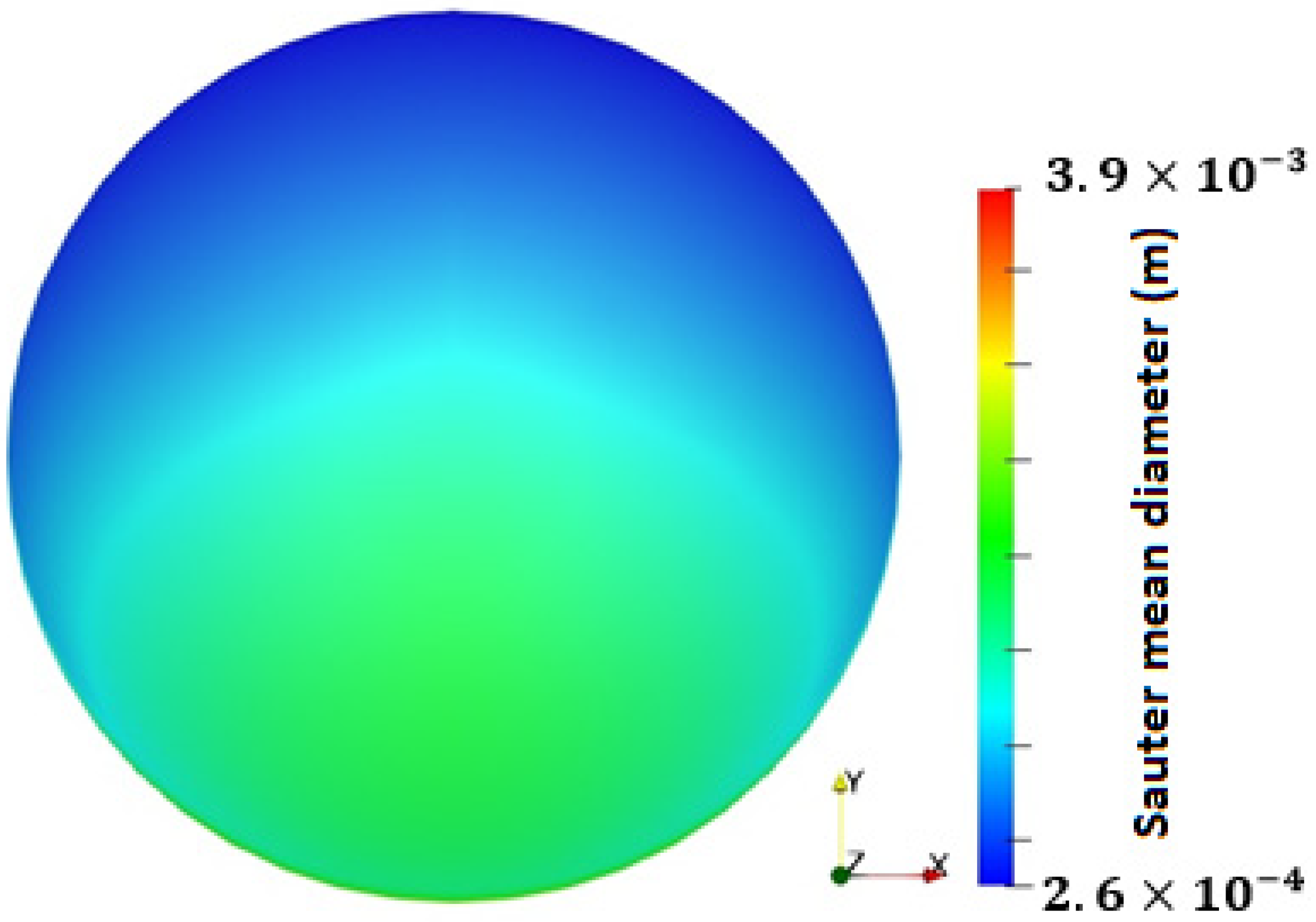
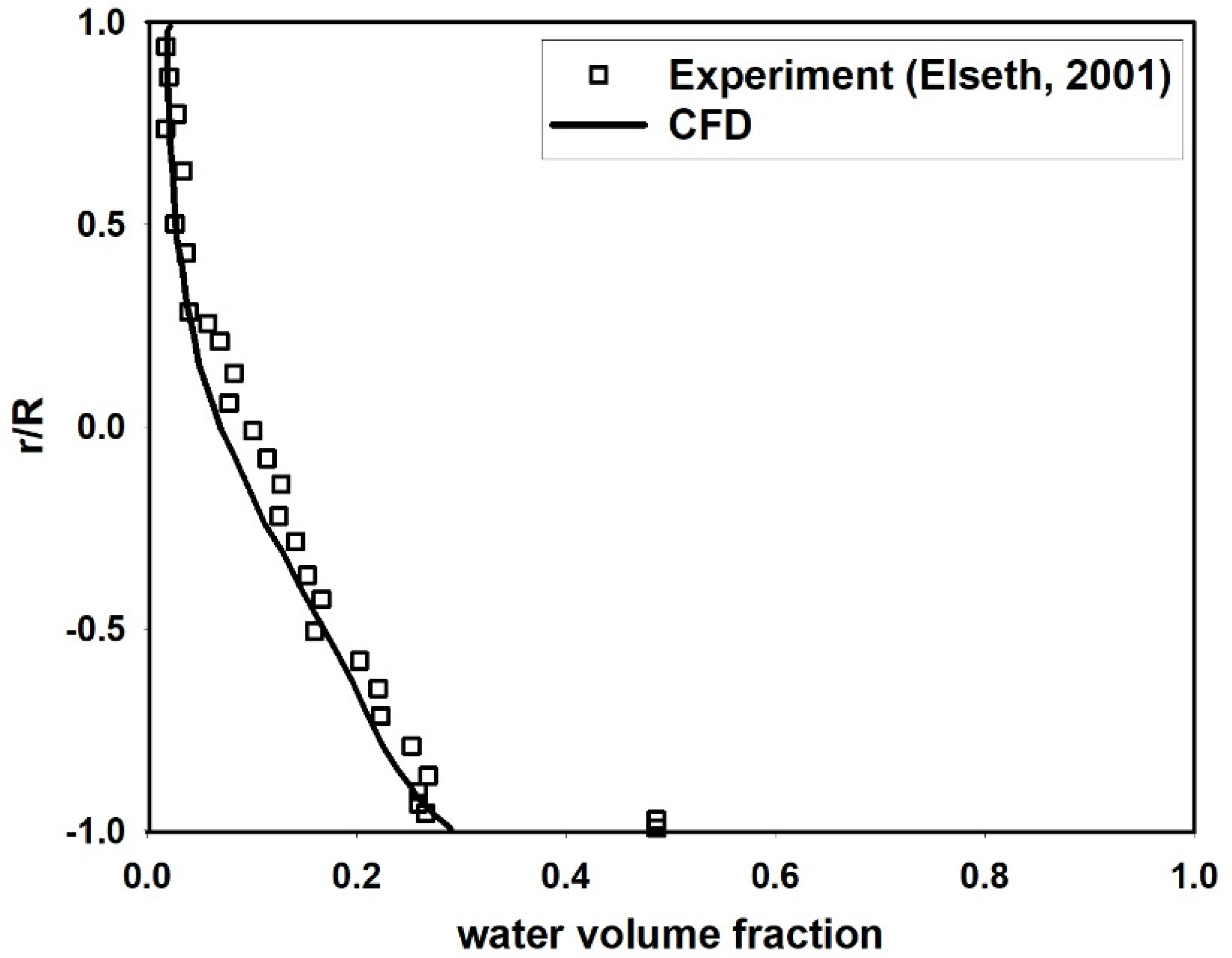
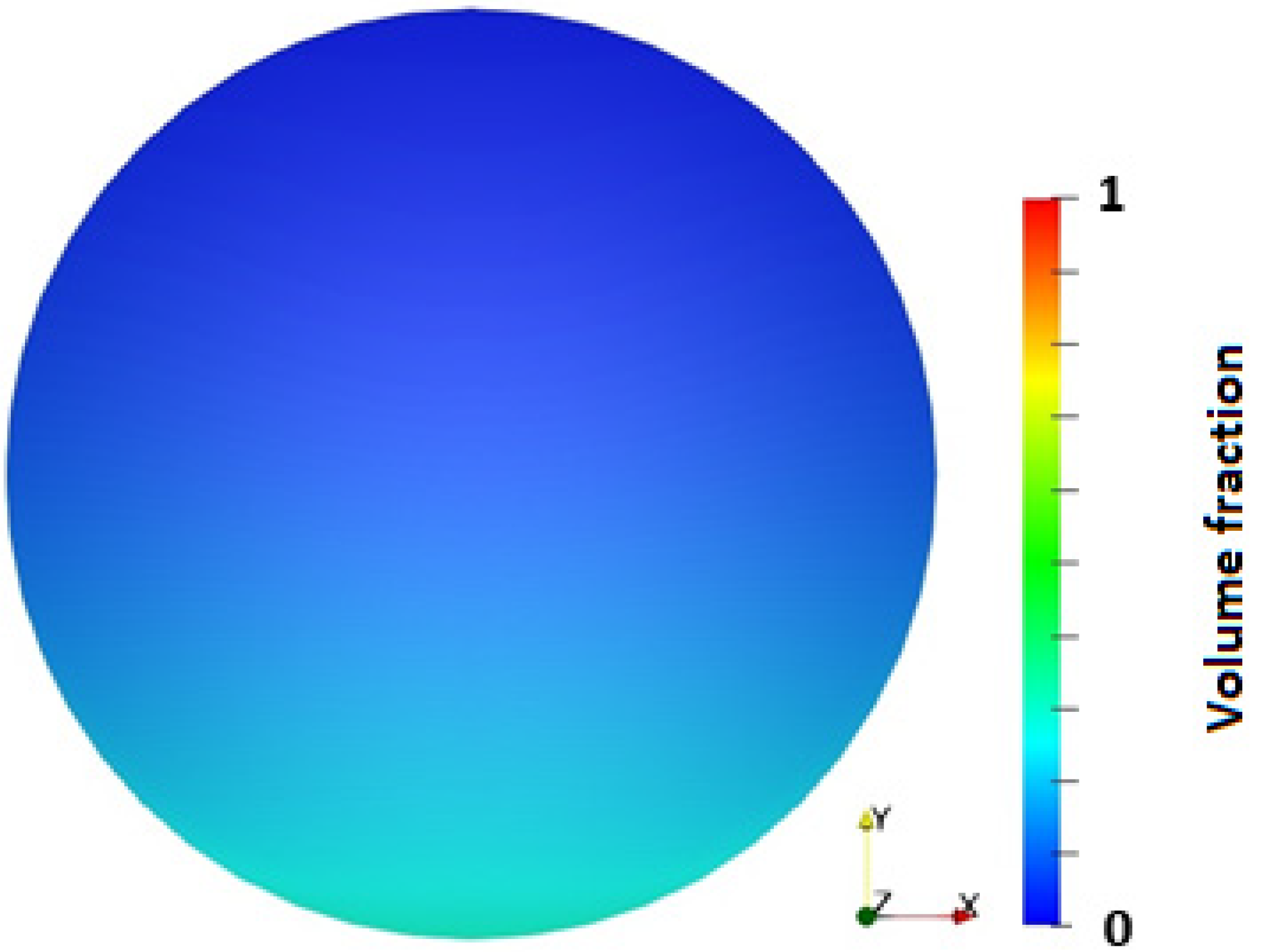
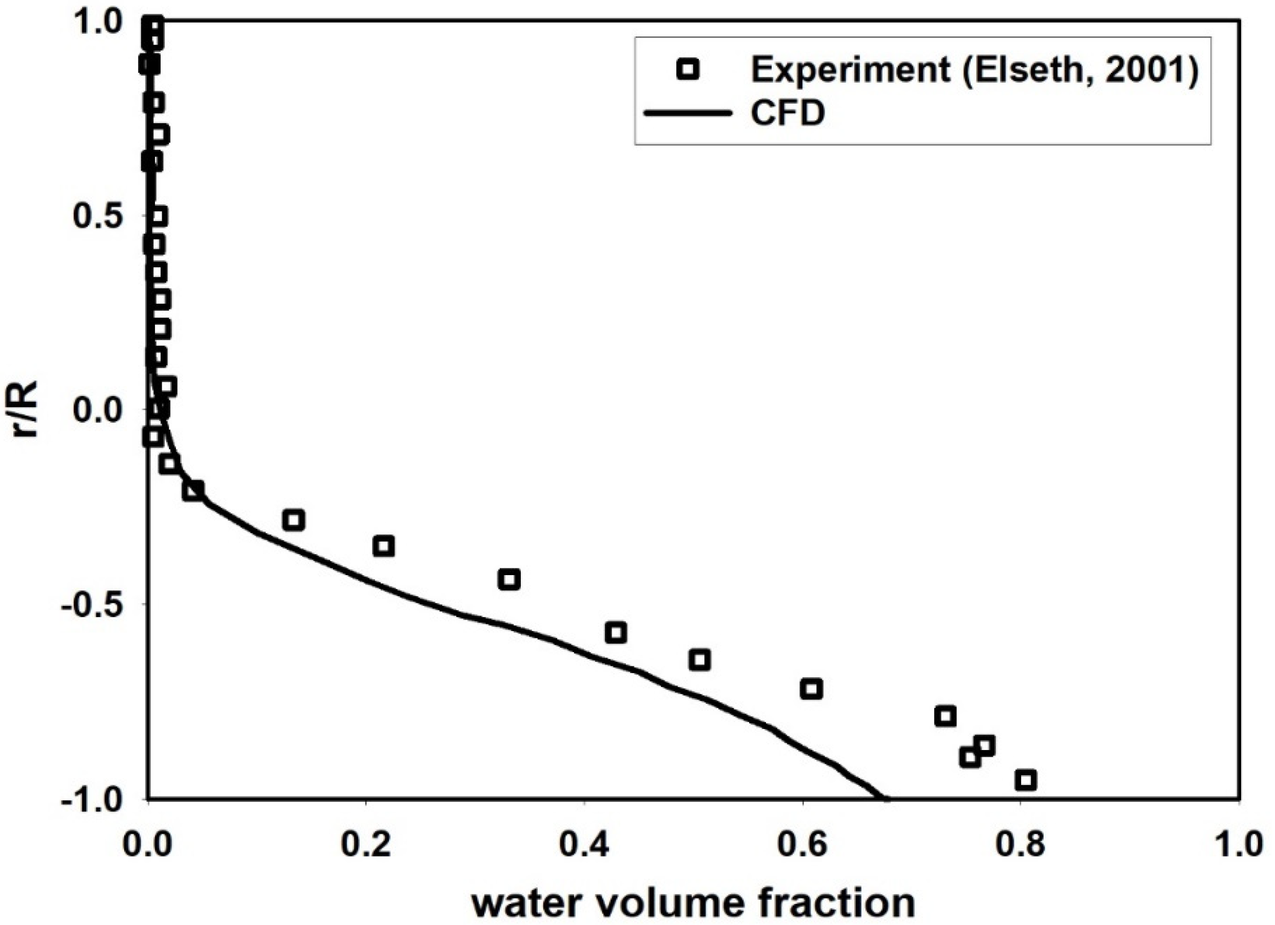
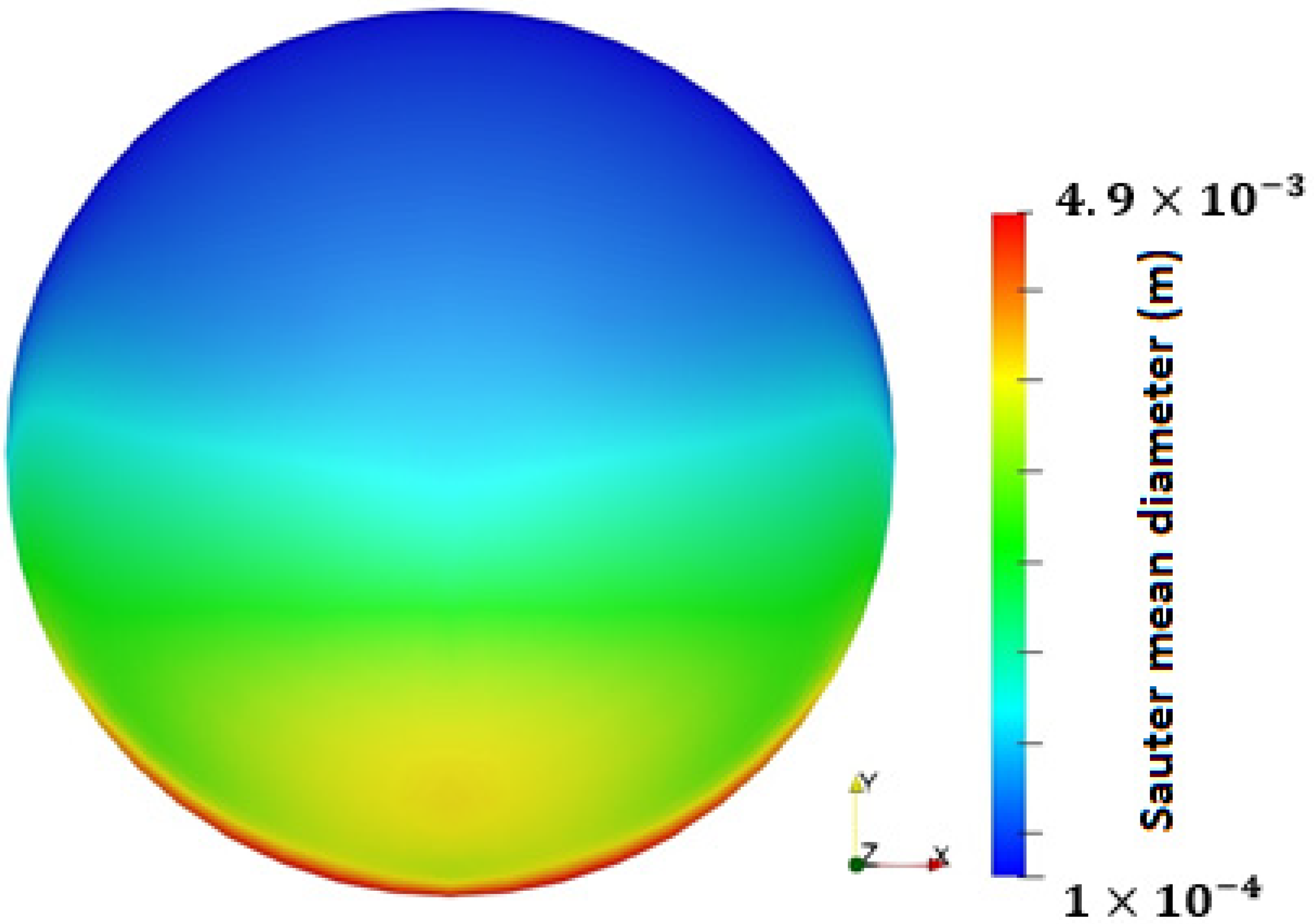
4. Results and Discussions

Numerical simulations were performed based on the described models in the previous section. Four experimental tests were used to evaluate the accuracy of the CFD model in estimating the Sauter mean diameter and water distribution. The capability of the CFD model in predicting the in-situ droplet size was judged by making a comparison with the experimental data of Angeli and Hewitt [62] corresponding to a dilute dispersion of water in oil flow. Furthermore, the experimental data of Elseth [82] was used to evaluate the accuracy of the CFD model in predicting the distribution of the volume fraction of the dispersed water droplets across the pipe section. The physical properties of the fluids and pipes specifications for all the tests can be found in Table 1.

As mentioned, test 1 and test 2 were chosen as a benchmark for assessing the accuracy of the droplet size predictions. The input water cut of both test 1 and test 2 were 0.05, while the flow velocities were 1.25 m/s and 1.7 m/s, respectively. The minimum and maximum droplet sizes were set to 5 × 10⁻⁵ m and 3.2 × 10⁻³ m, respectively. Furthermore, the specified range of droplet sizes in the population balance model was divided into 10 intervals or classes (bins). It should be mentioned that in the experiment the endoscope window was placed at the core of the pipe and the maximum depth of view was limited to 4.5 mm upward. Hence, the area weighted average of the predicted Sauter mean diameter by CFD model in this area was determined to compare with the experimental measurement data.

Table 2. The Sauter mean diameter as measured in the experiment and predicted by CFD model.

Experimental Condition	Sauter Mean Diameter 1.7 m/s	Sauter Mean Diameter 1.25 m/s
Measurement	0.35 mm	0.6mm
CFD-PBM	0.456 mm	0.665 mm

shows the Sauter mean diameter for test 1 and test 2 as measured in the experiments and predicted by the CFD model.

A comparison of the predicted and measured Sauter mean diameters using the present CFD model and the experiment indicates a reasonable accuracy of the CFD model. However, the CFD model slightly over predicted the Sauter mean diameter for both tests. Furthermore, the measurement of Sauter mean diameter at two different velocities suggests that an increase in the mixture velocity results in a decrease in the Sauter mean diameter. This trend is also observed in the predictions of the CFD model.

Figure 2 shows the vertical distribution of Sauter mean diameter in whole pipe cross section for test 1 and test 2 as predicted by the CFD model. According to this figure, regardless of the magnitude of the droplet size, the distribution of the droplet size across the pipe section is very similar for both tests. As shown in Figure 2, the Sauter mean diameter at the top of the pipe is very small. As we move downward, the Sauter mean diameter significantly increases until reaching its maximum value at slightly below the center of the pipe. However, by further moving downward a gradual decrease in the droplet size is observed, except in the region close to the bottom wall where the droplet size suddenly increases. This trend generally agrees well with the experimental observations since due to the higher turbulence dissipation rate the breakup rate near the wall region is the highest. The observed sudden increase in the droplet size in flow region adjacent to the bottom wall might be attributed to the low accuracy of the adopted turbulence model in this study, which is assuming the isotropic turbulence while the turbulence near the wall is clearly anisotropic. Furthermore, the high volume fraction of the dispersed phase at the bottom of the pipe may increase the probability of coalescence, thereby, increasing the droplet size. Figure 3 shows the contours of Sauter mean diameter at the pipe cross section as predicted by using the CFD model.

The application of the used breakup and coalescence models in this study is limited to the inertial subrange of turbulence. Furthermore, the model presented by Brauner [61] is an extension of Hinze [63] model, which is also based on the particle breakage in the inertial subrange. Hence, the size of the dispersed droplets should be larger than the size of the smallest eddies that are recognized as the Kolmogorov length scale. Figure 4 shows the Kolmogorov length scale across the pipe cross section, which indicates the size of the smallest eddies. A comparison of the size of the predicted Sauter mean diameter in Figure 2 and the smallest eddies in Figure 4 clearly reveals that the dispersed droplets are larger than the size of the smallest eddies, thereby, more prone to the turbulent inertial subrange. Hence, the influence of viscos breakage can be neglected.

Figure 5 depicts the vertical distribution of the dispersed water volume fraction from the developed CFD model in this work for test 1 and test 2 with the mixture velocities of 1.25 m/s and 1.7 m/s, respectively. As seen, a relatively homogeneous dispersion is predicted by the CFD model in which the water volume fraction increases as moving to the bottom of the pipe. This figure also reveals that for a constant input volume fraction of the dispersed phase an increase in the mixture velocity results in a more homogeneous dispersion. As mentioned earlier, the mesh sensitivity study was conducted to make sure that the obtained CFD results are independent of the mesh resolution. Figure 6 shows the distribution of water volume fraction across the pipe section for test 2 with the mixture velocity of 1.25 m/s and 5% water cut. As seen in this figure, by increasing the cell number beyond 364,000 the obtained numerical results would not change significantly. Figure 7 shows the contours of water volume fraction across the pipe section as obtained by the CFD model for test 1 and test 2.

Numerical simulations of dispersed water in oil flow were also conducted for two different tests (test 3 and test 4) with available in-situ dispersed phase distributions. The experimental data were taken from Elseth [82]. The operating conditions of test 3 and test 4 have been reported in Table 1. Figure 8 shows the vertical distribution of Sauter mean diameter for test 3, in which the mixture velocity and water cut are 2 m/s and 0.1, respectively. A similar distribution of Sauter mean diameter as observed in Figure 2 is perceived in this figure. The minimum and maximum droplet sizes of 1 × 10⁻⁴ m and 5.5 × 10⁻³ m were chosen to specify the range of the droplet size distribution in population balance model, which was divided into 10 intervals or classes (bins). As seen, the Sauter mean diameter at the top of the pipe is very small and as we move downward it significantly increases, following a decrease after reaching its maximum value. However, similar to the observed phenomenon in Figure 2, a sudden increase in the droplet size is observed closed to the wall. Due to the limited experimental data for the in-situ distribution of the droplet size, the accuracy of the predicted Sauter mean diameter cannot be assessed. Figure 9 shows the contours of Sauter mean diameter across the pipe section by using the CFD model.

Figure 10 illustrates a comparison of the vertical distribution of water volume fraction in pipe cross section as obtained by the combined CFD-PBM model and the experimental measurement using a gamma densitometer. According to this figure, the CFD model could reasonably predict the water distribution across the pipe section. A small deviation observed at the bottom of the pipe could be attributed to the deficiency of the adopted closure laws for turbulent dispersion or the lift forces. The present study employed the turbulent dispersion force suggested by Lopez de Bertodano [72] in which the turbulent dispersion coefficient was a constant. Using a constant dispersion coefficient throughout the computational domain is a common practice in most of the studies regarding the CFD modelling of the dispersed flows [84,85]. However, from the physical point of view the turbulent dispersion coefficient is a function of the Stokes number which is defined as the ratio of a response time of the dispersed particles to the eddies of the continuous phase [71,72]. Hence, using a variable turbulent dispersion coefficient could potentially enhance the accuracy of the CFD solution. Apart from that, using other turbulent dispersion force models such as the model proposed by Burns et al. [86] may result in better predictions.

Figure 11 shows the contours of water volume fraction distribution across the pipe section as obtained by the CFD model for test 3.

Figure 12 shows the contours of the in-situ water volume fraction distribution for test 4 as obtained by the CFD-PBM model. The mixture velocity and water cut for this test are 1 m/s and 0.1, respectively. In the CFD model, the minimum and maximum droplet sizes of 1 × 10⁻⁴ m and 6.4 × 10⁻³ m were chosen to specify the range of the droplet size distribution. Furthermore, the droplet size distribution range was divided into 11 classes.

Figure 13 depicts a comparison of the predicted vertical distribution of water volume fraction by using CFD model and the experimental measurement using gamma densitometer. According to this figure the CFD model could reasonably predict the distribution of dispersed water phase across the pipe section. As seen in this figure, the experimental measurement, as well as the CFD model revealed the occurrence of a dense water dispersion in oil at the bottom of the pipe. The models developed for the lift force can be applicable for relatively dilute systems where a dense packing of the dispersed phase does not occur [80,87]. Hence, using such models for dispersed phase volume fractions higher than 0.5 is questionable and likely to give physically misleading results. Furthermore, when the volume fraction of the dispersed phase increases, the lift coefficient tends to approach zero [87,88]. Apart from these, the influence of the lift force for regions close to the center of the pipe is negligible. Thus, the influence of lift force has been neglected for this case as the droplet volume fraction at the bottom of the pipe exceeds 0.5.

Figure 14 shows the vertical distribution of Sauter mean diameter for test 4. It is observed that the distribution of Sauter mean diameter is quite similar to the predicted distribution for test 3. However, due to the lower mixture velocity the probability of breakup decreases, while the coalescence probability increases. Hence, the average Sauter mean diameter for test 4 is larger than that for test 3. Figure 15 shows the contours of the predicted Sauter mean diameter for test 4.

5. Conclusions

A three-dimensional numerical modelling of turbulent dispersed water in oil flow pattern through a horizontal pipe was carried out in the present study. Numerical modelling was conducted using a two-fluid Eulerian approach. Four interfacial forces namely, the drag, virtual mass, lift and turbulent dispersion were considered to close the two-fluid model. The standard K-epsilon model was employed to model the turbulent effects. Furthermore, the droplet size distribution was modelled by using a population balance model based on the method of class in which the breakup and coalescence events were modelled using Lehr and Luo models, respectively.

A comparison of the predicted Sauter mean diameter by using the CFD model with the corresponding experimental data indicates that a combination of the Luo coalescence model and the Lehr breakup model can reasonably predict the Sauther mean diameter.

Numerical results of the in-situ water fraction distributions were also compared with the available experimental data. According to the obtained CFD results, a combination of the adopted interfacial force models and the predicted Sauter mean diameter using the population balance model resulted in a reasonable prediction of the dispersed water distribution.

The obtained results of the present study revealed the capability of the employed CFD model for predicting the main features of complex dispersed oil-water flows in pipeline. However, the adopted closure laws for the interfacial forces require further study and calibration. Moreover, a comparative study of different breakup and coalescence models is essential to identify the most appropriate kernels for modelling the developing dispersed oil–water flows.

References

1. Angeli, P.; Hewitt, G.F. Flow structure in horizontal oil–water flow. Int. J. Multiph. Flow 2000, 26, 1117–1140. [Google Scholar] [CrossRef]
2. Ahmed, S.A.; John, B. Liquid–Liquid horizontal pipe flow–A review. J. Pet. Sci. Eng. 2018, 168, 426–447. [Google Scholar] [CrossRef]
3. Xu, X.X. Study on oil-water two phase floe in pipelines. J. Pet. Sci. Eng. 2007, 59, 43–58. [Google Scholar] [CrossRef]
4. Lovick, J.; Angeli, P. Experimental studies on the dual continuous flow pattern in oil–water flows. Int. J. Multiph. Flow 2004, 30, 139–157. [Google Scholar] [CrossRef]
5. Kumara, W.A.S.; Halvorsen, B.M.; Melaaen, M.C. Pressure drop, flow pattern and local water volume fraction measurements of oil–water flow in pipes. Meas. Sci. Technol. 2009, 20, 114004. [Google Scholar] [CrossRef]
6. Yusuf, N.; Al-Wahaibi, Y.; Al-Wahaibi, T.; Al-Ajmi, A.; Olawale, A.S.; Mohammed, I.A. Effect of oil viscosity on the flow structure and pressure gradient in horizontal oil–water flow. Chem. Eng. Res. Des. 2012, 90, 1019–1030. [Google Scholar] [CrossRef]
7. Ismail, A.S.I.; Ismail, I.; Zoveidavianpoor, M.; Mohsin, R.; Piroozian, A.; Misnan, M.S.; Sariman, M.Z. Review of oil–water through pipes. Flow Meas. Instrum. 2015, 45, 357–374. [Google Scholar] [CrossRef]
8. Prieto, L.; Muñoz, F.; Pereyra, E.; Ratkovich, N. Pressure gradient correlations analysis for liquid-liquid flow in horizontal pipes. J. Pet. Sci. Eng. 2018, 169, 683–704. [Google Scholar] [CrossRef]
9. Boxall, J.A.; Koh, C.A.; Sloan, E.D.; Sum, A.K.; Wu, D.T. Droplet size scaling of water-in-oil emulsions under turbulent flow. Langmuir 2011, 28, 104–110. [Google Scholar] [CrossRef] [PubMed]
10. Zhang, H.; Lan, H.Q. A review of internal corrosion mechanism and experimental study for pipelines based on multiphase flow. Corros. Rev. 2017, 35, 425–444. [Google Scholar] [CrossRef]
11. Apte, M.S.; Matzain, A.; Zhang, H.Q.; Volk, M.; Brill, J.P.; Creek, J.L. Investigation of paraffin deposition during multiphase flow in pipelines and wellbores—Part 2: Modeling. J. Energy Resour. Technol. 2001, 123, 150–157. [Google Scholar] [CrossRef]
12. Sarica, C.; Panacharoensawad, E. Review of paraffin deposition research under multiphase flow conditions. Energy Fuels 2012, 26, 3968–3978. [Google Scholar] [CrossRef]
13. Akhfash, M.; Aman, Z.M.; Ahn, S.Y.; Johns, M.L.; May, E.F. Gas hydrate plug formation in partially-dispersed water–oil systems. Chem. Eng. Sci. 2016, 140, 337–347. [Google Scholar] [CrossRef]
14. Sohn, Y.H.; Kim, J.; Shin, K.; Chang, D.; Seo, Y.; Aman, Z.M.; May, E.F. Hydrate plug formation risk with varying water cut and inhibitor concentrations. Chem. Eng. Sci. 2015, 126, 711–718. [Google Scholar] [CrossRef]
15. Danielson, T.J. Transient multiphase flow: Past, present, and future with flow assurance perspective. Energy Fuels 2012, 26, 4137–4144. [Google Scholar] [CrossRef]
16. Paolinelli, L.D.; Rashedi, A.; Yao, J.; Singer, M. Study of water wetting and water layer thickness in oil-water flow in horizontal pipes with different wettability. Chem. Eng. Sci. 2018, 183, 200–214. [Google Scholar] [CrossRef]
17. Gao, H.; Gu, H.Y.; Guo, L.J. Numerical study of stratified oil–water two-phase turbulent flow in a horizontal tube. Int. J. Heat Mass Transf. 2003, 46, 749–754. [Google Scholar] [CrossRef]
18. Al-Yaari, M.A.; Abu-Sharkh, B.F. CFD prediction of stratified oil-water flow in a horizontal pipe. Asian Trans. Eng. 2011, 1, 68–75. [Google Scholar]
19. Shi, J.; Gourma, M.; Yeung, H. CFD simulation of horizontal oil-water flow with matched density and medium viscosity ratio in different flow regimes. J. Pet. Sci. Eng. 2007, 151, 373–383. [Google Scholar] [CrossRef] [Green Version]
20. Beerens, J.C.; Ooms, G.; Pourquie, M.J.; Westerweel, J. A comparison between numerical predictions and theoretical and experimental results for laminar core-annular flow. AIChE J. 2014, 60, 3046–3056. [Google Scholar] [CrossRef]
21. Desamala, A.B.; Vijayan, V.; Dasari, A.; Dasmahapatra, A.K.; Mandal, T.K. Prediction of oil-water flow patterns, radial distribution of volume fraction, pressure and velocity during separated flows in horizontal pipe. J. Hydrodyn. Ser. B 2016, 28, 658–668. [Google Scholar] [CrossRef]
22. Kaushik, V.V.R.; Ghosh, S.; Das, G.; Das, P.K. CFD simulation of core annular flow through sudden contraction and expansion. J. Pet. Sci. Eng. 2012, 86, 153–164. [Google Scholar] [CrossRef]
23. Ghosh, S.; Das, G.; Das, P.K. Simulation of core annular downflow through CFD—A comprehensive study. Chem. Eng. Process. Process. Intensif. 2010, 49, 1222–1228. [Google Scholar] [CrossRef]
24. Dehkordi, P.B.; Colombo, L.P.M.; Guilizzoni, M.; Sotgia, G. CFD simulation with experimental validation of oil-water core-annular flows through Venturi and Nozzle flow meters. J. Pet. Sci. Eng. 2017, 149, 540–552. [Google Scholar] [CrossRef]
25. Dehkordi, P.B.; Azdarpour, A.; Mohammadian, E. The hydrodynamic behavior of high viscous oil-water flow through horizontal pipe undergoing sudden expansion—CFD study and experimental validation. Chem. Eng. Res. Des. 2018, 139, 144–161. [Google Scholar] [CrossRef]
26. Xu, G.; Cai, L.; Ullmann, A.; Brauner, N. Experiments and simulation of water displacement from lower sections of oil pipelines. J. Pet. Sci. Eng. 2016, 147, 829–842. [Google Scholar] [CrossRef]
27. Song, X.; Yang, Y.; Zhang, T.; Xiong, K.; Wang, Z. Studies on water carrying of diesel oil in upward inclined pipes with different inclination angle. J. Pet. Sci. Eng. 2017, 157, 780–792. [Google Scholar] [CrossRef]
28. Magnini, M.; Ullmann, A.; Brauner, N.; Thome, J.R. Numerical study of water displacement from the elbow of an inclined oil pipeline. J. Pet. Sci. Eng. 2018, 166, 1000–1017. [Google Scholar] [CrossRef]
29. Zhang, H.; Lan, H.Q.; Lin, N. A numerical simulation of water distribution associated with internal corrosion induced by water wetting in upward inclined oil pipes. J. Pet. Sci. Eng. 2019, 173, 351–361. [Google Scholar] [CrossRef]
30. Liu, X.; Gong, C.; Zhang, L.; Jin, H.; Wang, C. Numerical study of the hydrodynamic parameters influencing internal corrosion in pipelines for different elbow flow configurations. Eng. Appl. Comput. Fluid Mech. 2020, 14, 122–135. [Google Scholar] [CrossRef] [Green Version]
31. Hirt, C.W.; Nichols, B.D. Volume of fluid (VOF) method for the dynamics of free boundaries. J. Comput. Phys. 1981, 39, 201–225. [Google Scholar] [CrossRef]
32. Osher, S.; Sethian, J.A. Fronts propagating with curvature-dependent speed: Algorithms based on Hamilton-Jacobi formulations. J. Comput. Phys. 1988, 79, 12–49. [Google Scholar] [CrossRef] [Green Version]
33. Unverdi, S.O.; Tryggvason, G. A front-tracking method for viscous, incompressible, multi-fluid flows. J. Comput. Phys. 1992, 100, 25–37. [Google Scholar] [CrossRef] [Green Version]
34. Azadbakhti, R.; Pourfattah, F.; Ahmadi, A.; Akbari, O.A.; Toghraie, D. Eulerian–Eulerian multi-phase RPI modeling of turbulent forced convective of boiling flow inside the tube with porous medium. Int. J. Numer. Methods Heat Fluid Flow 2019. [Google Scholar] [CrossRef]
35. Barnoon, P.; Toghraie, D.; Dehkordi, R.B.; Abed, H. MHD mixed convection and entropy generation in a lid-driven cavity with rotating cylinders filled by a nanofluid using two phase mixture model. J. Magn. Magn. Mater. 2019, 483, 224–248. [Google Scholar] [CrossRef]
36. Li, Z.; Barnoon, P.; Toghraie, D.; Dehkordi, R.B.; Afrand, M. Mixed convection of non-Newtonian nanofluid in an H-shaped cavity with cooler and heater cylinders filled by a porous material: Two phase approach. Adv. Powder Technol. 2019, 30, 2666–2685. [Google Scholar] [CrossRef]
37. Barnoon, P.; Toghraie, D.; Dehkordi, R.B.; Afrand, M. Two phase natural convection and thermal radiation of Non-Newtonian nanofluid in a porous cavity considering inclined cavity and size of inside cylinders. Int. Commun. Heat Mass Transf. 2019, 108, 104285. [Google Scholar] [CrossRef]
38. Barnoon, P.; Toghraie, D.; Eslami, F.; Mehmandoust, B. Entropy generation analysis of different nanofluid flows in the space between two concentric horizontal pipes in the presence of magnetic field: Single-phase and two-phase approaches. Comput. Math. Appl. 2019, 77, 662–692. [Google Scholar] [CrossRef]
39. Mostafazadeh, A.; Toghraie, D.; Mashayekhi, R.; Akbari, O.A. Effect of radiation on laminar natural convection of nanofluid in a vertical channel with single-and two-phase approaches. J. Therm. Anal. Calorim. 2019, 138, 779–794. [Google Scholar] [CrossRef]
40. Toghraie, D.; Mashayekhi, R.; Arasteh, H.; Sheykhi, S.; Niknejadi, M.; Chamkha, A.J. Two-phase investigation of water-Al2O3 nanofluid in a micro concentric annulus under non-uniform heat flux boundary conditions. Int. J. Numer. Methods Heat Fluid Flow 2019. [Google Scholar] [CrossRef]
41. Varzaneh, A.A.; Toghraie, D.; Karimipour, A. Comprehensive simulation of nanofluid flow and heat transfer in straight ribbed microtube using single-phase and two-phase models for choosing the best conditions. J. Therm. Anal. Calorim. 2020, 139, 701–720. [Google Scholar] [CrossRef]
42. Burlutskiy, E.; Turangan, C.K. A computational fluid dynamics study on oil-in-water dispersion in vertical pipe flows. Chem. Eng. Res. Des. 2015, 93, 48–54. [Google Scholar] [CrossRef]
43. Burlutskii, E. CFD study of oil-in-water two-phase flow in horizontal and vertical pipes. J. Pet. Sci. Eng. 2018, 162, 524–531. [Google Scholar] [CrossRef]
44. Pouraria, H.; Seo, J.K.; Paik, J.K. Numerical study of erosion in critical components of subsea pipeline: Tees vs. bends. Ships Offshore Struct. 2017, 12, 233–243. [Google Scholar] [CrossRef]
45. Voulgaropoulos, V.; Jamshidi, R.; Mazzei, L.; Angeli, P. Experimental and numerical studies on the flow characteristics and separation properties of dispersed liquid-liquid flows. Phys. Fluids 2019, 31, 073304. [Google Scholar] [CrossRef] [Green Version]
46. Santos, D.S.; Faia, P.M.; Garcia, F.A.P.; Rasteiro, M.G. Experimental and simulated studies of oil/water fully dispersed flow in a horizontal pipe. J. Fluids Eng. 2019, 141. [Google Scholar] [CrossRef]
47. Stachnik, M.; Jakubowski, M. Multiphase model of flow and separation phases in a whirlpool: Advanced simulation and phenomena visualization approach. J. Food Eng. 2020, 274, 109846. [Google Scholar] [CrossRef]
48. Morgan, R.G.; Markides, C.N.; Hale, C.P.; Hewitt, G.F. Horizontal liquid–liquid flow characteristics at low superficial velocities using laser-induced fluorescence. Int. J. Multiph. Flow 2012, 43, 101–117. [Google Scholar] [CrossRef]
49. Schümann, H.; Tutkun, M.; Nydal, O.J. Experimental study of dispersed oil-water flow in a horizontal pipe with enhanced inlet mixing, Part 2: In-situ droplet measurements. J. Pet. Sci. Eng. 2016, 145, 753–762. [Google Scholar] [CrossRef] [Green Version]
50. Voulgaropoulos, V.; Angeli, P. Optical measurements in evolving dispersed pipe flows. Exp. Fluids 2017, 58, 170. [Google Scholar] [CrossRef] [Green Version]
51. Voulgaropoulos, V. Dynamics of Spatially Evolving Dispersed Flows. Ph.D. Thesis, University College London, London, UK, 2018. [Google Scholar]
52. Parvini, M.; Dabir, B.; Mohtashami, S.A. Numerical simulation of oil dispersions in vertical pipe flow. J. Jpn. Pet. Inst. 2010, 53, 42–54. [Google Scholar] [CrossRef]
53. Hamad, F.A.; He, S.; Khan, M.K.; Bruun, H.H. Development of kerosene–water two-phase up-flow in a vertical pipe downstream of A 90° bend. Can. J. Chem. Eng. 2013, 91, 354–367. [Google Scholar] [CrossRef]
54. Walvekar, R.G.; Choong, T.S.; Hussain, S.A.; Khalid, M.; Chuah, T.G. Numerical study of dispersed oil–water turbulent flow in horizontal tube. J. Pet. Sci. Eng. 2009, 65, 123–128. [Google Scholar] [CrossRef]
55. Torres-Monzón, C.F. Modeling of Oil-Water Flow in Horizontal and near Horizontal Pipes. Ph.D. Thesis, The University of Tulsa, Tulsa, OK, USA, 2006. [Google Scholar]
56. Pouraria, H.; Paik, J.K.; Seo, J.K. Modeling of oil-water flow in horizontal pipeline using CFD technique. In Proceedings of the ASME 2013 32nd International Conference on Ocean, Offshore and Arctic Engineering, Nantes, France, 9–14 June 2013; American Society of Mechanical Engineers: New York, NY, USA, 2013. [Google Scholar]
57. Pouraria, H.; Seo, J.K.; Paik, J.K. A numerical study on water wetting associated with the internal corrosion of oil pipelines. Ocean. Eng. 2016, 122, 105–117. [Google Scholar] [CrossRef]
58. Pouraria, H.; Seo, J.K.; Paik, J.K. Numerical modelling of two-phase oil–water flow patterns in a subsea pipeline. Ocean. Eng. 2016, 115, 135–148. [Google Scholar] [CrossRef]
59. Jiang, F.; Wang, Y.; Ou, J.; Chen, C. Numerical Simulation of Oil-Water Core Annular Flow in a U-Bend Based on the Eulerian Model. Chem. Eng. Technol. 2014, 37, 659–666. [Google Scholar] [CrossRef]
60. Darihaki, F.; Shirazi, S.A.; Feng, Q. A Transient Approach for Estimating Concentration of Water Droplets in Oil and Corrosion Assessment in the Oil and Gas Industry. In Proceedings of the Fluids Engineering Division Summer Meeting. American Society of Mechanical Engineers, San Francisco, CA, USA, 28 July–1 August 2019; Volume 59087, p. V005T05A077. [Google Scholar]
61. Brauner, N. The prediction of dispersed flows boundaries in liquid–liquid and gas–liquid systems. Int. J. Multiph. Flow 2001, 27, 885–910. [Google Scholar] [CrossRef]
62. Angeli, P.; Hewitt, G.F. Drop Size Distributions in Horizontal Oil-water Dispersed Flows, Dispersed Flows. Int. J. Multiph. Flow 2000, 27, 885–910. [Google Scholar]
63. Hinze, J.O. Fundamentals of the hydrodynamic mechanism of splitting in dispersion processes. AIChE J. 1955, 1, 289–295. [Google Scholar] [CrossRef]
64. Voulgaropoulos, V.; Zhai, L.; Ioannou, K.; Angeli, P. Evolution of unstable liquid-liquid dispersions in horizontal pipes. In Proceedings of the 10th North American Conference on Multiphase Technology, Banff, AB, Canada, 8–10 June 2016; BHR Group: Wharley End, UK, 2016. [Google Scholar]
65. Bourdillon, A.C.; Verdin, P.G.; Thompson, C.P. Numerical simulations of drop size evolution in a horizontal pipeline. Int. J. Multiph. Flow 2016, 78, 44–58. [Google Scholar] [CrossRef]
66. Tomiyama, A. Struggle with computational bubble dynamics. Multiph. Sci. Technol. 1998, 10, 369–405. [Google Scholar]
67. Tomiyama, A.; Tamai, H.; Zun, I.; Hosokawa, S. Transverse migration of single bubbles in simple shear flows. Chem. Eng. Sci. 2002, 57, 1849–1858. [Google Scholar] [CrossRef]
68. Lahey, R.T., Jr.; Drew, D.A. The analysis of two-phase flow and heat transfer using a multidimensional, four field, two-fluid model. Nucl. Eng. Des. 2001, 204, 29–44. [Google Scholar] [CrossRef]
69. De Bertodano, M.L.; Lahey, R.T., Jr.; Jones, O.C. Phase distribution in bubbly two-phase flow in vertical ducts. Int. J. Multiph. Flow 1994, 20, 805–818. [Google Scholar] [CrossRef]
70. Colombo, M.; Fairweather, M. RANS simulation of bubble coalescence and break-up in bubbly two-phase flows. Chem. Eng. Sci. 2016, 146, 207–225. [Google Scholar] [CrossRef]
71. Moraga, F.J.; Larreteguy, A.E.; Drew, D.A.; Lahey, R.T. Assessment of turbulent dispersion models for bubbly flows in the low Stokes number limit. Int. J. Multiph. Flow 2003, 29, 655–673. [Google Scholar] [CrossRef]
72. De Bertodano, M.A.L. Two fluid model for two-phase turbulent jets. Nucl. Eng. Des. 1998, 179, 65–74. [Google Scholar] [CrossRef]
73. Hagesaether, L.; Jakobsen, H.A.; Svendsen, H.F. A model for turbulent binary breakup of dispersed fluid particles. Chem. Eng. Sci. 2002, 57, 3251–3267. [Google Scholar] [CrossRef]
74. Liao, Y.; Lucas, D. A literature review of theoretical models for drop and bubble breakup in turbulent dispersions. Chem. Eng. Sci. 2009, 64, 3389–3406. [Google Scholar] [CrossRef]
75. Liao, Y.; Lucas, D. A literature review on mechanisms and models for the coalescence process of fluid particles. Chem. Eng. Sci. 2010, 65, 2851–2864. [Google Scholar] [CrossRef]
76. Lehr, F.; Millies, M.; Mewes, D. Bubble-size distributions and flow fields in bubble columns. AIChE J. 2002, 48, 2426–2443. [Google Scholar] [CrossRef]
77. Bayraktar, E.; Mierka, O.; Platte, F.; Kuzmin, D.; Turek, S. Numerical aspects and implementation of population balance equations coupled with turbulent fluid dynamics. Comput. Chem. Eng. 2011, 35, 2204–2217. [Google Scholar] [CrossRef] [Green Version]
78. Wang, T.; Wang, J.; Jin, Y. Population balance model for gas−liquid flows: Influence of bubble coalescence and breakup models. Ind. Eng. Chem. Res. 2005, 44, 7540–7549. [Google Scholar] [CrossRef]
79. Luo, H.; Svendsen, H.F. Theoretical model for drop and bubble breakup in turbulent dispersions. AIChE J. 1996, 42, 1225–1233. [Google Scholar] [CrossRef]
80. Fluent User’s Guide; Release 14; Ansys Inc.: Washington, PA, USA, 2011.
81. Sato, Y.; Sekoguchi, K. Liquid velocity distribution in two-phase bubble flow. Int. J. Multiph. Flow 1975, 2, 79–95. [Google Scholar] [CrossRef]
82. Elseth, G. An Experimental Study of Oil/Water Flow in Horizontal Pipes. Ph.D. Thesis, The Norwagian University of Science and Technology, Tronheim, Norway, 2001. [Google Scholar]
83. Gambit User’s Guide; Release 2. 3. 16; Ansys Inc.: Washington, PA, USA, 2006.
84. Wang, Q.; Yao, W. Computation and validation of the interphase force models for bubbly flow. Int. J. Heat Mass Transf. 2016, 98, 799–813. [Google Scholar] [CrossRef]
85. Yeoh, G.H.; Cheung, S.C.; Tu, J.Y. On the prediction of the phase distribution of bubbly flow in a horizontal pipe. Chem. Eng. Res. Des. 2012, 90, 40–51. [Google Scholar] [CrossRef] [PubMed] [Green Version]
86. Burns, A.D.; Frank, T.; Hamill, I.; Shi, J.M. The Favre averaged drag model for turbulent dispersion in Eulerian multi-phase flows. In Proceedings of the 5th International Conference on Multiphase Flow (ICMF), Yokohama, Japan, 30 May–4 June 2004; Volume 4, pp. 1–17. [Google Scholar]
87. Behzadi, A.; Issa, R.I.; Rusche, H. Modelling of dispersed bubble and droplet flow at high phase fractions. Chem. Eng. Sci. 2004, 59, 759–770. [Google Scholar] [CrossRef]
88. Beyerlein, S.W.; Cossmann, R.K.; Richter, H.J. Prediction of bubble concentration profiles in vertical turbulent two-phase flow. Int. J. Multiph. Flow 1985, 11, 629–641. [Google Scholar] [CrossRef]
Figure 1. The computational grid and boundary conditions used in the CFD model.
Processes 09 01345 g001
Figure 2. Vertical distribution of Sauter mean diameter across pipe section as obtained by the CFD model for test 1 (V = 1.25 m/s, water cut = 0.05) and test 2 (V = 1.7 m/s, water cut = 0.05).
Processes 09 01345 g002
Figure 3. Contours of Sauter mean diameter (m) as obtained by CFD model (a) test 1 (V = 1.25 m/s, water cut = 0.05), (b) test 2 (V = 1.7 m/s, water cut = 0.05).
Processes 09 01345 g003aProcesses 09 01345 g003b
Figure 4. The magnitude of the Kolomogorov length scale across the pipe section.
Processes 09 01345 g004
Figure 5. Vertical profile of in situ water volume fraction for test 1 (V = 1.25 m/s, water cut = 0.05) and test 2 (V = 1.7 m/s, water cut = 0.05).
Processes 09 01345 g005
Figure 6. The influence of grid number on the CFD results regarding the distribution of water volume fraction (V = 1.25 m/s, water cut = 0.05).
Processes 09 01345 g006
Figure 7. Distribution of water volume fraction across pipe section (a) test 1 (V = 1.25 m/s, water cut = 0.05), (b) test 2 (V = 1.7 m/s, water cut = 0.05).
Processes 09 01345 g007
Figure 8. Vertical distribution of Sauter mean diameter across pipe section for test 3 (V = 2 m/s, water cut = 0.1).
Processes 09 01345 g008
Figure 9. Distribution of Sauter mean diameter (m) across pipe section for test 3 (mixture velocity = 2 m/s, water cut = 0.1).
Processes 09 01345 g009
Figure 10. Vertical profile of in situ water volume fraction as measured in the experiment and predicted by CFD model for test 3 (mixture velocity = 2 m/s, water cut = 0.1).
Processes 09 01345 g010
Figure 11. Distribution of water volume fraction across pipe section for test 3 (mixture velocity = 2 m/s, water cut = 0.1).
Processes 09 01345 g011
Figure 12. Distribution of water volume fraction across pipe section for test 4 (mixture velocity = 1 m/s, water cut = 0.1).
Processes 09 01345 g012
Figure 13. Vertical profile of in situ water volume fraction as measured in the experiment and predicted by CFD model for test 4 (mixture velocity = 1 m/s, water cut = 0.1).
Processes 09 01345 g013
Figure 14. Vertical distribution of Sauter mean diameter across pipe section for test 4 (V = 1 m/s, water cut = 0.1).
Processes 09 01345 g014
Figure 15. Distribution of Sauter mean diameter (m) across pipe section for test 4 (mixture velocity = 1 m/s, water cut = 0.1).
Processes 09 01345 g015