Article

Geometric Modeling and 3D Printing Using Recursively Generated Point Cloud

1
Graduate School of Engineering, Kitami Institute of Technology, 165 Koen-cho, Kitami 090-8507, Japan
2
Faculty of Engineering, Kitami Institute of Technology, 165 Koen-cho, Kitami 090-8507, Japan
*
Author to whom correspondence should be addressed.
Math. Comput. Appl. 2019, 24(3), 83; https://doi.org/10.3390/mca24030083
Submission received: 15 June 2019 / Revised: 22 August 2019 / Accepted: 16 September 2019 / Published: 17 September 2019
(This article belongs to the Section Engineering)

Abstract

:
Previous studies have reported that a recursive process called the point cloud creation algorithm (PCA) that generates a point cloud is useful for reverse engineering a planner shape. This study elucidates the characteristics of the parameters used in the recursive process as well as its ability in geometric modeling and 3D printing of 3D shapes. In the recursive process, three constants (center point, initial distance, and initial angle) and two variables (instantaneous distance and instantaneous rotational angle) are employed. The shape-modeling characteristics of the constants and variables are elucidated using some commonly used shapes (straight-line, circle, ellipses, spiral, astroid, S-shape, and leaf-shape). In addition, the shape-modeling capability of the recursive process as a whole is quantified using two parameters called the radius of curvature and aesthetic value. Moreover, an illustrative example that shows the efficacy of the recursive process in virtual and physical prototyping of a relatively complex 3D object is presented. The results show that reverse engineering performed by the recursive-process-created point cloud is free from computational complexity compared to reverse engineering performed by the 3D-scanner-created point cloud. As such, the outcomes of this study enrich the field of reverse engineering.

1. Introduction

Additive manufacturing (AM) (in common terms, 3D printing) has emerged as a useful process for producing complex shapes directly from the solid 3D CAD models of the shapes [1,2,3,4,5,6,7]. Numerous industrial sectors have been benefitting from AM, including the automotive industry [8], the aerospace industry [1], the biomedical engineering field (e.g., dental braces, artificial tissues, hearing aids, dummy cadavers, and prosthetics) [9,10,11,12,13,14,15], the education field [16,17,18], the fashion industry (e.g., cloth, shoes, and jewelry) [19,20,21,22,23], the food industry (e.g., pizza, chocolate, crackers, and pasta) [24,25,26,27,28], and the construction industry (e.g., 3D printed houses) [29,30,31,32]. AM has also been applied to preserving and restoring cultural heritage [33]. Thus, the advent of AM has created a new field called Design for Additive Manufacturing (DfAM). One of the objectives of DfAM is to manage the complexity in the geometry and topology of a given object for the ease of AM [34].
The typical steps underlying an AM process are Steps 4 to 7, as shown in Figure 1. In some cases, particularly when a given object is reverse engineered [35,36,37], Steps 1 to 3 in Figure 1 must be added to make the process meaningful. Therefore, some of the challenges of DfAM are rooted in Steps 2 and 3, as described below.
When a given object is reverse engineered, a data acquisition process is required, as shown by Step 2. In most cases, data acquisition is based on image processing, sketch processing, scanned point cloud processing, or analytical point cloud processing. In the case of image processing, the image data of a given object are extracted. Afterward, the data are processed by an appropriate computational method (Step 3) for making the information meaningful to a CAD package for solid modeling. In the case of sketch processing, a given object is sketched and then the sketch data are processed by an appropriate computational method for making the information meaningful to a CAD package for solid modeling. In the case of scanned point-cloud processing, a given object is scanned by a 3D scanner and then represented by a relatively large set of points known as a point cloud. Afterward, the point cloud is processed by an appropriate computational method for making the information meaningful to a CAD package for solid modeling. Thus, the abovementioned data acquisition processes require either image processing or point cloud processing. The computational complexity and the respective solutions have been studied by numerous authors, as reported in [38]. For the sake of better understanding, the following articles can be noted that show the computational details regarding raster to vector graphics conversion [39,40,41], sketch processing [42,43,44], data registration [9,45,46,47], noise removal [48,49], data reduction [50,51], curve-based surface reconstruction [42,52,53,54,55,56,57,58], polygon-based surface reconstruction [59,60,61,62,63], and direct slicing [64,65,66,67,68].
Compared to the image processing, sketch processing, and scanned point-cloud processing, analytical-point-cloud-processing-based reverse engineering is still in infancy. However, one of the advantages of analytical-point-cloud-based reverse engineering is that it can restrict the size of the point cloud to a small one. This way, some of the computational complexity as mentioned above can be avoided, as shown by the authors in [69]. On the other hand, there is an inherent problem, that is, what is the best approach to create an analytical point cloud? In this regard, there are multiple approaches. An analytical point cloud can be created using a deterministic approach [38,70], a semi-random approach or affine mapping-based approach [34,71], and a fully random approach [72]. In each case, the 3D solid model construction process can be systematized using the information underlying the analytically created point cloud. This is perhaps not the case when the other approaches are used to create the point cloud.
In this article, the focus is on the deterministic point cloud that is created by a recursive process as shown in [38,69,70]. This process uses two variables and three constants, which are user-defined. The role and the characteristics of these variables and constants must be known beforehand to facilitate the modeling process. Whether or not a given shape has been modeled as per the requirement has not been elucidated yet. The deterministic point cloud creation process has been applied to modeling the planner shapes only. Therefore, the following questions are yet to be answered.
  • What are the characteristics and roles of the variables and constants used in the recursive process that deterministically creates a point cloud?
  • How do we quantify the shape information modeled by a set of a point cloud?
  • Does the recursive process that deterministically creates a point cloud correctly model a given shape?
  • Does the deterministically created point cloud help create 3D solid models of some given objects?
This article addresses answers to the aforementioned questions. The rest of the article is organized as follows. Section 2 describes the characteristics of the point-cloud-creating algorithm. Section 3 describes the quantification of point cloud by the radius of curvature and aesthetic value. Section 4 describes the 3D solid modeling and physical prototyping of a given shape guided by some points. Section 5 describes the discussion on a point-cloud-based surface texturing and processing of point cloud obtained from a 3D scanner. Section 5 provides the concluding remarks of this study.

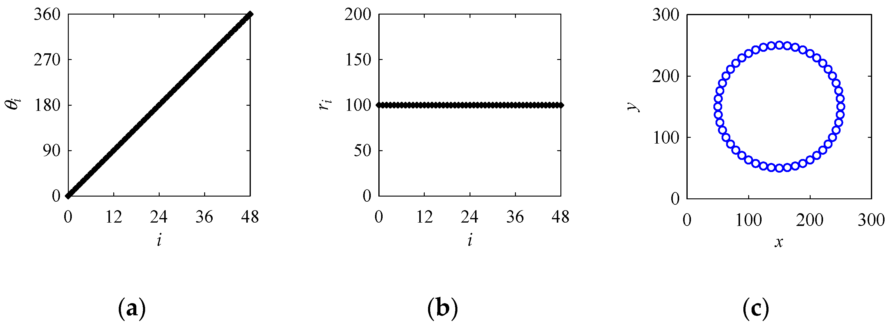
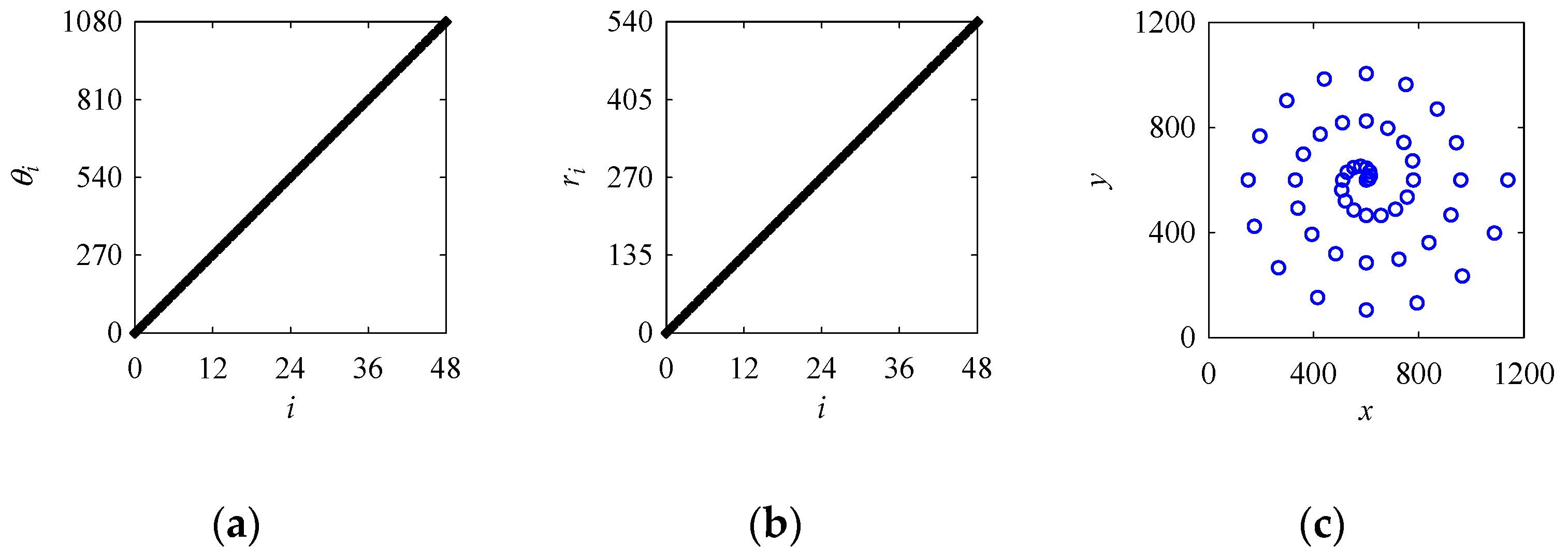
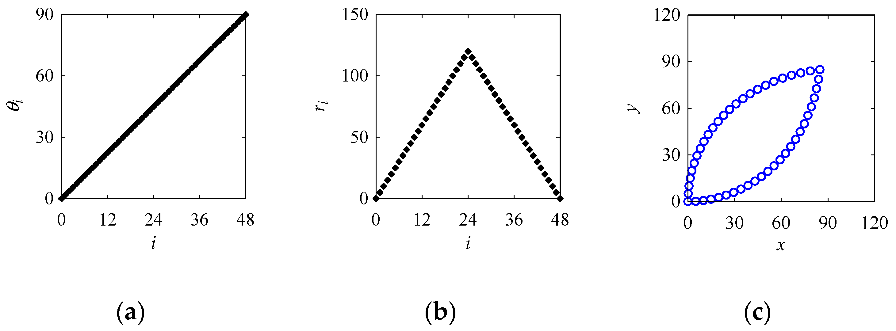
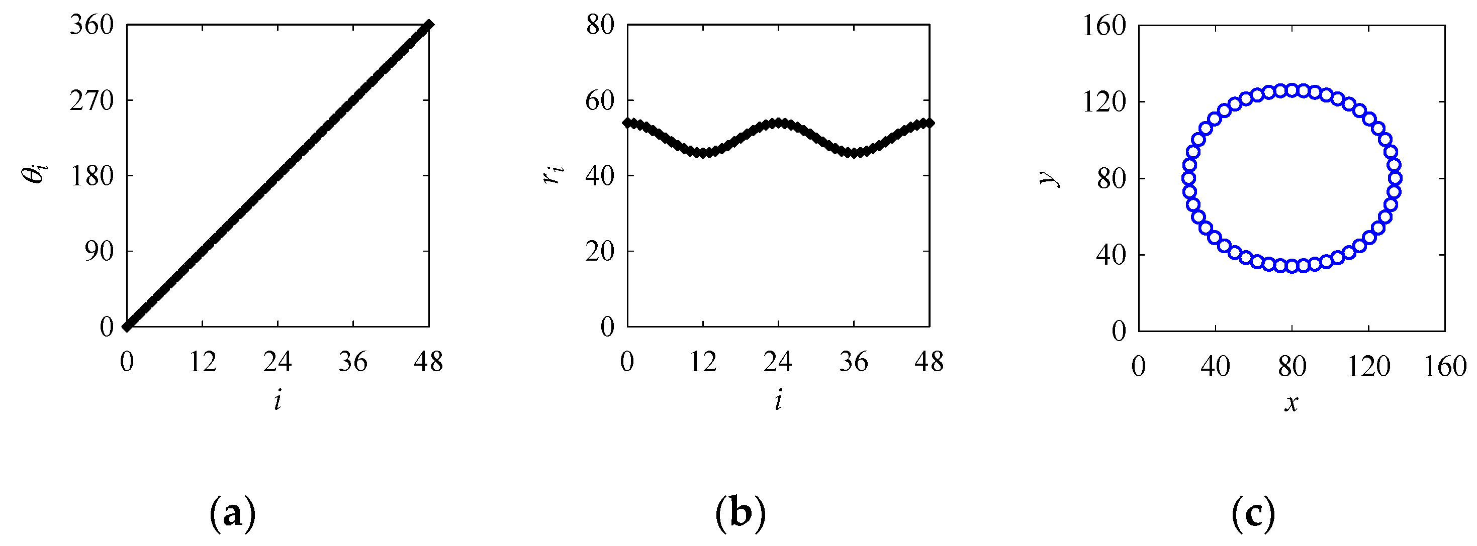
2. Characteristics of the Point-Cloud-Creating Algorithm

Recall the following question. What are the characteristics and roles of the variables and constants used in the recursive process that deterministically creates a point cloud? The recursive process, called the point cloud creation algorithm (PCA), that creates a point cloud on a plane is shown in Appendix A. As shown in Appendix A, PCA needs three constants as inputs—namely, the center point, Pc; initial distance, d; and initial angle, φ—that remain the same for all iterations. In addition, PCA needs two variables as inputs—namely, instantaneous rotational angle, θi and instantaneous distance, ri, i = 0, 1, ..., n—that may change in every iteration. The PCA creates the output, denoted as PC = {Pei | i = 0, 1, ..., n}, which is a small-size point cloud. As such, the output of PCA, PC depends on d, φ, θi, and ri. This input–output relationship is characterized by using some well-known shapes, namely, straight-line, circle, ellipse, spiral, astroid, S-shape, and leaf-shape. The description is as follows.
First, consider the point clouds that evolve due to the linear settings of the instantaneous rotational angle and distance. These settings create some point clouds presenting straight lines, circles, and spirals, as shown in Figure 2, Figure 3, Figure 4 and Figure 5. For example, consider a point cloud that models a straight line. In this case, θi must be kept constant and ri must linearly increase or decrease. When θi = 0° and ri linearly increases for all iterations, the PCA creates a point cloud, PC, presenting a horizontal line, as shown in Figure 2. When θi = 90° and ri linearly increases for all iterations, the PCA creates, PC, presenting a vertical line, as shown in Figure 3. The slope of the straight line can be modeled using θi. When an opposite strategy is adopted, that is, θi is increased or decreased linearly and ri is kept constant, the point cloud, PC, presents a shape called a circle, as shown in Figure 4. In this case, the radius of the circle can be modeled using ri. On the other hand, when both θi and ri are increased or decreased simultaneously, then the point cloud, PC, presents a shape called a spiral, as shown in Figure 5.
In the next step, consider the relatively complex settings of the instantaneous distance while keeping the instantaneous rational angle increase linear. For example, when θi is increased linearly and ri follows a tent function, then the point cloud, PC, presents a shape called leaf-shape, as shown in Figure 6. When θi increases linearly and ri follows a sine or cosine function with two cycles, then the point cloud, PC, presents a shape called ellipse, as shown in Figure 7. Similarly, when θi increases linearly and ri follows a u-shape function with four cycles, then the point cloud, PC, presents a shape called astroid, as shown in Figure 8. When θi increases linearly and ri follows a bathtub function with two cycles, then the point cloud, PC, presents a shape called S-shape, as shown in Figure 9. As shown in Figure 2, Figure 3, Figure 4, Figure 5, Figure 6, Figure 7, Figure 8 and Figure 9, keeping θi very simple (constant or straight-line) and varying ri using some simple functions (straight-line, tent function, sine/cosine, u-shape function, and bathtub functions) can model a variety of shapes. The findings are summarized in Table 1. These characteristics of the algorithm can be used while modeling an arbitrary planner shape or a segment of it.
As shown in Table 1, besides the instantaneous rotational angle and distance described above, the other input parameters of the PCA, the center point, Pc and the initial angle, φ also play an important role. For instance, the leaf-shape shown in Figure 9 can be rotated by resetting the values of φ. For example, when the initial angle is set in the following manner φ = 0°, 45°, and 90°, the leaf-shape shown in Figure 6 rotates by 0°, 45°, and 90°, respectively, as shown in Figure 10. Similarly, Pc can perform the function of translation in both x-axis and y-axis directions. The initial distance, d, on the other hand, does not play many roles, i.e., it does not affect the shape to be modeled; it is only necessary for placing the starting point.

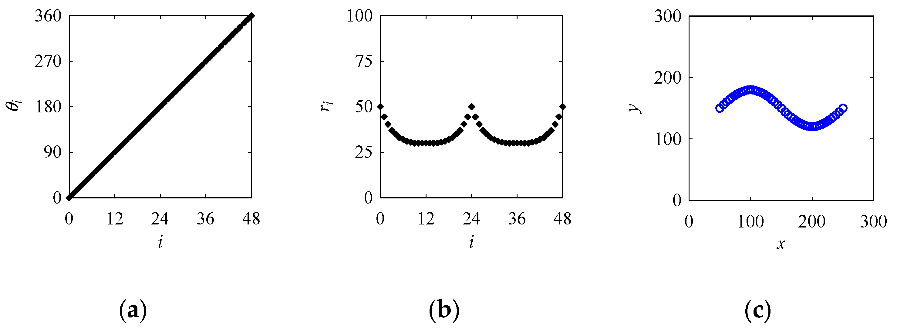
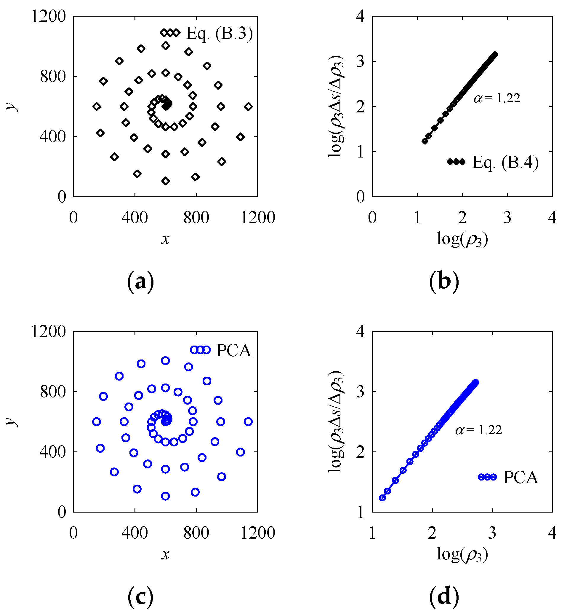
3. Quantification of Point Clouds

Recall the following questions. How do we quantify the shape information modeled by a set of a point cloud? Does the recursive process that deterministically creates a point cloud correctly model a given shape?
In order to answer the abovementioned questions, two well-known parameters called a radius of curvature and aesthetic value, defined in Appendix B, are considered.
Let A be a planner shape. Let U be a method that creates a point cloud V = {Vi | i = 0, 1, …} to model A. In addition, PC = {Pei | i = 0, 1, ...} is created by PCA to model A. As such, both point clouds, V = {Vi | i = 0, 1, …} and PC = {Pei | i = 0, 1, ...} must look alike. At the same time, their quantitative characteristics must be the same. Based on this consideration, this section quantifies two point clouds of the same shape using the radius of curvature and aesthetic value, respectively.

3.1. Quantification Based on Radius of Curvature

Consider the parameter called a radius of curvature [73], as defined in Appendix B. A point in a point cloud has a radius of curvature, ρi, i = 0, 1, …. To calculate ρi, the point itself and two more preceding consecutive points are needed. The variability in ρi is calculated for circle, ellipse, and spiral, as shown in Figure 11, Figure 12 and Figure 13.
Figure 11 shows two point clouds of the same shape, circle. Figure 11a shows the point cloud of the circle modeled by Equation (A1), where the radius, a = 100 and center, Pc = (150,150). In this case, 49 points are created to model the circle. Figure 11b shows the values of ρi, which is equal to 100.21. Theoretically, ρi must be equal to a = 100. This small error (100.21 – 100 = 0.21) is due to calculation precision error. On the other hand, Figure 11c shows the point cloud of the same circle modeled by a PCA-generated point cloud. For this point cloud, ri = 100 (= d); φ = 0; θi = 2πi/n; n = 48; i = 0, 1, …, 48; and Pc = (150, 150). In this case as well, 49 points are created to model the circle. Figure 11d shows the values of ρi, which is equal to 100.21. This means that for a circle, ri plays the role of the radius of curvature of a circle.
Figure 12 shows two point clouds of the same shape, ellipse. Figure 12a shows the point cloud of the ellipse modeled by Equation (A2), where the major radius, a = 54; minor radius, b = 46; and center, Pc = (80, 80). In this case, 49 points are created to model the ellipse. Figure 12b shows the variation of ρi. On the other hand, Figure 12c shows the point cloud of the same ellipse modeled by a PCA-generated point cloud. For this point cloud, d = 15; φ = 0; ri is decreased linearly from 54 to 46 and increased linearly from 46 to 56 for two cycles; θi = 2πi/n; n = 48; i = 0, 1, …, 48; and Pc = (80, 80). In this case as well, 49 points are created to model the ellipse. Figure 12d shows the variation of ρi. As seen in Figure 12a,c, it is clear that both point clouds are identical and their radius of curvature (Figure 12b,d) also varies in the same trend. This means that for an ellipse, ri plays the role of the radius of curvature of an ellipse.
Figure 13 shows two point clouds of the same shape, spiral. Figure 13a shows the point cloud of the spiral modeled by Equation (A3), where an arbitrary, positive, real constant, a = 28.647 that controls the distance between the successive turnings of the spiral. In this case, 49 points are created to model the spiral. Figure 13b shows the variation of ρi. On the other hand, Figure 13c shows the point cloud of the same spiral modeled by a PCA-generated point cloud. For this point cloud, d = 15; φ = 0; ri = 0, 11.25, …, 540; θi = 2πi/n; n = 48; i = 0,1, …, 48; and Pc = (600, 600). In this case as well, 49 points are created to model the spiral. Figure 13d shows the variation of ρi. As seen in Figure 13a,c, it is clear that both point clouds are identical and their radius of curvature (Figure 13b,d) also varies in the same trend. This means that for spiral, ri plays the role of a radius of curvature of a spiral.
It is clear from Figure 11, Figure 12 and Figure 13, the shape modeled by the parametric equation based and the PCA are visually identical. This means that the instantaneous distance plays the role of the radius of curvature when the shape is modeled by the PCA. The variation of the instantaneous distance is comparatively lower than the radius of curvature, which shows that the geometry of the shape can be easily controlled using the instantaneous distance compared to the radius of curvature. It is worth mentioning that there are several key elements for shape designing, and mathematical formulation of the radius of curvature or instantaneous distance can be one effective approach [74].

3.2. Quantification Based on Aesthetic Value

This subsection describes the quantification of shapes based on a parameter called aesthetic value, denoted as α [75,76,77]. This parameter is defined in Appendix B. In order to know the aesthetic value, a plot called a logarithm curvature histogram (LCH) is used. The procedure to construct LCH for a given curve (in this case from a given point cloud) is also shown in Appendix B. For quantification of the aesthetic value, the ellipse and spiral shape are considered.
Figure 14a shows the point cloud of the ellipse modeled by Equation (A2), which is repeated from the previous section (Figure 12a). The corresponding LCH of the ellipse is shown in Figure 14b. Figure 14c shows the point cloud of the ellipse modeled by the PCA (repeated from Figure 12c). The corresponding LCH of the ellipse is shown in Figure 14d. Both point clouds have the same aesthetic value, α = 1.25. On the other hand, Figure 15a shows the point cloud of a spiral modeled by Equation (A3) (repeated from Figure 13a). The corresponding LCH of the spiral is shown in Figure 15b. Figure 15c shows the point cloud of the spiral modeled by the PCA (repeated from Figure 13c). The corresponding LCH of the spiral is shown in Figure 14d. Both point clouds of the spiral shape have the same aesthetic value, α = 1.22. As seen in Figure 14 and Figure 15, even though the shapes are created using the PCA instead of the respective parametric equations, their aesthetic natures remain unaffected. It is also observed that the length of the line segment in the LCH depends on the variation range (minimum value to maximum value) of the radius of curvature. If the variation in the radius of curvature is high, the length of LCH becomes larger and vice versa.

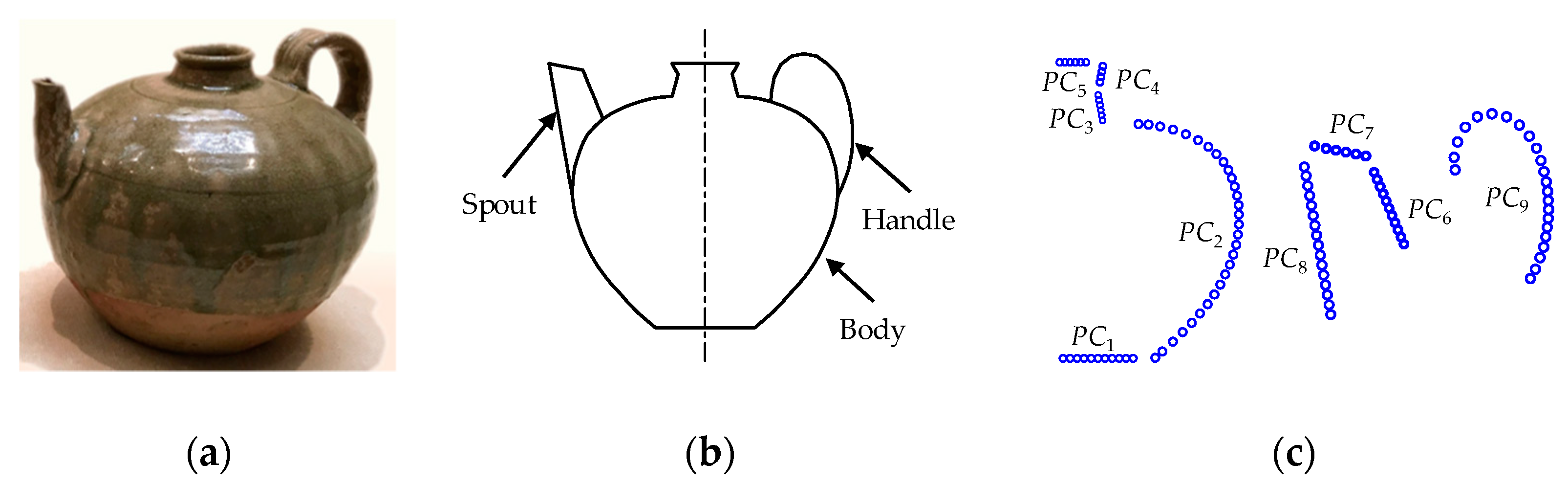
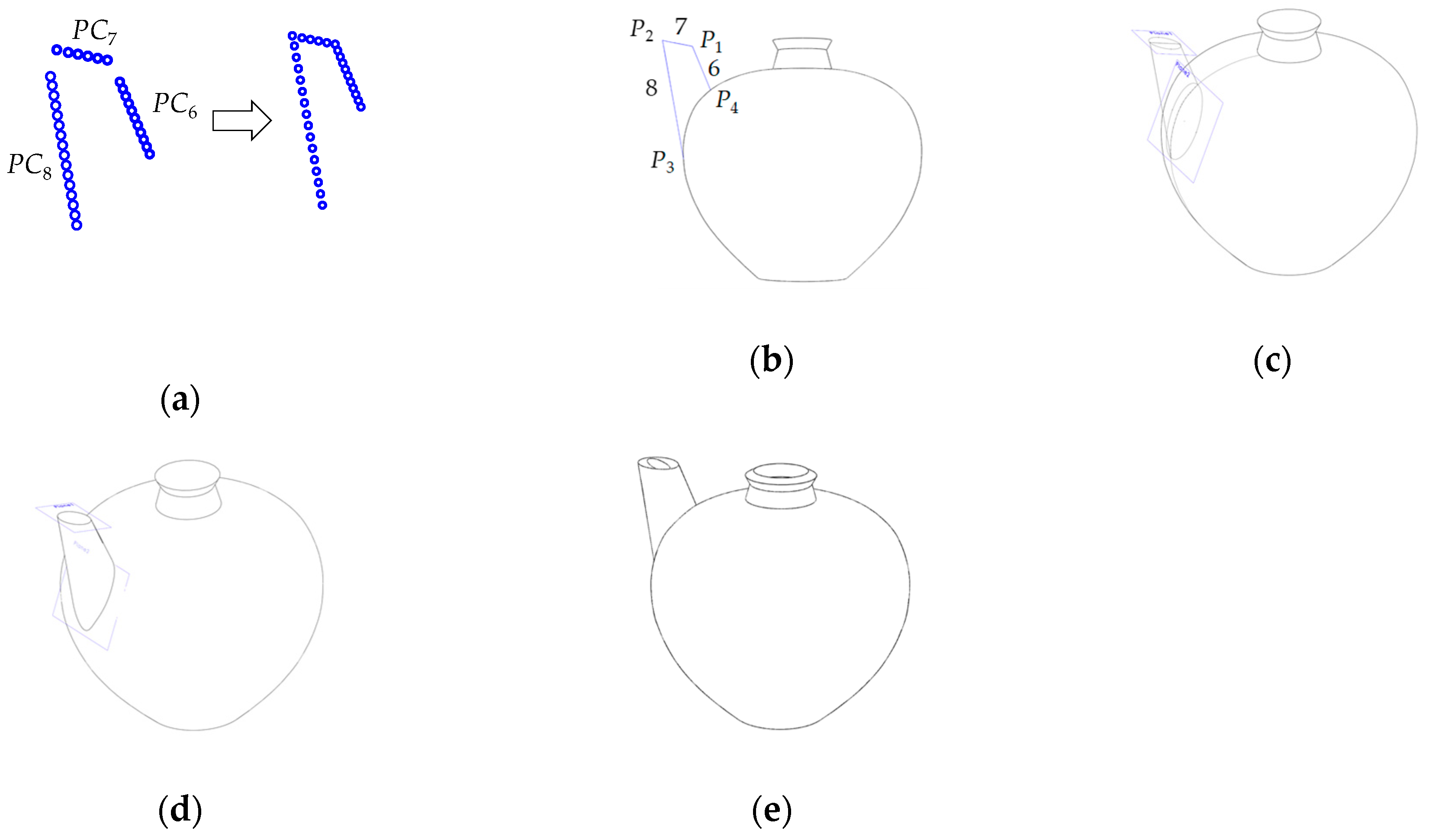
4. 3D Solid Modeling and Physical Prototyping

Recall the last question, as follows. Does the deterministically created point cloud help create 3D solid models of some given objects?
In order to answer this question, this section presents an illustrative example where a relatively complex object is first modeled by some point clouds. The point clouds are generated by the PCA. The point clouds are used in a sequential order to produce a solid model of the object within a CAD package. Finally, a physical prototype is built from digital data of the solid model.
Figure 16a shows an ewer from Seto ware (Seto is a city located in Aichi Prefecture, Japan) produced during the Nanboku-chō period in the 13th century [78]. The ewer consists of three parts—the body, spout, and handle—as shown in Figure 16b. Few line segments and a concave can represent the body, line segments can represent the spout, and an elliptical shape can represent the handle. Hence, the ewer can be constructed using line segments, a concave curve, and an ellipse. Figure 16c shows the individual point clouds modeled by the PCA. Consider the individual point clouds, PC1, PC3, PC4, PC5, PC6, PC7, and PC8, presenting the line segments that can be modeled by customizing the inputs, θi and ri, as described in Section 2 (Figure 2 and Figure 3). Similarly, consider the point cloud PC9, presenting an elliptical shape that can be modeled by customizing the inputs, θi and ri, as described in Section 2 (Figure 7). Regarding the point cloud PC2, presenting the concave curve that can be modeled by setting the input parameters of the PCA as follows: PC = (90,90); d = 15; φ = 0; θi = πi/2n, n = 30; i = 0,1, …, 30; and ri is linearly decreased from 73.55 to 0.
The steps for solid CAD modeling are described as follows. In the first step, the individual point clouds PC1, PC2, PC3, PC4, and PC5 are sequentially synthesized by a C0 continuity approach which represents the basic point cloud of the ewer body. The resulting point cloud is shown in Figure 17a. These point clouds are then transferred to a commercially available 3D CAD package for solid modeling. By revolving the point cloud 360°, a solid CAD model of the ewer body is constructed. The result is shown in Figure 17b.
In the second step, the point clouds PC6, PC7, and PC8 are sequentially synthesized by a C0 continuity approach which represents the basic point cloud of the spout. The resulting point cloud is shown in Figure 18a. The point clouds are then injected into the solid CAD model of the body as shown in Figure 18b. Here, P1 and P2 represent the start point and endpoint of PC7 and are connected to the endpoint of PC6 and start point of PC8, respectively. For the other points, P3 denotes the endpoint of PC8 and P4 denotes the starting point of PC6. The point clouds must be iterated so that P3 and P4 must lie on a tangent to the surface of the body. Taking P1 and P2 as reference points, plane 1 is created and then an ellipse is constructed on plane 1, as shown in Figure 18c. Similarly, taking P3 and P4 as reference points, plane 2 is created and then another ellipse is constructed on plane 2, as shown in Figure 18c. Now, these two ellipses are joined by applying the lofted function to form the spout, as shown in Figure 18d. Afterward, a hollow is created inside the solid CAD model by offsetting surface and hiding the solid body and applying the thicken function on the offset surface. The resulting solid CAD model is shown in Figure 18e.
In the third step, the point cloud PC9, shown in Figure 19a, is injected on the solid CAD model, as shown in Figure 19b. In this case, PC9 must iterate so the start point P5, and endpoint P6, must lie on the mid-section of the outer and inner surface of the body, shown in Figure 19b. Taking P5 and PC9 as a reference, plane 3 is created and then the ellipse is constructed on plane 3, as shown in Figure 19c. Then, applying the sweep function on the ellipse and taking PC9 as a sweep path, a handle is created. The resulting solid CAD model is shown in Figure 19d.
Finally, the rendered solid CAD model of the ewer is shown in Figure 20a. Once the solid CAD modeling is done, triangulation modeling is performed simply by saving the solid CAD model into an STL data file using a CAD package. Figure 20b shows the triangulation model of the ewer. The STL data generated from the triangulation modeling can be used to build a physical model using commercially available 3D printing devices (e.g., 3D printer). Figure 20b shows one of the ewer physical models built by a 3D printer available at the Kitami Institute of Technology.

5. Discussions

The above three sections answer the questions coined in the introduction. Apart from this, the presented methodology can be used in many different ways. One of the ways is surface texturing. This section provides some insights into this type of surface texturing.
The PCA-based point cloud can be used for surface texturing. For example, consider the solid model of the ewer shown in Figure 20. A texture can be added to it. In this case, the PCA-based point cloud can be used. For example, consider the point clouds that represent a pattern taken from Ainu cultural heritage. The settings for creating the point clouds are available in [69].
Figure 21a shows the point cloud of the texture. This point cloud is injected into the solid CAD model of the ewer, as shown in Figure 21b. Then, the texture on the front side is constructed by extruding the point cloud from the surface of the ewer. The texture on the backside is constructed by mirroring the front side texture. The result is shown in Figure 21c. Finally, the physical model is realized using a 3D printer, as shown in Figure 21d.
In addition to texturing, the 3D printed physical model of ewer shown in Figure 21 is scanned using a 3D scanner available at the Kitami Institute of Technology. Three different orientations are implemented to scan the ewer, as shown in Figure 22. Point clouds are then preprocessed (removing noise points, removing redundant points, and combining all point clouds into a single coordinate) and a triangulation model is created directly from the point cloud. The triangulation model is shown in Figure 22. Afterwards, a solid CAD model is constructed from the triangulation model. As seen in Figure 23a, the texture is a blur and there is also surface distortion near the handle. To make the texture sharp, clear, and have a smooth surface, it requires the user efforts while performing solid CAD modeling. It is worth mentioning that the triangulation model from the 3D scanned point cloud (Figure 23) consists of 271,803 facets and 815,409 vertices, whereas the triangulation model from the PCA-based point cloud has 25,336 facets and 76,008 vertices for the model without texture (Figure 20b); and 51,244 facets and 153,732 vertices for the model with texture (Figure 21d). It is clear that the 3D scanned point cloud has 10 times higher facets than the PCA-based point cloud. As a result, the 3D scan-based approach becomes user-dependent and requires heavy computation. Table 2 shows a summary of the number of points, facets, vertices, and printing time required to manufacture the physical model of the given ewer.
The article has demonstrated geometric modeling of a given shape which is completely controlled by a few analytically generated points and free from computational complexity. This way, the user has the freedom to design any given shape without being dependent on the data acquisition system. Moreover, the point clouds are used in a sequential order to produce the solid CAD model of the given object.

6. Concluding Remarks

In this article, the characteristics and roles of the two variables (instantaneous distance and instantaneous rotational angle) and three constants (center point, initial angle, and initial distance) used in the recursive process that deterministically creates a point cloud are studied. It is found that varying the pair of the instantaneous distance and instantaneous rotational angle in different combinations can create many different shapes. For examples, in this study, a straight-line, circle, ellipses, spiral, astroid, S-shape, and leaf-shape are created using five different combinations of instantaneous distance and instantaneous rotational angle. The first constant (center point) can perform the function of translation in both x- and y-axis directions. The second constant (initial angle) can perform the function of rotation of shape around the center point. However, the third constant does not affect the shape to be modeled; it is only necessary for placing the starting point.
A planner shape can be modeled by a recursive-process-created point cloud and by a parametric-equation-created point cloud. If both point clouds are the same in terms of some quantitative measures, then it can be said that the recursive-process-based shape modeling approach is as good as the parametric-equation-based shape modeling approach. This is verified using three well-known shapes, namely, circle, ellipse, and spiral. In the verification process, the parameters called the radius of curvature and aesthetic value are used. It is observed that both point clouds of a given shape (one generated by the recursive process and the other generated by the parametric equation) have the same radius of curvature and aesthetic value. It is also found that the instantaneous distance plays the role of a radius of curvature. This means that it is not difficult to predict the values of the instantaneous distance compared to those of the radius of curvature while modeling an arbitrary shape.
In addition, an illustrative example that shows the efficacy of the recursive process in virtual and physical prototyping of a relatively complex 3D object is presented. The results show that, compared to a 3D-scanner-created point cloud, the recursive-process-created point cloud helps avoid computational complexity in reverse engineering. It also makes reverse engineering more systematic of complex shape. Moreover, the recursive-process-created point cloud can be used to perform surface texturing.
In the future, this study can be extended to develop a system that automatically generates a shape based on the user-defined inputs (instantaneous distance and rotational angle, and alike). This way, human cognition-based reverse engineering can be achieved—which is one of the frontiers of digital manufacturing.

Author Contributions

Tashi, A.M.M.S.U., and A.K. conceived the idea. Tashi and A.M.M.S.U. worked on the methodology and manuscript preparation. Tashi and A.K. conducted the scanning experiment in Section 5. Tashi and AM.M.S.U. produced the point cloud and solid CAD models. A.M.M.S.U. administered the work.

Acknowledgments

The authors acknowledge Kitami Institute of Technology for providing materials and financial support during the course of this study.

Conflicts of Interest

The authors declare no conflicts of interest.

Appendix A. Point Cloud Creation Algorithm

The PCA needs three constants, namely, the center point (Pc), initial distance (d), and the initial angle (φ), that remain the same during the iterations. In addition, the PCA needs two variables—namely, the instantaneous rotational angle (θi) and instantaneous distance (ri), i = 0, 1, ..., n—that change in every iteration. The PCA consists of four steps. The first is input, the second is calculation, the third is iteration, and the last is output. In the input step, Pc = (Pcx, Pcy) ∈ 2; d > 0; φ; ri | i = 0, 1, ..., n); and θi | i = 0, 1, ..., n are defined. In the calculation step, an initial point P0 = (P0x, P0y) is calculated first at distance d from Pc on line PcP0, making angle φ in the counterclockwise direction with the x-axis. In the iteration step, P0 is rotated counterclockwise from the x-axis using θi to create points Pi = (Pix, Piy), i = 0, 1, …, n. Afterward, points Pi = (Pix, Piy) are placed at a distance ri from Pc resulting in points Pei = (Pix, Piy), i = 0, 1, ..., n. In the output step, the points Pei = (Pix, Piy), i = 0, 1, ..., n, are collected for creating the desired point cloud denoted as PC = {Pei | i = 0, 1, ..., n}.
Point Cloud Creation Algorithm (PCA):
1Define:Center Point Pc = (Pcx, Pcy) ∈ 2, Initial Length d > 0, Initial Angle φ
Instantaneous Distance (ri | i = 0, 1, ..., n)
Instantaneous Rotational Angle (θi | i = 0, 1, ..., n)
2Calculate:P0 = (P0x, P0y) so that P 0 x = P c x + d cos ϕ and P 0 y = P c y + d sin ϕ
3Iterate:For i = 0, 1, ..., n
  • Rotate P0 by an angle θi around Pc in the counterclockwise direction to create Pi = (Pix, Piy) so that
    P i x = P c x + ( P 0 x P c x ) cos θ i ( P 0 y P c y ) sin θ i ,
    P i y = P c y + ( P 0 x P c x ) sin θ i + ( P 0 y P c y ) cos θ i .
  • Extend Pi to Pei (a point on the line PcPi at a distance ri from Pc)
    P e i x = P c x + ( P i x P c x ) ( r i / d ) ,
    P e i y = P c y + ( P i y P c y ) ( r i / d ) .
End For
4Output:PC = (Pei | i = 0, 1, ..., n)

Appendix B. Definition of Relevant Shapes and Parameters

B.1. Relevant Shapes

Let the point clouds of a circle, ellipse, and spiral be modeled by three parametric equations. Each shape is given by a point cloud consisting of the points Pi = {(Pxi, Pyi) | i = 0, 1, …, n. The mathematical formulations of the shapes are as follows.
Consider a circle with radius a, where a > 0. Let Pc = (Pcx, Pcy) be the center of the circle on the xy plane. An arbitrary point on the circumference of the circle is denoted as Pi = {(Pxi, Pyi) | i = 0, 1, …, n} and is given by
P x i = P c x + a cos θ i ,     P y i = P c y + a sin θ i .
In Equation (A1), θi = 2πi/n. While creating a point cloud for a circle using Equation (A1), the parameters are set as follows: a = 100; n = 48; and i = 0, 1, ..., 48. The point cloud shown in Figure 11a presenting the circle is created using the abovementioned formulation.
Consider an ellipse with major radius a and minor radius b, where a, b > 0 and a > b. Let Pc = (Pcx, Pcy) be the center of the ellipse in the xy plane. An arbitrary point on the circumference of the ellipse is denoted as Pi = {(Pxi, Pyi) | i = 0, 1, …, n} and is given by
P x i = P c x + a cos θ i ,     P y i = P c y + b sin θ i .
In Equation (A2), θi = 2πi/n. While creating a point cloud for an ellipse using Equation (A2), the parameters are set as follows: a = 54; b = 46; n = 48; and i = 0, 1, ..., 48. The point cloud shown in Figure 12a presenting the ellipse is created using the abovementioned formulation.
Consider a spiral. Let it be an Archimedean spiral. Let PC = (Pcx, Pcy) be the center of the spiral in the xy plane. Consider a to be the arbitrary positive real constant that controls the distance between the successive turnings of the spiral. An arbitrary point on the circumference of the spiral is denoted as Pi = {(Pxi, Pyi) | i = 0, 1, …, n} and is given by
P x i = P c x + a θ i cos θ i ,     P y i = P c y + a θ i sin θ i .
In Equation (A3), θi = 6πi/n. While creating a point cloud for a spiral using Equation (A3), the parameters are set as follows: a = 28.647; n = 48; and i = 0, 1, ..., 48. The point cloud shown in Figure 13a presenting the spiral is created using the abovementioned formulation.

B.2. Radius of Curvature

Let ρi be the instantaneous radius of curvature for point Pi = {(Pxi, Pyi) | i = 0, 1, …, n}. Thus, the following relationship holds [73]:
ρ i = ( ( x ˙ i ) 2 + ( y ˙ i ) 2 ) 3 / 2 | ( ( x ˙ i ) ( y ¨ i ) ( y ˙ i ) ( x ¨ i ) ) | .
In Equation (A4), i = Pxi+1Pxi; i = Pyi+1Pxy; i = i+1i; and ÿi = i+1i. The radii of curvature for the shapes described above are computed using Equation (A4).

B.3. Aesthetic Value

A parameter called aesthetic value, denoted as α, quantifies the aesthetic nature of a curve [75,76,77], which is driven from the radius of curvature (Equation (A4)) and the arc length of a given curve, as shown in Figure A1. As seen in Figure A1a, ρ, Δs, and Δρ are the radius of curvature, arc length, and change in the radius of curvature, respectively. The logarithmic plot of Δs/(Δρ/ρ) versus ρ, which is called Logarithmic Curvature Histogram (LCH), becomes a straight line, and its slope is used to calculate the value of α, as seen in Figure A1b. Therefore, the following relationship holds [76]:
log ( Δ s Δ ρ / ρ ) = α log ( ρ ) + c .
In Equation (A5), c is a constant. By knowing the value of α, the degree of aesthetics of a given curve (shape) can be quantified.
Figure A1. Determining aesthetic value. (a) Parameters for determining the aesthetic value; (b) calculating aesthetic value using LCH.
Mca 24 00083 g0a1

References

  1. Thompson, M.K.; Moroni, G.; Vaneker, T.; Fadel, G.; Campbell, R.I.; Gibson, I.; Bernard, A.; Schulz, J.; Graf, P.; Ahuja, B.; et al. Design for Additive Manufacturing: Trends, opportunities, considerations, and constraints. CIRP Ann. 2016, 65, 737–760. [Google Scholar] [CrossRef]
  2. Gibson, I.; Rosen, D.; Stucker, B. Additive Manufacturing Technologies: 3D Printing, Rapid Prototyping, and Direct Digital Manufacturing, 2nd ed.; Springer-Verlag: New York, NY, USA, 2015. [Google Scholar]
  3. Gao, W.; Zhang, Y.; Ramanujan, D.; Ramani, K.; Chen, Y.; Williams, C.B.; Wang, C.C.L.; Shin, Y.C.; Zhang, S.; Zavattieri, P.D. The status, challenges, and future of additive manufacturing in engineering. Comput. Aided Des. 2015, 69, 65–89. [Google Scholar] [CrossRef]
  4. Tofail, S.A.M.; Koumoulos, E.P.; Bandyopadhyay, A.; Bose, S.; O’Donoghue, L.; Charitidis, C. Additive manufacturing: scientific and technological challenges, market uptake and opportunities. Mater. Today 2018, 21, 22–37. [Google Scholar] [CrossRef]
  5. Nooran, R. 3D Printing: Technology, Applications, and Selection, 1st ed.; CRC Press: Boca Raton, FL, USA, 2018. [Google Scholar]
  6. Camille, B. What are you printing? Ambivalent emancipation by 3D printing. Rapid Prototyp. J. 2015, 21, 572–581. [Google Scholar]
  7. Bourell, D.L.; Rosen, D.W.; Leu, M.C. The Roadmap for Additive Manufacturing and Its Impact. 3D Print. Addit. Manuf. 2014, 1, 6–9. [Google Scholar] [CrossRef]
  8. Hirz, M.; Rossbacher, P.; Gulanová, J. Future trends in CAD—From the perspective of automotive industry. Comput. Aided Des. Appl. 2017, 14, 734–741. [Google Scholar] [CrossRef]
  9. Yap, Y.L.; Tan, Y.S.E.; Tan, H.K.J.; Peh, Z.K.; Low, X.Y.; Yeong, W.Y.; Tan, C.S.H.; Laude, A. 3D printed bio-models for medical applications. Rapid Prototyp. J. 2017, 23, 227–235. [Google Scholar] [CrossRef]
  10. Hieu, L.C.; Zlatov, N.; Vander Sloten, J.; Bohez, E.; Khanh, L.; Binh, P.H.; Oris, P.; Toshev, Y. Medical rapid prototyping applications and methods. Assembly Autom. 2005, 25, 284–292. [Google Scholar] [CrossRef]
  11. Sun, W.; Starly, B.; Nam, J.; Darling, A. Bio-CAD modeling and its applications in computer-aided tissue engineering. Comput. Aided Des. 2005, 37, 1097–1114. [Google Scholar] [CrossRef]
  12. Mannoor, M.S.; Jiang, Z.; James, T.; Kong, Y.L.; Malatesta, K.A.; Soboyejo, W.O.; Verma, N.; Gracias, D.H.; McAlpine, M.C. 3D Printed Bionic Ears. Nano Lett. 2013, 13, 2634–2639. [Google Scholar] [CrossRef] [Green Version]
  13. Steffan, D.; Dominic, E. A CAD and AM process for maxillofacial prostheses bar-clip retention. Rapid Prototyp. J. 2016, 22, 170–177. [Google Scholar]
  14. Luximon, Y.; Ball, R.M.; Chow, E.H.C. A design and evaluation tool using 3D head templates. Comput. Aided Des. Appl. 2016, 13, 153–161. [Google Scholar] [CrossRef]
  15. Jung, W.; Park, S.; Shin, H. Combining volumetric dental CT and optical scan data for teeth modeling. Comput. Aided Des. 2015, 67, 24–37. [Google Scholar] [CrossRef]
  16. Urbanic, R.J. From thought to thing: using the fused deposition modeling and 3D printing processes for undergraduate design projects. Comput. Aided Des. Appl. 2016, 13, 768–785. [Google Scholar] [CrossRef]
  17. Galina, L.; Na, X. Academic library innovation through 3D printing services. Libr. Manag. 2017, 38, 208–218. [Google Scholar] [Green Version]
  18. Heather, M.M.L. Makers in the library: case studies of 3D printers and maker spaces in library settings. Libr. Hi Tech 2014, 32, 583–593. [Google Scholar]
  19. Wannarumon, S.; Bohez, E.L.J. A New Aesthetic Evolutionary Approach for Jewelry Design. Comput. Aided Des. Appl. 2006, 3, 385–394. [Google Scholar] [CrossRef]
  20. 3D Printed Clothing. Available online: https://3dprint.com/tag/3d-printed-clothing/ (accessed on 13 September 2019).
  21. The Future of Running is Here. Available online: https://www.newbalance.com/article?id=4041 (accessed on 13 September 2019).
  22. 3D Printed Fashion: 10 Amazing 3D Printed Dresses. Available online: https://i.materialise.com/blog/3d-printed-fashion-dresses/ (accessed on 13 September 2019).
  23. Nike. Nike Debuts First-ever Football Cleat Built Using 3D Printing Technology. Available online: https://news.nike.com/news/nike-debuts-first-ever-football-cleat-built-using-3d-printing-technology (accessed on 13 September 2019).
  24. Sun, J.; Zhou, W.; Yan, L.; Huang, D.; Lin, L.Y. Extrusion-based food printing for digitalized food design and nutrition control. J. Food Eng. 2018, 220, 1–11. [Google Scholar] [CrossRef]
  25. Lin, C. 3D Food Printing: A Taste of the Future. J. Food Sci. Educ. 2015, 14, 86–87. [Google Scholar] [CrossRef] [Green Version]
  26. Ferreira, I.A.; Alves, J.L. Low-cost 3D food printing. Ciência Tecnologia dos Materiais 2017, 29, e265–e269. [Google Scholar] [CrossRef]
  27. Jiang, H.; Zheng, L.; Zou, Y.; Tong, Z.; Han, S.; Wang, S. 3D food printing: Main components selection by considering rheological properties. Crit. Rev. Food Sci. Nutr. 2019, 59, 2335–2347. [Google Scholar] [CrossRef] [PubMed]
  28. Lupton, D.; Turner, B. Food of the Future? Consumer Responses to the Idea of 3D-Printed Meat and Insect-Based Foods. Food Foodways 2018, 26, 269–289. [Google Scholar] [CrossRef]
  29. Sakin, M.; Kiroglu, Y.C. 3D Printing of Buildings: Construction of the Sustainable Houses of the Future by BIM. Energy Procedia 2017, 134, 702–711. [Google Scholar] [CrossRef]
  30. Hager, I.; Golonka, A.; Putanowicz, R. 3D Printing of Buildings and Building Components as the Future of Sustainable Construction? Procedia Eng. 2016, 151, 292–299. [Google Scholar] [CrossRef] [Green Version]
  31. Lim, S.; Buswell, R.A.; Le, T.T.; Austin, S.A.; Gibb, A.G.F.; Thorpe, T. Developments in construction-scale additive manufacturing processes. Autom. Constr. 2012, 21, 262–268. [Google Scholar] [CrossRef] [Green Version]
  32. Tay, Y.W.D.; Panda, B.; Paul, S.C.; Noor Mohamed, N.A.; Tan, M.J.; Leong, K.F. 3D printing trends in building and construction industry: A review. Virtual Phys. Prototyp. 2017, 12, 261–276. [Google Scholar] [CrossRef]
  33. Scopigno, R.; Cignoni, P.; Pietroni, N.; Callieri, M.; Dellepiane, M. Digital Fabrication Techniques for Cultural Heritage: A Survey. Comput. Graph. Forum 2017, 36, 6–21. [Google Scholar] [CrossRef]
  34. Sharif Ullah, A.M.M.; Sato, Y.; Kubo, A.; Tamaki, J.i. Design for Manufacturing of IFS Fractals from the Perspective of Barnsley’s Fern-leaf. Comput. Aided Des. Appl. 2015, 12, 241–255. [Google Scholar] [CrossRef]
  35. Várady, T.; Martin, R.R.; Cox, J. Reverse engineering of geometric models—An introduction. Comput. Aided Des. 1997, 29, 255–268. [Google Scholar] [CrossRef]
  36. James, D.W.; Belblidia, F.; Eckermann, J.E.; Sienz, J. An innovative photogrammetry color segmentation based technique as an alternative approach to 3D scanning for reverse engineering design. Comput. Aided Des. Appl. 2017, 14, 1–16. [Google Scholar] [CrossRef]
  37. Paulic, M.; Irgolic, T.; Balic, J.; Cus, F.; Cupar, A.; Brajlih, T.; Drstvensek, I. Reverse Engineering of Parts with Optical Scanning and Additive Manufacturing. Procedia Eng. 2014, 69, 795–803. [Google Scholar] [CrossRef] [Green Version]
  38. Ullah, A.M.M.; Watanabe, M.; Kubo, A. Analytical Point-Cloud Based Geometric Modeling for Additive Manufacturing and Its Application to Cultural Heritage Preservation. Appl. Sci. 2018, 8, 656. [Google Scholar] [Green Version]
  39. Furferi, R.; Governi, L.; Volpe, Y.; Puggelli, L.; Vanni, N.; Carfagni, M. From 2D to 2.5D i.e. from painting to tactile model. Graph. Models 2014, 76, 706–723. [Google Scholar] [CrossRef]
  40. Rojas-Sola, J.I.; Galán-Moral, B.; De la Morena-De la Fuente, E. Agustín de Betancourt’s Double-Acting Steam Engine: Geometric Modeling and Virtual Reconstruction. Symmetry 2018, 10, 351. [Google Scholar] [CrossRef]
  41. Chen, Z.; Chen, W.; Guo, J.; Cao, J.; Zhang, Y.J. Orientation field guided line abstraction for 3D printing. Comput. Aided Geom. Des. 2018, 62, 253–262. [Google Scholar] [CrossRef]
  42. Schwartz, A.; Schneor, R.; Molcho, G.; Weiss Cohen, M. Surface detection and modeling of an arbitrary point cloud from 3D sketching. Comput. Aided Des. Appl. 2018, 15, 227–237. [Google Scholar] [CrossRef]
  43. Company, P.; Contero, M.; Conesa, J.; Piquer, A. An optimisation-based reconstruction engine for 3D modelling by sketching. Comput. Graph. 2004, 28, 955–979. [Google Scholar] [CrossRef]
  44. Naya, F.; Conesa, J.; Contero, M.; Company, P.; Jorge, J. Smart Sketch System for 3D Reconstruction Based Modeling. In Proceedings of the Third International Symposium on Smart Graphics, Heidelberg, Germany, 2–4 July 2003; pp. 58–68. [Google Scholar]
  45. Yang, J.; Cao, Z.; Zhang, Q. A fast and robust local descriptor for 3D point cloud registration. Inf. Sci. 2016, 346–347, 163–179. [Google Scholar] [CrossRef]
  46. Li, W.; Song, P. A modified ICP algorithm based on dynamic adjustment factor for registration of point cloud and CAD model. Pattern Recognit. Lett. 2015, 65, 88–94. [Google Scholar] [CrossRef]
  47. Jung, S.; Song, S.; Chang, M.; Park, S. Range image registration based on 2D synthetic images. Comput. Aided Des. 2018, 94, 16–27. [Google Scholar] [CrossRef]
  48. Chen, Z.; Zhang, T.; Cao, J.; Zhang, Y.J.; Wang, C. Point cloud resampling using centroidal Voronoi tessellation methods. Comput. Aided Des. 2018, 102, 12–21. [Google Scholar] [CrossRef]
  49. Skrodzki, M.; Jansen, J.; Polthier, K. Directional density measure to intrinsically estimate and counteract non-uniformity in point clouds. Comput. Aided Geom. Des. 2018, 64, 73–89. [Google Scholar] [CrossRef]
  50. Lee, K.H.; Woo, H. Direct integration of reverse engineering and rapid prototyping. Comput. Ind. Eng. 2000, 38, 21–38. [Google Scholar] [CrossRef]
  51. Budak, I.; Vukelić, D.; Bračun, D.; Hodolič, J.; Soković, M. Pre-Processing of Point-Data from Contact and Optical 3D Digitization Sensors. Sensors 2012, 12, 1100–1126. [Google Scholar] [CrossRef] [Green Version]
  52. Masuda, H.; Niwa, T.; Tanaka, I.; Matsuoka, R. Reconstruction of Polygonal Faces from Large-Scale Point-Clouds of Engineering Plants. Comput. Aided Des. Appl. 2015, 12, 555–563. [Google Scholar] [CrossRef]
  53. Williams, R.M.; Ilieş, H.T. Practical shape analysis and segmentation methods for point cloud models. Comput. Aided Geom. Des. 2018, 67, 97–120. [Google Scholar] [CrossRef] [Green Version]
  54. Fayolle, P.-A.; Pasko, A. An evolutionary approach to the extraction of object construction trees from 3D point clouds. Comput. Aided Des. 2016, 74, 1–17. [Google Scholar] [CrossRef] [Green Version]
  55. Pan, M.; Tong, W.; Chen, F. Phase-field guided surface reconstruction based on implicit hierarchical B-splines. Comput. Aided Geom. Des. 2017, 52–53, 154–169. [Google Scholar] [CrossRef]
  56. Feng, C.; Taguchi, Y. FasTFit: A fast T-spline fitting algorithm. Comput. Aided Des. 2017, 92, 11–21. [Google Scholar] [CrossRef]
  57. Peternell, M.; Steiner, T. Reconstruction of piecewise planar objects from point clouds. Comput. Aided Des. 2004, 36, 333–342. [Google Scholar] [CrossRef] [Green Version]
  58. Toll, B.; Cheng, F. Surface Reconstruction from Point Clouds. In Proceedings of the International Conference on Sculptured Surface Machining (SSM98), Chrysler Technology Center, MI, USA, 9–11 November 1998; Olling, G.J., Choi, B.K., Jerard, R.B., Eds.; Springer US: Boston, MA, USA, 1999; pp. 173–178. [Google Scholar] [Green Version]
  59. Pralay, P. An easy rapid prototyping technique with point cloud data. Rapid Prototyp. J. 2001, 7, 82–90. [Google Scholar]
  60. Ma, J.; Chen, J.S.-S.; Feng, H.-Y.; Wang, L. Automatic construction of watertight manifold triangle meshes from scanned point clouds using matched umbrella facets. Comput. Aided Des. Appl. 2017, 14, 742–750. [Google Scholar] [CrossRef] [Green Version]
  61. Zhong, S.; Yang, Y.; Huang, Y. Data Slicing Processing Method for RE/RP System Based on Spatial Point Cloud Data. Comput. Aided Des. Appl. 2014, 11, 20–31. [Google Scholar] [CrossRef]
  62. Chang, M.C.; Leymarie, F.F.; Kimia, B.B. Surface reconstruction from point clouds by transforming the medial scaffold. Comput. Vis. Image Underst. 2009, 113, 1130–1146. [Google Scholar] [CrossRef]
  63. Remil, O.; Xie, Q.; Xie, X.; Xu, K.; Wang, J. Surface reconstruction with data-driven exemplar priors. Comput. Aided Des. 2017, 88, 31–41. [Google Scholar] [CrossRef] [Green Version]
  64. Percoco, G.; Galantucci, L.M. Local-genetic slicing of point clouds for rapid prototyping. Rapid Prototyp. J. 2008, 14, 161–166. [Google Scholar] [CrossRef]
  65. Wang, X.; Hu, J.; Guo, L.; Zhang, D.; Qin, H.; Hao, A. Feature-preserving, mesh-free empirical mode decomposition for point clouds and its applications. Comput. Aided Geom. Des. 2018, 59, 1–16. [Google Scholar] [CrossRef]
  66. Yang, P.; Schmidt, T.; Qian, X. Direct Digital Design and Manufacturing from Massive Point-Cloud Data. Comput. Aided Des. Appl. 2009, 6, 685–699. [Google Scholar] [CrossRef]
  67. Oropallo, W.; Piegl, L.A.; Rosen, P.; Rajab, K. Point cloud slicing for 3-D printing. Comput. Aided Des. Appl. 2018, 15, 90–97. [Google Scholar] [CrossRef]
  68. Oropallo, W.; Piegl, L.A.; Rosen, P.; Rajab, K. Generating point clouds for slicing free-form objects for 3-D printing. Comput. Aided Des. Appl. 2017, 14, 242–249. [Google Scholar] [CrossRef]
  69. Ullah, A.M.M. Symmetrical Patterns of Ainu Heritage and Their Virtual and Physical Prototyping. Symmetry 2019, 11, 985. [Google Scholar] [Green Version]
  70. Ullah, A.M.M.S.; Omori, R.; Nagara, Y.; Kubo, A.; Tamaki, J. Toward Error-free Manufacturing of Fractals. Procedia CIRP 2013, 12, 43–48. [Google Scholar] [CrossRef]
  71. Ullah, A.M.M.S.; D’Addona, D.M.; Harib, K.H.; Kin, T. Fractals and Additive Manufacturing. Int. J. Autom. Technol. 2016, 10, 222–230. [Google Scholar] [CrossRef]
  72. Sharif Ullah, A.M.M. Design for additive manufacturing of porous structures using stochastic point-cloud: a pragmatic approach. Comput. Aided Des. Appl. 2018, 15, 138–146. [Google Scholar] [CrossRef]
  73. Kishan, H. Diffrential Calculus; Atlantic Publishers & Distributors Pvt. Ltd.: New Delhi, India, 2007. [Google Scholar]
  74. Ujiie, Y.; Matsuoka, Y. Macro-informatics of cognition and its application for design. Adv. Eng. Inform. 2009, 23, 184–190. [Google Scholar] [CrossRef]
  75. Harada, T. Study of Quantitative Analysis of the Characteristics of a Curve. Forma 1997, 12, 55–63. [Google Scholar]
  76. Miura, K.T.; Sone, J.; Yamashita, A.; Kaneko, T. Derivation of a General Formula of Aesthetic Curves. In Proceedings of the 8th International Conference on Humans and Computer (HC2005), Aizu-Wakamutsu, Japan, 31 August–2 September 2005; pp. 166–171. [Google Scholar]
  77. Yoshida, N.; Saito, T. Interactive aesthetic curve segments. Vis. Comput. 2006, 22, 896–905. [Google Scholar] [CrossRef]
  78. Japanese Pottery and Porcelain. Available online: https://en.wikipedia.org/w/index.php?title=Japanese_pottery_and_porcelain&oldid=875182192 (accessed on 13 September 2019).
Figure 1. Additive manufacturing from the viewpoint of reverse engineering.
Mca 24 00083 g001
Figure 2. Settings for a horizontal straight line using the point cloud creation algorithm (PCA). (a) Input1: θi; (b) Input2: ri; (c) Output: Point cloud.
Mca 24 00083 g002
Figure 3. Settings for a vertical straight line using the PCA. (a) Input1: θi; (b) Input2: ri; (c) Output: Point cloud.
Mca 24 00083 g003
Figure 4. Settings for a circle using the PCA. (a) Input1: θi; (b) Input2: ri; (c) Output: Point cloud.
Mca 24 00083 g004
Figure 5. Settings for a spiral using the PCA. (a) Input1: θi; (b) Input2: ri; (c) Output: Point cloud.
Mca 24 00083 g005
Figure 6. Settings for a leaf-shape using the PCA. (a) Input1: θi; (b) Input2: ri; (c) Output: Point cloud.
Mca 24 00083 g006
Figure 7. Settings for an ellipse using the PCA. (a) Input1: θi; (b) Input2: ri; (c) Output: Point cloud.
Mca 24 00083 g007
Figure 8. Settings for an astroid using the PCA. (a) Input1: θi; (b) Input2: ri; (c) Output: Point cloud.
Mca 24 00083 g008
Figure 9. Settings for an S-shape using the PCA. (a) Input1: θi; (b) Input2: ri; (c) Output: Point cloud of half of an S-shape.
Mca 24 00083 g009
Figure 10. Role of an Initial Angle. (a) When φ = 0°; (b) when φ = 45°; (c) when φ = 90°.
Mca 24 00083 g010
Figure 11. Circle shapes and their radii of curvature. (a) Point cloud of a circle modeled by a parametric equation; (b) radius of curvature of (a); (c) point cloud a circle modeled by the PCA; (d) radius of curvature of (c).
Mca 24 00083 g011
Figure 12. Ellipse shapes and their radii of curvature. (a) Point cloud of an ellipse modeled by a parametric equation; (b) radius of curvature of (a); (c) point cloud of an ellipse modeled by the PCA; (d) radius of curvature of (c).
Mca 24 00083 g012
Figure 13. Spiral shapes and their radii of curvature. (a) Point cloud of a spiral modeled by a parametric equation; (b) radius of curvature of (a); (c) point cloud of a spiral modeled by the PCA; (d) radius of curvature of (c).
Mca 24 00083 g013
Figure 14. Logarithm curvature histogram (LCH) of ellipses. (a) Point cloud of an ellipse modeled by a parametric-based equation; (b) LCH of (a); (c) point cloud of an ellipse modeled by the PCA; (d) LCH of (c).
Mca 24 00083 g014
Figure 15. Logarithm curvature histogram of spirals. (a) Point of a spiral modeled by a parametric-based equation; (b) LCH of (a); (c) point cloud of a spiral modeled by the PCA; (d) LCH of (c).
Mca 24 00083 g015
Figure 16. An Ewer from Seto ware. (a) A photograph of the Ewer [78]; (b) an illustration of the ewer; (c) individual point clouds.
Mca 24 00083 g016
Figure 17. Solid CAD modeling of the ewer body. (a) Basic point cloud of the body; (b) solid CAD model constructed using the basic point cloud.
Mca 24 00083 g017
Figure 18. Solid CAD modeling of the ewer spout. (a) Basic point cloud of the spout; (b) point cloud of the spout injected into the solid CAD model; (c) reference planes and ellipses to construct spout; (d) result of spout construction; (e) a solid CAD model with hollow inside.
Mca 24 00083 g018
Figure 19. Solid CAD modeling of the ewer handle. (a) Point cloud of the handle; (b) point cloud of handle injected into the solid CAD model; (c) reference plane and ellipse to construct handle; (d) result of handle construction.
Mca 24 00083 g019
Figure 20. Ewer model. (a) Rendered solid CAD model; (b) triangulation model; (c) 3D printed model.
Mca 24 00083 g020
Figure 21. Surface texturing. (a) Point cloud of surface texture [69]; (b) point cloud of surface texture injected into the solid CAD model of ewer; (c) solid CAD model of the ewer with surface texture; (d) 3D printed physical model of the ewer with surface texture.
Mca 24 00083 g021
Figure 22. Point cloud registration from different orientations.
Mca 24 00083 g022
Figure 23. Triangulation model obtained from the 3D scan point cloud data set. (a) Front view; (b) side view; (c) top view; (d) bottom view.
Mca 24 00083 g023
Table 1. Summary of the characteristics of the point-cloud-creation algorithm.
Instantaneous Rotational Angle, θiInstantaneous Distance, riPoint Cloud, PC
ConstantIncrease or decrease linearlyStraight-line
Increase or decrease linearlyConstantCircle
Increases linearlySpiral
Increase and decrease linearly like a tent functionLeaf-shape
Decrease and increase gradually like a sine/cosine for two cyclesEllipse
Decrease and increase gradually like a U-shape function for four cyclesAstroid
Decrease and increase gradually like a bathtub function for two cyclesS-shape
Center point, PcTranslate a shape
Initial angle, φRotate shape
Initial distance, dNo effect on a shape
Table 2. Summary of results for different models.
ModelsModel without TextureModel with Texture3D Scanned Model
Number of points10978952,1404
Number of facets25,33651,244271,803
Number of vertices76,008153,732815,409
Printing time without support7 h, 50 min, 38 s8 h, 6 min, 58 s-
Printing time with support12 h, 20 min, 28 s13 h, 14 min, 56 s-

