Proximal Gradient Method for Solving Bilevel Optimization Problems

Abstract

In this paper, we consider a bilevel optimization problem as a task of finding the optimum of the upper-level problem subject to the solution set of the split feasibility problem of fixed point problems and optimization problems. Based on proximal and gradient methods, we propose a strongly convergent iterative algorithm with an inertia effect solving the bilevel optimization problem under our consideration. Furthermore, we present a numerical example of our algorithm to illustrate its applicability.

1. Introduction

Let H be a real Hilbert space and consider the constrained minimization problem:

$$\begin{array}{l}\min h\hfill \\ \mathrm{s}.\mathrm{t}.x\in C\hfill \end{array}$$

(1)

where C is a nonempty closed convex subset of H and $h:H\to \mathbb{R}$ is a convex and continuously differentiable function. The gradient–projection algorithm (GPA, for short) is usually applied to solve the minimization problem (1) and has been studied extensively by many authors; see, for instance, [1,2,3] and references therein. This algorithm generates a sequence $\left\{x_n\right\}$ through the recursion:

$$x_{n+1}=P_C(x_n-\gamma \nabla h\left(x_n\right)),$$

(2)

where $\nabla h$ is the gradient of h, $x_0$ is the initial guess chosen arbitrarily from C, $\gamma$ is a stepsize which may be chosen in different ways, and $P_C$ is the metric projection from H onto C. By the optimality condition on problem (1), it follows that

$$\begin{array}{c}\overline{x}\in C\mathrm{solves}\left(1\right)\mathrm{if}\mathrm{and}\mathrm{only}\mathrm{if}⟨\nabla h\left(\overline{x}\right),y-\overline{x}⟩\ge 0,\forall y\in C.\hfill \end{array}$$

If $\nabla h$ is Lipschitz continuous and strongly monotone, i.e., there exists $L_h>0$ and $\sigma >0$ such that for all $x,y\in H$,

$$\parallel \nabla h\left(x\right)-\nabla h\left(y\right)\parallel \le L_h\parallel x-y\parallel \mathrm{and}⟨\nabla h\left(x\right)-\nabla h\left(y\right),x-y⟩\ge {\sigma \parallel x-y\parallel }^2,$$

then the operator $T_{\gamma }=P_C(I-\gamma \nabla h)$ is a contraction provided that $0<\gamma <\frac{2\sigma }{L_h^2}$. Therefore, for $0<\gamma <\frac{2\sigma }{L_h^2}$, we can apply Banach’s contraction principle to get that the sequence $\left\{x_n\right\}$ defined by (2) converges strongly to the unique fixed point of $T_{\gamma }$ (or the unique solution of the minimization (1)). Moreover, if you set $C=H$ in (1), then we have an unconstrained optimization problem, and hence the gradient algorithm

$$x_{n+1}=x_n-\gamma \nabla h\left(x_n\right)$$

generates a sequence $\left\{x_n\right\}$ strongly convergent to the global minimizer point of h.

Consider the other most well-known problem called unconstrained minimization problem:

$$\begin{array}{l}\min g\hfill \\ \mathrm{s}.\mathrm{t}.x\in H,\hfill \end{array}$$

(3)

where H is a real Hilbert space and $g:H\to \mathbb{R}\cup \{+\infty \}$ is a proper, convex, lower semicontinuous function. An analogous method for solving (3) with better properties is based on the notion of proximal mapping introduced by Moreau [4], i.e., the proximal operator of the function g with scaling parameter $\lambda >0$ is a mapping ${\mathrm{prox}}_{\lambda g}:H\to H$ given by

$${\mathrm{prox}}_{\lambda g}\left(x\right)=arg\underset{y\in H}{\min }\{g\left(y\right)+\frac{1}{2\lambda }{\parallel x-y\parallel }^2\}.$$

Proximal operators are firmly nonexpansive and the optimality condition of (3) is

$$\begin{array}{c}\overline{x}\in H\mathrm{solves}\left(3\right)\mathrm{if}\mathrm{and}\mathrm{only}\mathrm{if}{\mathrm{prox}}_{\lambda g}\left(\overline{x}\right)=\overline{x}.\hfill \end{array}$$

Many properties of proximal operator can be found in [5] and the references therein. We know that the so called proximal point algorithm, i.e., $x_{n+1}={\mathrm{prox}}_{\lambda g}\left(x_n\right),$ is the most popular method solving optimization problem (3) (introduced by Martinet [6,7] and later by Rockafellar [8]).

The split inverse problem (SIP) [9] is formulated by linking problems installed in two different places X and Y connected by a linear transformations, i.e., SIP is a problem of finding a point in space X solving a problem IP1 installed in X and its image under linear transformation solves a problem IP2 installed in another space Y. The presence of step size choice dependent on operator norm is not quite recommended in the iterative method of solving SIPs, as it is not always easy to estimate the norm of an operator; see, for example, the Theorem of Hendrickx and Olshevsky in [10]. For example, in the early study of the iterative method of solving the split feasibility problem [11,12,13], the determination of the step-size depends on the operator norm (or at least estimate value of the operator norm) and this is not as easy of a task. To overcome this difficulty, Lopez et al. [14] introduced a new way of selecting the step sizes that the information of operator norm is not necessary for solving a split feasibility problem (SFP):

$$\mathrm{find}\overline{x}\in C\mathrm{such}\mathrm{that}A\overline{x}\in Q$$

where C and Q are closed convex subsets of real Hilbert spaces $H_1$ and $H_2$, respectively. To be precise, Lopez et al. [14] introduced an iterative algorithm that generates a sequence $\left\{x_n\right\}$ by

$$x_{n+1}=P_C(I-{\gamma }_n{A}^{*}(I-P_Q)A)x_n.$$

(4)

The parameter ${\gamma }_n$ appeared in (4) by ${\gamma }_n=\frac{{\rho }_{n}l\left(x_n\right)}{\parallel \nabla l\left(x_n\right){\parallel }^2},\forall n\ge 1,$ where ${\rho }_n\in (0,4)$, $l\left(x_n\right)=\frac{1}{2}{\parallel (I-P_Q)A{x}_n\parallel }^2$ and $\nabla l\left(x_n\right)=A^{*}(I-P_Q)A{x}_n$.

A bilevel problem is a two-level hierarchical problem such that the solution of the lower level problem determines the feasible space of the upper level problem. In general, Yimer et al. [15] presented a bilevel problem as an archetypal model given by

$$\begin{array}{c}\hfill find\overline{x}\in S\subset XthatsolvesproblemP1installedinaspaceX,\end{array}$$

(5)

where S is the solution set of the problem

$$\begin{array}{c}\hfill find{x}^{*}\in Y\subset XthatsolvesproblemP2installedinaspaceX.\end{array}$$

(6)

According to [16], the bilevel problem (problem (5) and (6)) is a hierarchical game of two players as decision makers who make their decisions according to a hierarchical order. The problem is also called the leader’s and follower’s problem where the problem (5) is called the leader’s problem and (6) is called the follower’s problem, meaning, the first player (which is called the leader) makes his selection first and communicates it to the second player (the so-called follower). There are many studies for several type bilevel problems, see, for example, [15,17,18,19,20,21,22,23,24]. The bilevel optimization problem is a bilevel problem when the hierarchical structure involves the optimization problem. Bilevel optimization problems have become an increasingly important class of optimization problems during the last few years and decades due their to vast application of solving the real life problems. For example, in toll-setting problem [25], in chemical engineering [26], in electricity markets [27], and in supply chain problems [28].

Motivated by the above theoretical results and inspired by the applicability of the bilevel problem, we consider the following bilevel optimization problem given by

$$\begin{array}{l}\min h\hfill \\ \mathrm{s}.\mathrm{t}.x\in \bigcap _{i=1}^N\mathrm{Fix}{U}_i,\hfill \\ A\left(x\right)\in \bigcap _{j=1}^{M}argmin{g}_j,\hfill \end{array}$$

(7)

where $A:H_1\to H_2$ is a linear transformation, $h:H_1\to \mathbb{R}$ is convex function, $g_j:H_2\to \mathbb{R}\cup \{+\infty \}$ is convex nonsmooth function, and $argmin{g}_j=\{\overline{z}\in H_2:g_j\left(\overline{z}\right)\le g_j\left(z\right),\forall z\in H_2\}$ for $j\in \{1,\dots ,M\}$, $U_i:H_1\to H_1$ is demimetric mapping and $\mathrm{Fix}{U}_i=\{x\in H_1:U_i\left(x\right)=x\}$ for $i\in \{1,\dots ,N\}$, and $H_1$ and $H_2$ are two real Hilbert spaces.

For a real Hilbert space H, the mapping $U:H\to H$ with $\mathrm{Fix}U\ne \varnothing$ is called $\omega$-demimetric if $\omega \in (-\infty ,1)$ and

$$⟨x-\overline{x},x-Ux⟩\ge \frac{1-\omega }{2}{\parallel x-Ux\parallel }^2,\forall x\in H,\forall \overline{x}\in \mathrm{Fix}U.$$

(8)

The demimetric mapping is introduced by Takahashi [29] in a smooth, strictly convex and reflexive Banach space. For a real Hilbert space H, (8) is equivalent to the following:

$$\parallel Ux-\overline{x}{\parallel }^2\le \parallel x-\overline{x}{\parallel }^2+\omega {\parallel x-Ux\parallel }^2,\forall x\in H,\forall \overline{x}\in \mathrm{Fix}U,$$

and $\mathrm{Fix}U$ is a closed and convex subset of H [29]. The class of demimetric mappings contains the classes of strict pseudocontractions, firmly quasi-nonexpansive mappings, and quasi-nonexpansive mappings, see [29,30] and the references therein.

Assume that $\Omega$ is the set of solutions of lower level problems of the bilevel optimization problem (7), that is,

$$\Omega =\left\{x\in \bigcap _{i=1}^N\mathrm{Fix}{U}_i:A\left(x\right)\in \bigcap _{j=1}^{M}argmin{g}_j\right\}.$$

(9)

Therefore, the bilevel optimization problem (7) is simply

$$\begin{array}{l}\min h\hfill \\ \mathrm{s}.\mathrm{t}.x\in \Omega ,\hfill \end{array}$$

where $\Omega$ is given by (9). If $H_1=H_2=H$, $A=I$ (identity operator), $g=g_j$ for all $j\in \{1,\dots ,M\}$, the problem (7) is reduced to the bilevel optimization problem:

$$\begin{array}{l}\min h\hfill \\ \mathrm{s}.\mathrm{t}.x\in argming.\hfill \end{array}$$

(10)

Bilevel problems like (10) have already been considered in the literature, for example, [23,31,32] for the case $H={\mathbb{R}}^p$.

Note that, to the best of our knowledge, the bilevel optimization problem (7), with a finite intersection of fixed point sets of the broadest class of nonlinear mappings and finite intersection of minimize point sets of non-smooth functions as a lower level, has not been addressed before.

An inertial term is a two-step iterative method, and the next iterate is defined by making use of the previous two iterates. It is firstly introduced by Polyak [33] as an acceleration process in solving a smooth convex minimization problem. It is well known that combining algorithms with an inertial term speeds up or accelerates the rate of convergence of the sequence generated by the algorithm. In this paper, we introduce a proximal gradient inertial algorithm with a strong convergence result for approximating a bilevel optimization problem (7), where our algorithm is designed to address a way of selecting the step-sizes such that its implementation does not need any prior information about the operator norm.

2. Preliminary

Let C be a nonempty closed convex subset of a real Hilbert space H. The metric projection on C is a mapping $P_C:H\to C$ defined by

$$P_C\left(x\right)=argmin\{\parallel y-x\parallel :y\in C\},x\in H.$$

For $x\in H$ and $z\in C$, then $z=P_C\left(x\right)$ if and only if $⟨x-z,y-z⟩\le 0,\forall y\in C.$

Let $T:H\to H$. Then,

(a) 

T is L-Lipschitz if there exists $L>0$ such that

$$\parallel Tx-Ty\parallel \le L\parallel x-y\parallel ,\forall x,y\in H.$$

If $L\in (0,1)$, then we call T a contraction with constant L. If $L=1$, then T is called a nonexpansive mapping.

(b) 

T is strongly monotone if there exists $\sigma >0$ such that

$$⟨Tx-Ty,x-y⟩\ge {\sigma \parallel x-y\parallel }^2,\forall x,y\in H.$$

In this case, T is called $\sigma$-strongly monotone.

(c) 

T is firmly nonexpansive if

$${\parallel Tx-Ty\parallel }^2\le {\parallel x-y\parallel }^2{-\left|\right|(I-T)x-(I-T)y\parallel }^2,\forall x,y\in H,$$

which is equivalent to

$${\parallel Tx-Ty\parallel }^2\le ⟨Tx-Ty,x-y⟩,\forall x,y\in H.$$

If T is firmly nonexpansive, $I-T$ is also firmly nonexpansive.

Let H be a real Hilbert space. If $G:H\to 2^H$ is maximal monotone set-valued mapping, then we define the resolvent operator $J_{\lambda }^G$ associated with G and $\lambda >0$ as follows:

$$J_{\lambda }^G\left(x\right)={(I+\lambda G)}^{-1}\left(x\right),x\in H.$$

It is well known that $J_{\lambda }^G$ is single-valued, nonexpansive, and 1-inverse strongly monotone (firmly nonexpansive). Moreover, $0\in G\left(\overline{x}\right)$ if and only if $\overline{x}$ is a fixed point of $J_{\lambda }^G$ for all $\lambda >0$; see more about maximal monotone and its associated resolvent operator and examples of maximal monotone operators in [34].

The subdifferential of a convex function $f:H\to \mathbb{R}\cup \{+\infty \}$ at $x\in H$, denoted by $\partial f\left(x\right)$, is defined by

$$\partial f\left(x\right)=\{\xi \in H:f(z)\ge f(x)+⟨\xi ,z-x⟩,\forall z\in H\}.$$

If $\partial f\left(x\right)\ne \varnothing$, f is said to be subdifferentiable at x. If the function f is continuously differentiable, then $\partial f\left(x\right)=\{\nabla f(x\left)\right\}$; this is the gradient of f. If f is a proper, lower semicontinuous function, the subdifferential operator is a maximal monotone operator, and the proximal operator is the resolvent of the subdifferential operator (see, for example, in [5]), i.e.,

$${\mathrm{prox}}_{\lambda f}=J_{\lambda }^{\partial f}={(I+\lambda \partial f)}^{-1}$$

Thus, this results in proximal operators being firmly nonexpansive, and a point $\overline{x}$ minimizes f if and only if ${\mathrm{prox}}_{\lambda f}\left(\overline{x}\right)=\overline{x}.$

Definition 1.

Let H be a real Hilbert space. A mapping $U:H\to H$ is called demiclosed if, for a sequence $\left\{x_n\right\}$ in H such that $\left\{x_n\right\}$ converges weakly to $\overline{x}$ and $\underset{n\to \infty }{lim}\parallel x_n-U{x}_n\parallel =0$, $U\overline{x}=\overline{x}$ holds.

Lemma 1.

For a real Hilbert space H, we have

(i) 

${\parallel x+y\parallel }^2={\parallel x\parallel }^2+{\parallel y\parallel }^2+2⟨x,y⟩,\forall x,y\in H;$

(ii) 

${\parallel x+y\parallel }^2\le {\parallel x\parallel }^2+2⟨y,x+y⟩,\forall x,y\in H;$

(iii) 

$⟨x,y⟩=\frac{1}{2}{\parallel x\parallel }^2+\frac{1}{2}{\parallel y\parallel }^2-\frac{1}{2}{\parallel x-y\parallel }^2,\forall x,y\in H.$

Lemma 2.

[35] Let $\left\{c_n\right\}$ and $\left\{{\gamma }_n\right\}$ be a sequences of nonnegative real numbers, $\left\{{\beta }_n\right\}$ be a sequences of real numbers such that

$$c_{n+1}\le (1-{\alpha }_n)c_n+{\beta }_n+{\gamma }_n,n\ge 1,$$

where $0<{\alpha }_n<1$ and $\sum {\gamma }_n<\infty$.

(i) 

If ${\beta }_n\le {\alpha }_{n}M$ for some $M\ge 0$, then $\left\{c_n\right\}$ is a bounded sequence.

(ii) 

If $\sum {\alpha }_n=\infty$ and $\underset{n\to \infty }{lim\; sup}\frac{{\beta }_n}{{\alpha }_n}\le 0$, then $c_n\to 0$ as $n\to \infty$.

Definition 2.

Let $\left\{{\Gamma }_n\right\}$ be a real sequence. Then, $\left\{{\Gamma }_n\right\}$ decreases at infinity if there exists $n_0\in \mathbb{N}$ such that ${\Gamma }_{n+1}\le {\Gamma }_n$ for $n\ge n_0$. In other words, the sequence $\left\{{\Gamma }_n\right\}$ does not decrease at infinity, if there exists a subsequence ${\left\{{\Gamma }_{n_t}\right\}}_{t\ge 1}$ of $\left\{{\Gamma }_n\right\}$ such that ${\Gamma }_{n_t}<{\Gamma }_{n_t+1}$ for all $t\ge 1$.

Lemma 3.

[36] Let $\left\{{\Gamma }_n\right\}$ be a sequence of real numbers that does not decrease at infinity. In addition, consider the sequence of integers ${\left\{\phi \left(n\right)\right\}}_{n\ge n_0}$ defined by

$$\phi \left(n\right)=max\{k\in \mathbb{N}:k\le n,{\Gamma }_k\le {\Gamma }_{k+1}\}.$$

Then, ${\left\{\phi \left(n\right)\right\}}_{n\ge n_0}$ is a nondecreasing sequence verifying $\underset{n\to \infty }{lim}\phi \left(n\right)=0$, and, for all $n\ge n_0$, the following two estimates hold:

$${\Gamma }_{\phi \left(n\right)}\le {\Gamma }_{\phi \left(n\right)+1}and{\Gamma }_n\le {\Gamma }_{\phi \left(n\right)+1}.$$

Let D be a closed, convex subset of a real Hilbert space H and $g:D\times D\to \mathbb{R}$ be a bifunction. Then, we say that g satisfies condition $CO$ on D if the following four assumptions are satisfied:

(a) 

$g(u,u)=0$, for all $u\in D$;

(b) 

g is monotone on D, i.e., $g(u,v)+g(v,u)\le 0$, for all $u,v\in D$;

(c) 

for each $u,v,w\in D$, ${lim\; sup}_{\alpha \downarrow 0}g(\alpha w+(1-\alpha )u,v)\le g(u,v);$

(d) 

$g(u,.)$ is convex and lower semicontinuous on D for each $u\in D$.

Lemma 4.

[37] (Lemma 2.12) Let g satisfy condition CO on D. Then, for each $r>0$ and $u\in H_2$, define a mapping (called resolvant of g), given by

$$T_r^g\left(u\right)=\{w\in D:g(w,v)+\frac{1}{r}⟨v-w,w-u⟩\ge 0,\forall v\in D\}.$$

(11)

Then, the following holds:

(i) 

$T_r^g$ is single-valued;

(ii) 

$T_r^g$ is a firmly nonexpansive, i.e., for all $u,v\in H$,

$$\parallel T_r^g\left(u\right)-T_r^g{\left(v\right)\parallel }^2\le ⟨T_r^g\left(u\right)-T_r^g\left(v\right),u-v⟩;$$

(iii) 

Fix$\left(T_r^g\right)=SEP(g,D)=\{\overline{x}\in D:g(\overline{x},y)\ge 0,\forall y\in D\}$, where Fix$\left(T_r^g\right)$ is the fixed point set of $T_r^g$;

(iv) 

SEP$(g,D)$ is closed and convex.

3. Main Results

Our approach here is based on taking an existing algorithm on (1), (3), and the fixed point problem of nonlinear mapping, and determining how it can be used in the setting of bilevel optimization problem (7) considered in this paper. We present a self-adaptive proximal gradient algorithm with an inertial effect for generating a sequence that converges to the unique solution of the bilevel optimization problem (7) under the the following basic assumptions.

Assumption 1.

Assume that A, h, $g_j$ ($j\in \{1,\dots ,M\}$) and $U_i$ ($i\in \{1,\dots ,N\}$) in a bilevel optimization problem (7) satisfies

A1. 

Each A is nonzero bounded linear operator;

A2. 

h is proper, convex, continuously differentiable, and the gradient $\nabla h$ is a σ-strongly monotone operator and $L_h$-Lipschitz continuous;

A3. 

Each $U_i$ is ${\omega }_i$-demimetric and demiclosed mapping for all $i\in \{1,\dots ,N\}$;

A4. 

Each $g_j$ is a proper, convex, lower semicontinuous function for all $j\in \{1,\dots ,M\}$.

Assumption 2.

Let $\theta \in [0,1)$ and γ be a real number, and the real sequences $\left\{{\beta }_n^{\left(i\right)}\right\}$ ($i\in \{1,\dots ,N\}$), $\left\{{\delta }_n^{\left(j\right)}\right\}$ ($j\in \{1,\dots ,M\}$), $\left\{{\alpha }_n\right\}$, $\left\{{\rho }_n\right\}$, $\left\{{\epsilon }_n\right\}$ satisfy the following conditions:

(C1) 

$\gamma \in (0,\frac{2\sigma }{L_h^2}).$

(C2) 

$0<\underset{n\to \infty }{lim\; inf}{\zeta }_n^{\left(i\right)}\le \underset{n\to \infty }{lim\; sup}{\zeta }_n^{\left(i\right)}<1,\forall i\in \{1,\dots ,N\}$, and ${\displaystyle \sum _{i=1}^N}{\zeta }_n^{\left(i\right)}=1$.

(C3) 

$0<\underset{n\to \infty }{lim\; inf}{\delta }_n^{\left(j\right)}\le \underset{n\to \infty }{lim\; sup}{\delta }_n^{\left(j\right)}<1,\forall j\in \{1,\dots ,M\}$, and ${\displaystyle \sum _{j=1}^M}{\delta }_n^{\left(j\right)}=1$.

(C4) 

$0<\underset{n\to \infty }{lim\; inf}{\beta }_n\le \underset{n\to \infty }{lim\; sup}{\beta }_n<\beta =min\{1-{\omega }_1,\dots ,1-{\omega }_N\}.$

(C5) 

$0<{\alpha }_n<1$, $\underset{n\to \infty }{lim}{\alpha }_n=0$ and ${\displaystyle \sum _{n=1}^{\infty }}{\alpha }_n=\infty$.

(C6) 

$0<{\rho }_n<4$ and $\underset{n\to \infty }{lim\; inf}{\rho }_n(4-{\rho }_n)>0$.

(C7) 

${\epsilon }_n>0$ and ${\epsilon }_n=o\left({\alpha }_n\right)$.

Assuming that the Assumption 1 is satisfied, the solution set $\Omega$ of the lower level problem of (7) is nonempty, and, for each $j\in \{1,\dots ,M\}$, define $l^{\left(j\right)}$ by

$$l^{\left(j\right)}\left(x\right)=\frac{1}{2}{\parallel (I-{\mathrm{prox}}_{\lambda g_j})A\left(x\right)\parallel }^2.$$

Note that, from Aubin [38], if $g_j$ is indicator function, then $l^{\left(j\right)}$ is convex, w-lsc and differentiable for each $j\in \{1,\dots ,M\}$, and $\nabla l^{\left(j\right)}$ is given by

$$\nabla l^{\left(j\right)}\left(x\right)=A^{*}(I-{\mathrm{prox}}_{\lambda g_j})A\left(x\right)$$

Next, we present and analyze the strong convergence of Algorithm 1 using $l^{\left(j\right)}$ and $\nabla l^{\left(j\right)}$ by assuming that $l^{\left(j\right)}$ is differentiable.

Algorithm 1: Self-adaptive proximal gradient algorithm with inertial effect.

Initialization: Let the real number $\gamma$ and the real sequences $\left\{{\beta }_n^{\left(i\right)}\right\}$ ($i\in \{1,\dots ,N\}$), $\left\{{\delta }_n^{\left(j\right)}\right\}$  ($j\in \{1,\dots ,M\}$), $\left\{{\alpha }_n\right\}$, $\left\{{\beta }_n\right\}$, $\left\{{\rho }_n\right\}$ and $\left\{{\epsilon }_n\right\}$ satisfy the conditions in Assumption 2  (C1)–(C7).  Choose $x_0,x_1\in H$ arbitrarily and proceed with the following computations:  Step 1. Given the iterates $x_{n-1}$ and $x_n$ ($n\ge 1$), choose ${\theta }_n$ such that $0\le {\theta }_n\le {\overline{\theta }}_n$, where $${\overline{\theta }}_n:=\left\{\begin{array}{cc}min\left\{\theta ,\frac{{\epsilon }_n}{\parallel x_{n-1}-x_n\parallel }\right\},\hfill & \hfill \mathrm{if}{x}_{n-1}\ne x_n\\ \theta ,\hfill & \hfill \mathrm{otherwise}.\end{array}\right.$$  Step 2. Evaluate $y_n=x_n+{\theta }_n(x_n-x_{n-1}).$  Step 3. Evaluate $$s_n=\sum _{i=1}^N{\zeta }_n^{\left(i\right)}((1-{\beta }_n)I-{\beta }_n{U}_i)y_n.$$  Step 4. Find $$z_n=s_n-\sum _{j=1}^M{\delta }_n^{\left(j\right)}{\tau }_n^{\left(j\right)}\nabla l^{\left(j\right)}\left(s_n\right),$$ where ${\tau }_n^{\left(j\right)}={\rho }_n\frac{l^{\left(j\right)}\left(s_n\right)}{{\left({\eta }_n^{\left(j\right)}\right)}^2}$ for ${\eta }_n^{\left(j\right)}=max\{1,\parallel \nabla l^{\left(j\right)}\left(s_n\right)\parallel \}.$  Step 5. Find $x_{n+1}={\alpha }_n(y_n-\gamma \nabla h\left(y_n\right))+(1-{\alpha }_n)z_n.$  Step 6. Set $n:=n+1$ and go to Step 1.

Remark 1.

From Condition (C7) and Step 1 of Algorithm 1, we have that

$$\frac{{\theta }_n}{{\alpha }_n}\parallel x_n-x_{n-1}\parallel \to 0,n\to \infty .$$

Since $\left\{{\alpha }_n\right\}$ is bounded, we also have ${\theta }_n\parallel x_n-x_{n-1}\parallel \to 0,n\to \infty .$ Note that Step 1 of Algorithm 1 is easily implemented in numerical computation since the value of $\parallel x_n-x_{n-1}\parallel$ is a priori known before choosing ${\theta }_n$.

Note that: Let $V_{\gamma }=I-\gamma \nabla h$, where $\gamma \in (0,\frac{2\sigma }{L_h^2})$. Then, we have

$$\begin{array}{ccc}\hfill \parallel V_{\gamma }\left(x\right)-V_{\gamma }{\left(y\right)\parallel }^2& \le & {\parallel x-y\parallel }^2+{\gamma }^2{\parallel \nabla h\left(x\right)-\nabla h\left(y\right)\parallel }^2\hfill \\ & & -2\gamma ⟨\nabla h\left(x\right)-\nabla h\left(y\right),x-y⟩\hfill \\ & \le & {\parallel x-y\parallel }^2+{\gamma }^2{L}_h^2{\parallel x-y\parallel }^2-2\gamma \sigma {\parallel x-y\parallel }^2\hfill \\ & =& {\mu }^2{\parallel x-y\parallel }^2,\forall x,y\in H_1,\hfill \end{array}$$

(12)

where for $\mu =\sqrt{1-\gamma (2\sigma -\gamma L_h^2)}$. Therefore, for $\gamma \in (0,\frac{2\sigma }{L_h^2})$, the mapping $V_{\gamma }$ is a contraction mapping with constant $\mu$. Consequently, the mapping $P_{\Omega }{V}_{\gamma }$ is also a contraction mapping with constant $\mu$, i.e., $\parallel P_{\Omega }{V}_{\gamma }\left(x\right)-P_{\Omega }{V}_{\gamma }\left(y\right)\parallel \le \parallel V_{\gamma }\left(x\right)-V_{\gamma }\left(y\right)\parallel \le \mu \parallel x-y\parallel ,\forall x,y\in H_1.$ Hence, by the Banach contraction principle, there exists a unique element $\overline{x}\in H_1$ such that $\overline{x}=P_{\Omega }{V}_{\gamma }\left(\overline{x}\right)$. Clearly, $\overline{x}\in \Omega$ and we have

$$\overline{x}=P_{\Omega }{V}_{\gamma }\left(\overline{x}\right)\iff ⟨\nabla h\left(\overline{x}\right),y-\overline{x}⟩\ge 0,\forall y\in \Omega .$$

Lemma 5.

For the sequences $\left\{s_n\right\}$, $\left\{y_n\right\}$ and $\left\{z_n\right\}$ generated by Algorithm 1 and for $\overline{x}\in \Omega$, we have

(i) 

${\displaystyle \begin{array}{cc}\parallel z_n-\overline{x}{\parallel }^2\hfill & \le \parallel y_n-\overline{x}{\parallel }^2-{\displaystyle \sum _{i=1}^N}{\zeta }_n^{\left(i\right)}{\beta }_n(1-{\omega }_i-{\beta }_n){\parallel (I-U_i)y_n\parallel }^2\hfill \\ & -{\rho }_n(4-{\rho }_n){\displaystyle \sum _{j=1}^M}{\delta }_n^{\left(j\right)}\frac{{\left(l^{\left(j\right)}\left(s_n\right)\right)}^2}{{\left({\eta }_n^{\left(j\right)}\right)}^2}.\hfill \end{array}}$

(ii) 

$\parallel z_n-\overline{x}\parallel \le \parallel s_n-\overline{x}\parallel \le \parallel y_n-\overline{x}\parallel .$

Proof. 

Let $\overline{x}\in \Omega$. Now, since $I-{\mathrm{prox}}_{\lambda g_j}$ are firmly nonexpansive, and since $A\left(\overline{x}\right)$ is the minimizer of each $g_j$, we have for all $x\in H_1$

$$\begin{array}{ccc}\hfill ⟨\nabla l^{\left(j\right)}\left(x\right),x-\overline{x}⟩& =& ⟨A^{*}(I-{\mathrm{prox}}_{\lambda g_j})A\left(x\right),x-\overline{x}⟩\hfill \\ & =& ⟨(I-{\mathrm{prox}}_{\lambda g_j})A\left(x\right),A\left(x\right)-A_k\left(\overline{x}\right)⟩\hfill \\ & \ge & \parallel (I-{\mathrm{prox}}_{\lambda g_j})A\left(x\right){\parallel }^2=2l^{\left(j\right)}\left(x\right).\hfill \end{array}$$

(13)

By the definition of $z_n$, we get

$$\begin{array}{cc}\parallel s_n-\overline{x}{\parallel }^2\hfill & =\parallel {\displaystyle \sum _{i=1}^N}{\zeta }_n^{\left(i\right)}((1-{\beta }_n)I-{\beta }_n{U}_i)y_n-\overline{x}{\parallel }^2\hfill \\ & \le {\displaystyle \sum _{i=1}^N}{\zeta }_n^{\left(i\right)}{\parallel ((1-{\beta }_n)I-{\beta }_n{U}_i)y_n-\overline{x}\parallel }^2\hfill \\ & ={\displaystyle \sum _{i=1}^N}{\zeta }_n^{\left(i\right)}(\parallel y_n-\overline{x}{\parallel }^2+{\beta }_n^2{\parallel (I-U_i)y_n\parallel }^2\hfill \\ & -2{\beta }_n⟨y_n-\overline{x},(I-U_i)y_n⟩)\hfill \\ & ={\displaystyle \sum _{i=1}^N}{\zeta }_n^{\left(i\right)}(\parallel y_n-\overline{x}{\parallel }^2+{\beta }_n^2{\parallel (I-U_i)y_n\parallel }^2\hfill \\ & -{\beta }_n(1-{\omega }_i){\parallel (I-U_i)y_n\parallel }^2)\hfill \\ & =\parallel y_n-\overline{x}{\parallel }^2-{\displaystyle \sum _{i=1}^N}{\zeta }_n^{\left(i\right)}{\beta }_n(1-{\omega }_i-{\beta }_n){\parallel (I-U_i)y_n\parallel }^2.\hfill \end{array}$$

(14)

Using the definition of $y_n$, Lemma 1$\left(ii\right)$, and (13), we have

$$\begin{array}{ccc}\hfill \parallel z_n-\overline{x}{\parallel }^2& =& \parallel s_n-\sum _{j=1}^M{\delta }_n^{\left(j\right)}{\tau }_n^{\left(j\right)}\nabla l^{\left(j\right)}\left(s_n\right)-\overline{x}{\parallel }^2\hfill \\ & \le & \sum _{j=1}^M{\delta }_n^{\left(j\right)}\parallel s_n-{\tau }_n^{\left(j\right)}\nabla l^{\left(j\right)}\left(s_n\right)-\overline{x}{\parallel }^2\hfill \\ & \le & \sum _{j=1}^M{\delta }_n^{\left(j\right)}\left(\parallel s_n-\overline{x}{\parallel }^2+{\parallel {\tau }_n^{\left(j\right)}\nabla l^{\left(j\right)}\left(s_n\right)\parallel }^2-2{\tau }_n^{\left(j\right)}⟨\nabla l^{\left(j\right)}\left(s_n\right),s_n-\overline{x}⟩\right)\hfill \\ & \le & \sum _{j=1}^M{\delta }_n^{\left(j\right)}\left(\parallel s_n-\overline{x}{\parallel }^2+({\tau }_n^{\left(j\right)}\parallel \nabla l^{\left(j\right)}\left(s_n\right){\parallel )}^2-4{\tau }_n^{\left(j\right)}{l}^{\left(j\right)}\left(s_n\right)\right)\hfill \\ & \le & \sum _{j=1}^M{\delta }_n^{\left(j\right)}\left(\parallel s_n-\overline{x}{\parallel }^2+{\left({\tau }_n^{\left(j\right)}{\eta }_n^{\left(j\right)}\right)}^2-4{\tau }_n^{\left(j\right)}{l}^{\left(j\right)}\left(s_n\right)\right)\hfill \\ & =& \sum _{j=1}^M{\delta }_n^{\left(j\right)}\left\{\parallel s_n-\overline{x}{\parallel }^2+{\left({\rho }_n\frac{l^{\left(j\right)}\left(s_n\right)}{{\left({\eta }_n^{\left(j\right)}\right)}^2}{\eta }_n^{\left(j\right)}\right)}^2-4{\rho }_n\frac{l^{\left(j\right)}\left(s_n\right)}{{\left({\eta }_n^{\left(j\right)}\right)}^2}{l}^{\left(j\right)}\left(s_n\right)\right\}\hfill \\ & =& \parallel s_n-\overline{x}{\parallel }^2-{\rho }_n(4-{\rho }_n)\sum _{j=1}^M{\delta }_n^{\left(j\right)}\frac{{\left(l^{\left(j\right)}\left(s_n\right)\right)}^2}{{\left({\eta }_n^{\left(j\right)}\right)}^2}.\hfill \end{array}$$

(15)

The result (i) follows from (14) and (15), and, in view of (C2)–(C6), the result (ii) follows from (14) and (15). □

Theorem 1.

The sequence $\left\{x_n\right\}$ generated by Algorithm 1 converges strongly to the solution of problem (7).

Proof. 

Claim 1: The sequences $\left\{x_n\right\}$, $\left\{y_n\right\}$ and $\left\{z_n\right\}$ are bounded.

Let $\overline{x}\in \Omega$. Now, from the definition of $y_n$, we get

$$\begin{array}{ccc}\hfill \parallel y_n-\overline{x}\parallel & =& \parallel x_n+{\theta }_n(x_n-x_{n-1})-\overline{x}\parallel \le \parallel x_n-\overline{x}\parallel +{\theta }_n\parallel x_n-x_{n-1}\parallel .\hfill \end{array}$$

(16)

Using (16) and the definition of $x_{n+1}$, we get

$$\begin{array}{lll}\hfill & & \parallel x_{n+1}-\overline{x}\parallel =\parallel (1-{\alpha }_n)(z_n-\overline{x})+{\alpha }_n(V_{\gamma }\left(y_n\right)-V_{\gamma }\left(\overline{x}\right))+{\alpha }_n(V_{\gamma }\left(\overline{x}\right)-\overline{x})\parallel \hfill \\ & & =(1-{\alpha }_n)\parallel z_n-\overline{x}\parallel +{\alpha }_n\parallel V_{\gamma }\left(y_n\right)-V_{\gamma }\left(\overline{x}\right)\parallel +{\alpha }_n\parallel V_{\gamma }\left(\overline{x}\right)-\overline{x}\parallel \hfill \\ & & =(1-{\alpha }_n)\parallel z_n-\overline{x}\parallel +{\alpha }_n\mu \parallel y_n-\overline{x}\parallel +{\alpha }_n\parallel V_{\gamma }\left(\overline{x}\right)-\overline{x}\parallel \hfill \\ & & \le (1-{\alpha }_n(1-\mu ))\parallel y_n-\overline{x}\parallel +{\alpha }_n\parallel V_{\gamma }\left(\overline{x}\right)-\overline{x}\parallel \hfill \\ & & \le (1-{\alpha }_n(1-\mu ))\parallel x_n-\overline{x}\parallel +(1-{\alpha }_n(1-\mu )){\theta }_n\parallel x_n-x_{n-1}\parallel \hfill \\ & & +{\alpha }_n\parallel V_{\gamma }\left(\overline{x}\right)-\overline{x}\parallel \hfill \\ & & \le (1-{\alpha }_n(1-\mu ))\parallel x_n-\overline{x}\parallel \hfill \\ & & +{\alpha }_n(1-\mu )\left\{\frac{(1-{\alpha }_n(1-\mu ))}{1-\mu }\frac{{\theta }_n}{{\alpha }_n}\parallel x_n-x_{n-1}\parallel +\frac{\parallel V_{\gamma }\left(\overline{x}\right)-\overline{x}\parallel }{1-\mu }\right\}.\hfill \end{array}$$

(17)

Observe that, by (C6) and Remark 1, we see that

$$\underset{n\to \infty }{lim}\frac{(1-{\alpha }_n(1-\mu ))}{1-\mu }\frac{{\theta }_n}{{\alpha }_n}\parallel x_n-x_{n-1}\parallel =0.$$

Let $\widehat{L}=2max\left\{\frac{\parallel V_{\gamma }\left(\overline{x}\right)-\overline{x}\parallel }{1-\mu },{sup}_{n\ge 1}\frac{(1-{\alpha }_n(1-\mu ))}{1-\mu }\frac{{\theta }_n}{{\alpha }_n}\parallel x_n-x_{n-1}\parallel \right\}.$

Then, (17) becomes

$$\parallel x_{n+1}-\overline{x}\parallel \le (1-{\alpha }_n(1-\mu ))\parallel x_n-\overline{x}\parallel +{\alpha }_n(1-\mu )\widehat{L}.$$

Thus, by Lemma 2, the sequence $\left\{x_n\right\}$ is bounded. As a consequence, $\left\{y_n\right\}$, $\left\{z_n\right\}$$\left\{V_{\gamma }\left(y_n\right)\right\}$ and $\left\{s_n\right\}$ are also bounded.

Claim 2: The sequence $\left\{x_n\right\}$ converges strongly to $\overline{x}\in \Omega$, where $\overline{x}=P_{\Omega }{V}_{\gamma }\left(\overline{x}\right)$.

Now,

$$\begin{array}{ccc}\hfill \parallel y_n-\overline{x}{\parallel }^2& =& \parallel x_n+{\theta }_n(x_n-x_{n-1})-\overline{x}{\parallel }^2\hfill \\ & =& \parallel x_n-\overline{x}{\parallel }^2+{\theta }_n^2{\parallel x_n-x_{n-1}\parallel }^2+2{\theta }_n⟨x_n-\overline{x},x_n-x_{n-1}⟩.\hfill \end{array}$$

(18)

From Lemma 1 $\left(iii\right)$, we have

$$⟨x_n-\overline{x},x_n-x_{n-1}⟩=\frac{1}{2}\parallel x_n-\overline{x}{\parallel }^2-\frac{1}{2}\parallel x_{n-1}-\overline{x}{\parallel }^2+\frac{1}{2}{\parallel x_n-x_{n-1}\parallel }^2.$$

(19)

From (18) and (19) and since $0\le {\theta }_n<1$, we get

$$\begin{array}{ccc}\hfill \parallel y_n-\overline{x}{\parallel }^2& =& \parallel x_n-\overline{x}{\parallel }^2+{\theta }_n^2\parallel x_n-x_{n-1}\parallel \hfill \\ & & +{\theta }_n(\parallel x_n-\overline{x}{\parallel }^2-\parallel x_{n-1}-\overline{x}{\parallel }^2+\parallel x_n-x_{n-1}{\parallel }^2)\hfill \\ & \le & \parallel x_n-\overline{x}{\parallel }^2+2{\theta }_n{\parallel x_n-x_{n-1}\parallel }^2\hfill \\ & & +{\theta }_n(\parallel x_n-\overline{x}{\parallel }^2-\parallel x_{n-1}-\overline{x}{\parallel }^2).\hfill \end{array}$$

(20)

Using the definition of $x_{n+1}$ and Lemma 1$\left(ii\right)$, we have

$$\begin{array}{ccc}\hfill \parallel x_{n+1}-\overline{x}{\parallel }^2& =& \parallel {\alpha }_n{V}_{\gamma }\left(y_n\right)+(1-{\alpha }_n)z_n-\overline{x}{\parallel }^2\hfill \\ & =& \parallel {\alpha }_n(V_{\gamma }\left(y_n\right)-\overline{x})+(1-{\alpha }_n)(z_n-\overline{x}){\parallel }^2\hfill \\ & \le & {(1-{\alpha }_n)}^2{\parallel z_n-\overline{x}\parallel }^2+2{\alpha }_n⟨V_{\gamma }\left(y_n\right)-\overline{x},x_{n+1}-\overline{x}⟩\hfill \\ & \le & \parallel z_n-\overline{x}{\parallel }^2+2{\alpha }_n⟨V_{\gamma }\left(y_n\right)-\overline{x},x_{n+1}-\overline{x}⟩.\hfill \end{array}$$

(21)

Lemma 5 $\left(\mathit{i}\right)$ together with (20) and (21) give

$$\begin{array}{cc}\parallel x_{n+1}-\overline{x}{\parallel }^2\hfill & \le \parallel z_n-\overline{x}{\parallel }^2+2{\alpha }_n⟨V_{\gamma }\left(y_n\right)-\overline{x},x_{n+1}-\overline{x}⟩\hfill \\ & \le \parallel y_n-\overline{x}{\parallel }^2+2{\alpha }_n⟨V_{\gamma }\left(y_n\right)-\overline{x},x_{n+1}-\overline{x}⟩\hfill \\ & -{\displaystyle \sum _{i=1}^N}{\zeta }_n^{\left(i\right)}{\beta }_n(1-{\omega }_i-{\beta }_n){\parallel (I-U_i)y_n\parallel }^2\hfill \\ & -{\rho }_n(4-{\rho }_n){\displaystyle \sum _{j=1}^M}{\delta }_n^{\left(j\right)}\frac{{\left(l^{\left(j\right)}\left(s_n\right)\right)}^2}{{\left({\eta }_n^{\left(j\right)}\right)}^2}\hfill \\ & \le \parallel x_n-\overline{x}{\parallel }^2+2{\theta }_n{\parallel x_n-x_{n-1}\parallel }^2\hfill \\ & +{\theta }_n(\parallel x_n-\overline{x}{\parallel }^2-\parallel x_{n-1}-\overline{x}{\parallel }^2)\hfill \\ & +2{\alpha }_n⟨V_{\gamma }\left(y_n\right)-\overline{x},x_{n+1}-\overline{x}⟩\hfill \\ & -{\displaystyle \sum _{i=1}^N}{\zeta }_n^{\left(i\right)}{\beta }_n(1-{\omega }_i-{\beta }_n){\parallel (I-U_i)y_n\parallel }^2\hfill \\ & -{\rho }_n(4-{\rho }_n){\displaystyle \sum _{j=1}^M}{\delta }_n^{\left(j\right)}\frac{{\left(l^{\left(j\right)}\left(s_n\right)\right)}^2}{{\left({\eta }_n^{\left(j\right)}\right)}^2}.\hfill \end{array}$$

(22)

Since the sequence $\left\{x_n\right\}$ and $\left\{V_{\gamma }\left(y_n\right)\right\}$ are bounded, there exists $M_1$ such that $2⟨V_{\gamma }\left(y_n\right)-\overline{x},x_{n+1}-\overline{x}⟩\le M_1$ for all $n\ge 1$. Thus, from (22), we obtain

$$\begin{array}{cc}\parallel x_{n+1}-\overline{x}{\parallel }^2\hfill & \le \parallel x_n-\overline{x}{\parallel }^2+2{\theta }_n{\parallel x_n-x_{n-1}\parallel }^2\hfill \\ & +{\theta }_n(\parallel x_n-\overline{x}{\parallel }^2-\parallel x_{n-1}-\overline{x}{\parallel }^2)+{\alpha }_n{M}_1\hfill \\ & -{\displaystyle \sum _{i=1}^N}{\zeta }_n^{\left(i\right)}{\beta }_n(1-{\omega }_i-{\beta }_n){\parallel (I-U_i)y_n\parallel }^2\hfill \\ & -{\rho }_n(4-{\rho }_n){\displaystyle \sum _{j=1}^M}{\delta }_n^{\left(j\right)}\frac{{\left(l^{\left(j\right)}\left(s_n\right)\right)}^2}{{\left({\eta }_n^{\left(j\right)}\right)}^2}.\hfill \end{array}$$

(23)

Let us distinguish the following two cases related to the behavior of the sequence $\left\{{\Gamma }_n\right\}$ where ${\Gamma }_n={\parallel x_n-\overline{x}\parallel }^2$.

Case 1. Suppose the sequence $\left\{{\Gamma }_n\right\}$ decreases at infinity. Thus, there exists $n_0\in \mathbb{N}$ such that ${\Gamma }_{n+1}\le {\Gamma }_n$ for $n\ge n_0$. Then, $\left\{{\Gamma }_n\right\}$ converges and ${\Gamma }_n-{\Gamma }_{n+1}\to 0$ as $n\to 0$.

From (23), we have

$$\begin{array}{cc}\hfill & {\displaystyle \sum _{i=1}^N}{\zeta }_n^{\left(i\right)}{\beta }_n(1-{\omega }_i-{\beta }_n){\parallel (I-U_i)y_n\parallel }^2\le ({\Gamma }_n-{\Gamma }_{n+1})+{\alpha }_n{M}_1\hfill \\ & +{\theta }_n({\Gamma }_n-{\Gamma }_{n-1})+2{\theta }_n{\parallel x_n-x_{n-1}\parallel }^2,\hfill \end{array}$$

(24)

and

$$\begin{array}{cc}\hfill & {\rho }_n(4-{\rho }_n){\displaystyle \sum _{j=1}^M}{\delta }_n^{\left(j\right)}\frac{{\left(l^{\left(j\right)}\left(s_n\right)\right)}^2}{{\left({\eta }_n^{\left(j\right)}\right)}^2}\le ({\Gamma }_n-{\Gamma }_{n+1})+{\alpha }_n{M}_1\hfill \\ & +{\theta }_n({\Gamma }_n-{\Gamma }_{n-1})+2{\theta }_n{\parallel x_n-x_{n-1}\parallel }^2.\hfill \end{array}$$

(25)

Since ${\Gamma }_n-{\Gamma }_{n+1}\to 0$ (${\Gamma }_{n-1}-{\Gamma }_n\to 0$) and using (C5), (C6), and Remark 1 (noting ${\alpha }_n\to 0$, ${\theta }_n\parallel x_n-x_{n-1}\parallel \to 0$, $\left\{x_n\right\}$ is bounded and $\underset{n\to \infty }{lim\; inf}{\rho }_n(4-{\rho }_n)>0$); we have, from (24) and (25),

$$\sum _{j=1}^M{\delta }_n^{\left(j\right)}\frac{{\left(l^{\left(j\right)}\left(s_n\right)\right)}^2}{{\left({\eta }_n^{\left(j\right)}\right)}^2}\to 0\mathrm{and}\sum _{i=1}^N{\zeta }_n^{\left(i\right)}{\beta }_n(1-{\omega }_i-{\beta }_n){\parallel (I-U_i)y_n\parallel }^2\to 0.$$

(26)

In view of (26) and conditions (C2)–(C6), we have

$$\frac{{\left(l^{\left(j\right)}\left(s_n\right)\right)}^2}{{\left({\eta }_n^{\left(j\right)}\right)}^2}\to 0\mathrm{and}\parallel (I-U_i)y_n\parallel \to 0,n\to \infty ,$$

(27)

for all $j\in \{1,\dots ,M\}$ and for all $i\in \{1,\dots ,N\}$.

Using (26), we have

$$\parallel s_n-z_n{\parallel }^2\le 16\sum _{j=1}^M{\delta }_n^{\left(j\right)}\frac{{\left(l^{\left(j\right)}\left(s_n\right)\right)}^2}{{\left({\eta }_n^{\left(j\right)}\right)}^2}\to 0,n\to \infty .$$

(28)

Similarly, from (26), we have

$$\begin{array}{ccc}\hfill \parallel y_n-s_n{\parallel }^2& \le & {\beta }^2\sum _{i=1}^N{\zeta }_n^{\left(i\right)}{\parallel (I-U_i)y_n\parallel }^2\to 0,n\to \infty .\hfill \end{array}$$

(29)

Using the definition of $y_n$ and Remark 1, we have

$$\parallel x_n-y_n\parallel =\parallel x_n-x_n-{\theta }_n(x_n-x_{n-1})\parallel ={\theta }_n\parallel x_n-x_{n-1}\parallel \to 0,n\to \infty .$$

(30)

Moreover, using the definiton of $x_{n+1}$ and boundedness of $\left\{V_{\gamma }\left(y_n\right)\right\}$ and $\left\{z_n\right\}$ together with condition (C5), we have

$$\parallel x_{n+1}-z_n\parallel ={\alpha }_n\parallel V_{\gamma }\left(y_n\right)-z_n\parallel \to 0,n\to \infty .$$

(31)

Therefore, from (28)–(31), we have

$$\parallel x_{n+1}-x_n\parallel \le \parallel x_{n+1}-z_n\parallel +\parallel z_n-s_n\parallel +\parallel s_n-y_n\parallel +\parallel x_n-y_n\parallel \to 0,n\to \infty .$$

(32)

For each $j\in \{1,\dots ,M\}$, $\nabla l^{\left(j\right)}(.)$ are Lipschitz continuous with constant ${\parallel A\parallel }^2$. Therefore, the sequence ${\left\{{\left({\eta }_n^{\left(j\right)}\right)}^2\right\}}_{n=1}^{\infty }$ is bounded sequence for each $j\in \{1,\dots ,M\}$, and hence, using (27), we have $\underset{n\to \infty }{lim}{l}^{\left(j\right)}\left(s_n\right)=0$ for all $j\in \{1,\dots ,M\}$.

Let p be a weak cluster point of $\left\{x_n\right\}$; there exists a subsequence $\left\{x_{n_l}\right\}$ of $\left\{x_n\right\}$ such that $x_{n_l}\rightharpoonup p$ as $l\to \infty$. Since $\parallel x_n-y_n\parallel \to 0$ as $n\to \infty$ (from (30)), we have $y_{n_l}\rightharpoonup p$ as $l\to \infty$. Hence, using $y_{n_l}\rightharpoonup p$, (27) and demiclosedness of $U_i$, we have $p\in \mathrm{Fix}{U}_i$ for all $i\in \{1,\dots ,N\}$.

Moreover, since $\parallel x_n-s_n\parallel \to 0$ as $n\to \infty$ (from (29) and (30)), we have $s_{n_l}\rightharpoonup p$ as $l\to \infty$. Hence, the weak lower-semicontinuity of $l^{\left(j\right)}(.)$ implies that

$$0\le l^{\left(j\right)}\left(p\right)\le \underset{l\to \infty }{lim\; inf}{l}^{\left(j\right)}\left(s_{n_l}\right)=\underset{n\to \infty }{lim}{l}^{\left(j\right)}\left(s_n\right)=0$$

for all $j\in \{1,\dots ,M\}$. That is, $l^{\left(j\right)}\left(p\right)=\frac{1}{2}{\parallel (I-{\mathrm{prox}}_{\lambda g_j})A\left(p\right)\parallel }^2=0$ for all $j\in \{1,\dots ,M\}$. Thus, $A\left(p\right)\in \Omega$.

We now show that $\underset{n\to \infty }{lim\; sup}⟨(I-V_{\gamma })\overline{x},\overline{x}-x_n⟩\le 0$. Indeed, since $\overline{x}=P_{\Omega }{V}_{\gamma }\left(\overline{x}\right)$ and, from above, p is a weak cluster point of $\left\{x_n\right\}$, i.e., $x_{n_l}\rightharpoonup p$, and $p\in \Omega$, we obtain that

$$\begin{array}{ccc}\hfill \underset{n\to \infty }{lim\; sup}⟨(I-V_{\gamma })\overline{x},\overline{x}-x_n⟩& =& \underset{l\to \infty }{lim}⟨(I-V_{\gamma })\overline{x},\overline{x}-x_{n_l}⟩\hfill \\ & =& ⟨(I-V_{\gamma })\overline{x},\overline{x}-p⟩\le 0.\hfill \end{array}$$

(33)

Since $\parallel x_{n+1}-x_n\parallel \to 0$ from (32), from (33), we obtain

$$\underset{n\to \infty }{lim\; sup}⟨(I-V_{\gamma })\overline{x},\overline{x}-x_{n+1}⟩\le 0.$$

(34)

Now, using Lemma 5 (ii), we get

$$\begin{array}{ccc}\hfill & & \parallel x_{n+1}-\overline{x}{\parallel }^2=⟨{\alpha }_n{V}_{\gamma }\left(y_n\right)+(1-{\alpha }_n)z_n-\overline{x},x_{n+1}-\overline{x}⟩\hfill \\ & & ={\alpha }_n⟨V_{\gamma }\left(y_n\right)-V_{\gamma }\left(\overline{x}\right),x_{n+1}-\overline{x}⟩+(1-{\alpha }_n)⟨z_n-\overline{x},x_{n+1}-\overline{x}⟩\hfill \\ & & +{\alpha }_n⟨V_{\gamma }\left(\overline{x}\right)-\overline{x},x_{n+1}-\overline{x}⟩\hfill \\ & & \le \mu {\alpha }_n\parallel y_n-\overline{x}\parallel \parallel x_{n+1}-\overline{x}\parallel +(1-{\alpha }_n)\parallel z_n-\overline{x}\parallel \parallel x_{n+1}-\overline{x}\parallel \hfill \\ & & +{\alpha }_n⟨V\left(\overline{x}\right)-\overline{x},x_{n+1}-\overline{x}⟩\hfill \\ & & \le (1-{\alpha }_n(1-\mu ))\parallel y_n-\overline{x}\parallel \parallel x_{n+1}-\overline{x}\parallel +{\alpha }_n⟨V_{\gamma }\left(\overline{x}\right)-\overline{x},x_{n+1}-\overline{x}⟩\hfill \\ & & \le (1-{\alpha }_n(1-\mu ))\left(\frac{\parallel y_n-\overline{x}{\parallel }^2}{2}+\frac{\parallel x_{n+1}-\overline{x}{\parallel }^2}{2}\right)\hfill \\ & & +{\alpha }_n⟨V_{\gamma }\left(\overline{x}\right)-\overline{x},x_{n+1}-\overline{x}⟩.\hfill \end{array}$$

(35)

Therefore, from (35), we have

$$\begin{array}{ccc}\hfill & & \parallel x_{n+1}-\overline{x}{\parallel }^2\le \frac{1-{\alpha }_n(1-\mu )}{1+{\alpha }_n(1-\mu )}{\parallel y_n-\overline{x}\parallel }^2+\frac{2{\alpha }_n}{1+{\alpha }_n(1-\mu )}⟨V_{\gamma }\left(\overline{x}\right)-\overline{x},x_{n+1}-\overline{x}⟩\hfill \\ & & =\left(1-\frac{2{\alpha }_n(1-\mu )}{1+{\alpha }_n(1-\mu )}\right){\parallel y_n-\overline{x}\parallel }^2+\frac{2{\alpha }_n}{1+{\alpha }_n(1-\mu )}⟨V_{\gamma }\left(\overline{x}\right)-\overline{x},x_{n+1}-\overline{x}⟩.\hfill \end{array}$$

(36)

Combining (36) and

$$\parallel y_n-\overline{x}\parallel =\parallel x_n+{\theta }_n(x_n-x_{n-1})-\overline{x}\parallel \le \parallel x_n-\overline{x}\parallel +{\theta }_n\parallel x_n-x_{n-1}\parallel ,$$

it holds that

$$\begin{array}{ccc}\hfill & & \parallel x_{n+1}-\overline{x}{\parallel }^2\le \left(1-\frac{2{\alpha }_n(1-\mu )}{1+{\alpha }_n(1-\mu )}\right){\left(\parallel x_n-\overline{x}\parallel +{\theta }_n\parallel x_n-x_{n-1}\parallel \right)}^2\hfill \\ & & +\frac{2{\alpha }_n}{1+{\alpha }_n(1-\mu )}⟨V_{\gamma }\left(\overline{x}\right)-\overline{x},x_{n+1}-\overline{x}⟩\hfill \\ & & =\left(1-\frac{2{\alpha }_n(1-\mu )}{1+{\alpha }_n(1-\mu )}\right)(\parallel x_n-\overline{x}{\parallel }^2+{\theta }_n^2{\parallel x_n-x_{n-1}\parallel }^2\hfill \\ & & +2{\theta }_n\parallel x_n-\overline{x}\parallel \parallel x_n-x_{n-1}\parallel )+\frac{2{\alpha }_n}{1+{\alpha }_n(1-\mu )}⟨V_{\gamma }\left(\overline{x}\right)-\overline{x},x_{n+1}-\overline{x}⟩\hfill \\ & & \le \left(1-\frac{2{\alpha }_n(1-\mu )}{1+{\alpha }_n(1-\mu )}\right)\parallel x_n-\overline{x}{\parallel }^2+{\theta }_n^2{\parallel x_n-x_{n-1}\parallel }^2\hfill \\ & & +2{\theta }_n\parallel x_n-\overline{x}\parallel \parallel x_n-x_{n-1}\parallel +\frac{2{\alpha }_n}{1+{\alpha }_n(1-\mu )}⟨V_{\gamma }\left(\overline{x}\right)-\overline{x},x_{n+1}-\overline{x}⟩.\hfill \end{array}$$

(37)

Since $\left\{x_n\right\}$ is bounded, there exists $M_2>0$ such that $\parallel x_n-\overline{x}\parallel \le M_2$ for all $n\ge 1$. Thus, in view of (37), we have

$$\begin{array}{ccc}\hfill {\Gamma }_{n+1}& \le & \left(1-\frac{2{\alpha }_n(1-\mu )}{1+{\alpha }_n(1-\mu )}\right){\Gamma }_n+{\theta }_n\parallel x_n-x_{n-1}\parallel ({\theta }_n\parallel x_n-x_{n-1}\parallel +2M_2)\hfill \\ & & +\frac{2{\alpha }_n}{1+{\alpha }_n(1-\mu )}⟨V_{\gamma }\left(\overline{x}\right)-\overline{x},x_{n+1}-\overline{x}⟩\hfill \\ & =& \left(1-a_n\right){\Gamma }_n+a_n{\vartheta }_n,\hfill \end{array}$$

(38)

where $a_n=\frac{2{\alpha }_n(1-\mu )}{1+{\alpha }_n(1-\mu )}$ and

$$\begin{array}{cc}{\vartheta }_n=\frac{1+{\alpha }_n(1-\mu )}{2(1-\mu )}\left(\frac{{\theta }_n}{{\alpha }_n}\parallel x_n-x_{n-1}\parallel \right)\hfill & \left\{{\theta }_n\parallel x_n-x_{n-1}\parallel +2M_2\right\}\hfill \\ & +\frac{1}{1-\mu }⟨V_{\gamma }\left(\overline{x}\right)-\overline{x},x_{n+1}-\overline{x}⟩.\hfill \end{array}$$

From (C5), Remark 1 and (34), we have ${\displaystyle \sum _{n=1}^{\infty }}{a}_n=\infty$ and $\underset{n\to \infty }{lim\; sup}{\vartheta }_n\le 0$. Thus, using Lemma 2 and (38), we get ${\Gamma }_n\to 0$ as $n\to \infty$. Hence, $x_n\to \overline{x}$ as $n\to \infty$.

Case 2. Assume that $\left\{{\Gamma }_n\right\}$ does not decrease at infinity. Let $\phi :\mathbb{N}\to \mathbb{N}$ be a mapping for all $n\ge n_0$ (for some $n_0$ large enough) defined by

$$\phi \left(n\right)=max\{k\in \mathbb{N}:k\le n,{\Gamma }_k\le {\Gamma }_{k+1}\}.$$

By Lemma 3, ${\left\{\phi \left(n\right)\right\}}_{n=n_0}^{\infty }$ is a nondecreasing sequence, $\phi \left(n\right)\to \infty$ as $n\to \infty$ and

$${\Gamma }_{\phi \left(n\right)}\le {\Gamma }_{\phi \left(n\right)+1}\mathrm{and}{\Gamma }_n\le {\Gamma }_{\phi \left(n\right)+1},\forall n\ge n_0.$$

(39)

In view of $\parallel x_{\phi \left(n\right)}-\overline{x}{\parallel }^2-{\parallel x_{\phi \left(n\right)+1}-\overline{x}\parallel }^2={\Gamma }_{\phi \left(n\right)}-{\Gamma }_{\phi \left(n\right)+1}\le 0$ for all $n\ge n_0$ and (23), we have for all $n\ge n_0$

$$\begin{array}{ccc}\hfill & & {\rho }_{\phi \left(n\right)}(4-{\rho }_{\phi \left(n\right)})\sum _{j=1}^M{\delta }_{\phi \left(n\right)}^{\left(j\right)}\frac{{\left(l^{\left(j\right)}\left(s_{\phi \left(n\right)}\right)\right)}^2}{{\left({\eta }_{\phi \left(n\right)}^{\left(j\right)}\right)}^2}\hfill \\ & & \le ({\Gamma }_{\phi \left(n\right)}-{\Gamma }_{\phi \left(n\right)+1})+{\alpha }_{\phi \left(n\right)}{M}_1+{\theta }_{\phi \left(n\right)}({\Gamma }_{\phi \left(n\right)}-{\Gamma }_{\phi \left(n\right)-1})\hfill \\ & & +2{\theta }_{\phi \left(n\right)}{\parallel x_{\phi \left(n\right)}-x_{\phi \left(n\right)-1}\parallel }^2\hfill \\ & & \le {\alpha }_{\phi \left(n\right)}{M}_1+{\theta }_{\phi \left(n\right)}({\Gamma }_{\phi \left(n\right)}-{\Gamma }_{\phi \left(n\right)-1})+2{\theta }_{\phi \left(n\right)}{\parallel x_{\phi \left(n\right)}-x_{\phi \left(n\right)-1}\parallel }^2\hfill \\ & & \le {\alpha }_{\phi \left(n\right)}{M}_1+{\theta }_{\phi \left(n\right)}\parallel x_{\phi \left(n\right)}-x_{\phi \left(n\right)-1}\parallel \left(\sqrt{{\Gamma }_{\phi \left(n\right)}}+\sqrt{{\Gamma }_{\phi \left(n\right)-1}}\right)\hfill \\ & & +2{\theta }_{\phi \left(n\right)}{\parallel x_{\phi \left(n\right)}-x_{\phi \left(n\right)-1}\parallel }^2.\hfill \end{array}$$

(40)

Similarly, from (23), we have for all $n\ge n_0$

$$\begin{array}{ccc}\hfill & & \sum _{i=1}^N{\zeta }_{\phi \left(n\right)}^{\left(i\right)}{\beta }_{\phi \left(n\right)}(1-{\omega }_i-{\beta }_{\phi \left(n\right)}){\parallel (I-U_i)y_{\phi \left(n\right)}\parallel }^2\hfill \\ & & \le {\alpha }_{\phi \left(n\right)}{M}_1+{\theta }_{\phi \left(n\right)}\parallel x_{\phi \left(n\right)}-x_{\phi \left(n\right)-1}\parallel \left(\sqrt{{\Gamma }_{\phi \left(n\right)}}+\sqrt{{\Gamma }_{\phi \left(n\right)-1}}\right)\hfill \\ & & +2{\theta }_{\phi \left(n\right)}{\parallel x_{\phi \left(n\right)}-x_{\phi \left(n\right)-1}\parallel }^2.\hfill \end{array}$$

(41)

Thus, for (40) and (41) together with (C3)–(C6) and Remark 1, we have for each $j\in \{1\dots ,M\}$ and $i\in \{1\dots ,N\}$,

$$\frac{{\left(l^{\left(j\right)}\left(s_{\phi \left(n\right)}\right)\right)}^2}{{\left({\eta }_{\phi \left(n\right)}^{\left(j\right)}\right)}^2}\to 0,\mathrm{and}\parallel (I-U_i)y_{\phi \left(n\right)}\parallel \to 0,n\to \infty .$$

(42)

Using a similar procedure as above in Case 1, we have

$$\underset{n\to \infty }{lim}\parallel x_{\phi \left(n\right)}-s_{\phi \left(n\right)}\parallel =\underset{n\to \infty }{lim}\parallel x_{\phi \left(n\right)}-y_{\phi \left(n\right)}\parallel =\underset{n\to \infty }{lim}\parallel x_{\phi \left(n\right)+1}-x_{\phi \left(n\right)}\parallel =0.$$

By the similar argument as above in Case 1, since $\left\{x_{\phi \left(n\right)}\right\}$ is bounded, there exists a subsequence of $\left\{x_{\phi \left(n\right)}\right\}$ which converges weakly to $p\in \Omega$ and this gives $\underset{n\to \infty }{lim\; sup}⟨(I-V_{\gamma })\overline{x},\overline{x}-x_{\phi \left(n\right)+1}⟩\le 0$. Thus, from (38), we have

$$\begin{array}{cc}{\Gamma }_{\phi \left(n\right)+1}\hfill & \le \left(1-a_{\phi \left(n\right)}\right){\Gamma }_{\phi \left(n\right)}+a_{\phi \left(n\right)}{\vartheta }_{\phi \left(n\right)},\hfill \end{array}$$

(43)

where $a_{\phi \left(n\right)}=\frac{2{\alpha }_{\phi \left(n\right)}(1-\mu )}{1+{\alpha }_{\phi \left(n\right)}(1-\mu )}$ and

$$\begin{array}{cc}{\vartheta }_{\phi \left(n\right)}=\frac{1+{\alpha }_{\phi \left(n\right)}(1-\mu )}{2(1-\mu )}(\frac{{\theta }_{\phi \left(n\right)}}{{\alpha }_{\phi \left(n\right)}}\parallel x_{\phi \left(n\right)}-\hfill & x_{\phi \left(n\right)-1}\parallel \left)\right\{{\theta }_{\phi \left(n\right)}\parallel x_{\phi \left(n\right)}-x_{\phi \left(n\right)-1}\parallel \hfill \\ & +2M_2\}+\frac{1}{1-\mu }⟨V\left(\overline{x}\right)-\overline{x},x_{\phi \left(n\right)+1}-\overline{x}⟩.\hfill \end{array}$$

Using ${\Gamma }_{\phi \left(n\right)}-{\Gamma }_{\phi \left(n\right)+1}\le 0$ for all $n\ge n_0$ and ${\vartheta }_{\phi \left(n\right)}>0$, the last inequality gives

$$0\le -a_{\phi \left(n\right)}{\Gamma }_{\phi \left(n\right)}+a_{\phi \left(n\right)}{\vartheta }_{\phi \left(n\right)}.$$

Since $a_{\phi \left(n\right)}>0$, we obtain $\parallel x_{\phi \left(n\right)}-\overline{x}{\parallel }^2={\Gamma }_{\phi \left(n\right)}\le {\vartheta }_{\phi \left(n\right)}.$ Moreover, since $\underset{n\to \infty }{lim\; sup}{\vartheta }_{\phi \left(n\right)}\le 0$, we have $\underset{n\to \infty }{lim}\parallel x_{\phi \left(n\right)}-\overline{x}\parallel =0.$ Thus, $\underset{n\to \infty }{lim}\parallel x_{\phi \left(n\right)}-\overline{x}\parallel =0$ together with $\underset{n\to \infty }{lim}\parallel x_{\phi \left(n\right)+1}-x_{\phi \left(n\right)}\parallel =0$, gives $\underset{n\to \infty }{lim}{\Gamma }_{\phi \left(n\right)+1}=0$. Therefore, from (39), we obtain $\underset{n\to \infty }{lim}{\Gamma }_n=0$, that is, $x_n\to \overline{x}$ as $n\to \infty$. □

For $l\left(x\right)=\frac{1}{2}{\parallel (I-{\mathrm{prox}}_{\lambda g_j})\left(x\right)\parallel }^2\mathrm{and}\nabla l\left(x\right)=(I-{\mathrm{prox}}_{\lambda g_j})\left(x\right)$, we have the following results solving the bilevel problem (10):

Corollary 1.

If $\gamma \in (0,\frac{2\sigma }{L_h^2})$, the sequence $\left\{x_n\right\}$ generated by

$$\left\{\begin{array}{l}{y}_n=x_n+{\theta }_n(x_n-x_{n-1}),\hfill \\ {\tau }_n={\rho }_n\frac{l\left(y_n\right)}{{\left({\eta }_n\right)}^2},{\eta }_n=max\{1,\parallel \nabla l\left(y_n\right)\parallel \},\hfill \\ z_n=y_n-{\tau }_n\nabla l\left(y_n\right),\hfill \\ x_{n+1}={\alpha }_n(y_n-\gamma \nabla h\left(y_n\right))+(1-{\alpha }_n)z_n,\hfill \end{array}\right.$$

converges strongly to the solution the bilevel problem (10) if $\left\{{\alpha }_n\right\}$, $\left\{{\rho }_n\right\}$ and $\left\{{\theta }_n\right\}$ are real sequences such that

(C1) 

$0<{\alpha }_n<1$, $\underset{n\to \infty }{lim}{\alpha }_n=0$ and ${\displaystyle \sum _{n=1}^{\infty }}{\alpha }_n=\infty$.

(C2) 

$0<{\rho }_n<4$ and $\underset{n\to \infty }{lim\; inf}{\rho }_n(4-{\rho }_n)>0$.

(C3) 

$\underset{n\to \infty }{lim}\frac{{\theta }_n}{{\alpha }_n}\parallel x_n-x_{n-1}\parallel =0$ where ${\theta }_n\in [0,\theta )$ for $\theta \in [0,1)$.

4. Applications

4.1. Application to the Bilevel Variational Inequality Problem

Let $H_1$ and $H_2$ be two real Hilbert spaces. Assume that $F:H_1\to H_1$ is $L_h$-Lipschitz continuous and $\sigma$-strongly monotone on $H_1$, $A:H_1\to H_2$ is a bounded linear operator, $g_j:H_2\to \mathbb{R}\cup \{+\infty \}$ is a proper, convex, lower semicontinuous function for all $j\in \{1,\dots ,M\}$, and $U_i:H_1\to H_1$ is ${\omega }_i$-demimetric and demiclosed mapping for all $i\in \{1,\dots ,N\}$. Then, replacing $\nabla h$ by F in Algorithm 1, we obtain strong convergence for an approximation of a solution of the bilevel variational inequality problem

$$\mathrm{find}\overline{x}\in \Omega \mathrm{such}\mathrm{that}⟨F\left(\overline{x}\right),x-\overline{x}⟩\ge 0,\forall x\in \Omega ,$$

where $\Omega$ is the solution set of

$$\mathrm{find}x\in \bigcap _{i=1}^N\mathrm{Fix}{U}_i\mathrm{such}\mathrm{that}A\left(x\right)\in \bigcap _{j=1}^{M}argmin{g}_j.$$

4.2. Application to a Bilevel Optimization Problem with a Feasibility Set Constraint, Inclusion Constraint, and Equilibrium Constraint

Let $H_1$ and $H_2$ be two real Hilbert spaces, $A:H_1\to H_2$ be a linear transformation and $h:H_1\to \mathbb{R}$ be proper, convex, continuously differentiable, and the gradient $\nabla h$ is $\sigma$-strongly monotone operator and $L_h$-Lipschitz continuous.

Now, consider the bilevel optimization problem with a feasibility set constraint

$$\begin{array}{l}\min h\hfill \\ \mathrm{s}.\mathrm{t}.A\left(x\right)\in {\displaystyle \bigcap _{i=1}^M}{Q}_j,\hfill \end{array}$$

(44)

where each $Q_j$ is a closed convex subset of $H_2$ for $j\in \{1,\dots ,M\}$. Replacing $U_i=I$ for all $i\in \{1,\dots ,N\}$ and ${\mathrm{prox}}_{\lambda g_j}$ by projection mapping $P_{Q_j}$ in Algorithm 1, we obtain strong convergence for an approximation of the solution of the bilevel problem (44).

Consider the bilevel optimization problem with inclusion constraint

$$\begin{array}{l}\min h\hfill \\ \mathrm{s}.\mathrm{t}.0\in {\displaystyle \bigcap _{i=1}^M}{G}_j\left(A\left(x\right)\right),\hfill \end{array}$$

(45)

where $G_j:H_2\to 2^{H_2}$ is maximal monotone mapping for $j\in \{1,\dots ,M\}$. Setting $U_i=I$ for all $i\in \{1,\dots ,N\}$ and, replacing the proximal mapping $g_j$ in Algorithm 1 by the resolvent operators $J_{\lambda }^{G_j}={(I+\lambda G_j)}^{-1}$ (for $\lambda >0$), and following the method of proof in theorems, we obtain a strong convergence result for approximation of the solution of the bilevel problem (45).

Consider the bilevel optimization problem with equilibrium constraint

$$\begin{array}{l}\min h\hfill \\ \mathrm{s}.\mathrm{t}.A\left(x\right)\in {\displaystyle \bigcap _{i=1}^M}SEP(g_j,H_2),\hfill \end{array}$$

(46)

where $g_j:H_2\times H_2\to \mathbb{R}$ is a bifunction and each $g_j$ satisfies condition $CO$ on $H_2$. We have strong convergence results solving (46) by setting $U_i=I$ for all $i\in \{1,\dots ,N\}$ and replacing the proximal mappings by the resolvent operators $T_r^{g_j}$ in Algorithm 1 (see (11) and properties of it in Lemma 4 (i)–(iv)).

5. Numerical Example

Taking the bilevel optimization problem (7) for $H_1={\mathbb{R}}^p$, $H_2={\mathbb{R}}^q$, the linear transformations $A:{\mathbb{R}}^p\to {\mathbb{R}}^q$ are given by $A\left(x\right)=G_{q\times p}$, where $G_{q\times p}$ is $q\times p$ matrix, and for $x\in H_1={\mathbb{R}}^p$, $z\in H_2={\mathbb{R}}^q$, we have

$$\begin{array}{c}h\left(x\right)=\frac{1}{2}{x}^{T}Dx+\frac{1}{2}{\parallel x\parallel }_p^2,\\ U_i\left(x\right)={ϵ}_{i}x,i\in \{1\dots ,N\},\\ g_1\left(z\right)=\frac{1}{2}{z}^{T}Bz,g_2\left(z\right)={\parallel z\parallel }_q,g_3\left(z\right)={\displaystyle \sum _{t=1}^q}\Phi \left(z_t\right),\end{array}$$

where D and B are invertible symmetric positive semidefinite $p\times p$ and $q\times q$ matrix, respectively, ${ϵ}_i\le 1$$\forall i\in \{1,\dots ,N\}$, $z=(z_1,\dots ,z_q)\in {\mathbb{R}}^q$, ${\parallel .\parallel }_p$ is the Euclidean norm in ${\mathbb{R}}^p$, ${\parallel .\parallel }_q$ is the Euclidean norm in ${\mathbb{R}}^q$, and $\Phi \left(z_t\right)=max\left\{\right|z_t|-1,0\}$ for $t=1,2,\dots ,q$.

Here, $h\left(x\right)=f\left(x\right)+\frac{1}{2}{\parallel x\parallel }_p^2$ where $f\left(x\right)=\frac{1}{2}{x}^{T}Dx$ and hence the gradient $\nabla f$ is $\parallel D\parallel$-Lipschitz. Thus, the gradient $\nabla h$ is 1-strongly monotone and ($\parallel D\parallel +1$)-Lipschitz. We choose $\gamma =\frac{1}{{(\parallel D\parallel +1)}^2}$.

Now, for $\lambda =1$, the proximal $g_1$, $g_2$ and $g_3$ is given by

$${\mathrm{prox}}_{\lambda g_1}\left(z\right)={(I+B)}^{-1}\left(z\right),i\in \Phi ,$$

$${\mathrm{prox}}_{\lambda g_2}\left(z\right)=\left\{\begin{array}{l}\left(1-\frac{1}{{\parallel z\parallel }_q}\right)z,{\parallel z\parallel }_q\ge 1\hfill \\ 0,\mathrm{otherwise}.\hfill \end{array}\right.$$

and ${\mathrm{prox}}_{\lambda g_3}\left(z\right)=({\mathrm{prox}}_{\lambda \Phi }\left(z_1\right),\dots ,{\mathrm{prox}}_{\lambda \Phi }\left(z_q\right)),$ where

$${\mathrm{prox}}_{\lambda \Phi }\left(z_t\right)=\left\{\begin{array}{ll}{z}_t,\hfill & \hfill \mathrm{if}|z_t|<1\\ \mathrm{sign}\left(z_t\right),\hfill & \hfill \mathrm{if}1\le |z_t|\le 2\\ \mathrm{sign}(z_t-1),\hfill & \hfill \mathrm{if}|z_t|>2.\end{array}\right.$$

We consider for $p=q$, ${ϵ}_i=\frac{1}{i+1}$ for $i\in \{1,\dots ,N\}$ and $G_{q\times p}=I_{p\times p}$, where $I_{p\times p}$ is identity $p\times p$ matrix. The parameters are chosen are ${\beta }_n^{\left(i\right)}=\frac{i}{1+\dots +N}$ for $i\in \{1,\dots ,N\}$, ${\delta }_n^{\left(j\right)}=\frac{j}{6}$ for $j\in \{1,2,3\}$, ${\alpha }_n=\frac{1}{n+1}$, ${\epsilon }_n=\frac{1}{{(n+1)}^2}$, ${\rho }_n=1$ and ${\theta }_n={\overline{\theta }}_n$.

For the purpose of testing our algorithm, we took the following data:

• D and B are randomly generated invertible symmetric positive semidefinite $p\times p$ matrices, respectively.
• $x_0$ and $x_1$ are randomly generated starting points.
• The stopping criteria $\frac{\parallel x_{n+1}-x_n\parallel }{\parallel x_2-x_1\parallel }<TOL$.

Table 1 and Table 2 and Figure 1 illustrate the numerical results of our algorithms for this example under the parameters and data given above and for $\theta =0.5$. The number of iterations (Iter(n)), CPU time in seconds (CPU(s)), and the error $er{r}_{\left(n\right)}=\parallel x_n-\overline{x}\parallel$, where $\overline{x}$ is the solution set of the bilevel optimization problem ($\overline{x}=0$ here in this example), are reported in Table 1.

Table 1. Performance of Algorithm 1 for different N and different dimensions $p=q$ with $TOL={10}^{-3}$.

		Iter(n)	CPU(s)	${\mathit{err}}_{\left(\mathit{n}\right)}$
$N=3$	$p=3$	11	0.0600	0.3995
	$p=8$	16	0.0854	0.4194
	$p=16$	24	0.0801	0.3935
$N=6$	$p=40$	82	0.08920	0.5332
	$p=80$	131	0.16109	0.8043
	$p=150$	250	0.21723	0.9099
$N=10$	$p=50$	99	0.1295	0.6543
	$p=100$	137	0.1463	0.7004
	$p=200$	263	0.2969	0.7841

Table 2. Performance of Algorithm 1 for $N=8$ and different $p=q$ with $TOL={10}^{-4}$.

	$\mathit{p}=5$		$\mathit{p}=15$
Iter(n)	CPU(s)	${\mathit{err}}_{\left(\mathit{n}\right)}$	CPU(s)	${\mathbf{err}}_{\left(\mathit{n}\right)}$
1		114.1709		372.5614
2		112.5227		367.2210
3		110.6359		361.0786
4		108.5059		354.1380
5		106.1671		346.5137
⋮		⋮		⋮
100		0.0428		3.2360
101		0.0416		3.0748
181		0.0385		2.8765
182	0.3702	0.0375		2.6385
⋮				⋮
207				0.0756
208			0.5311	0.0746

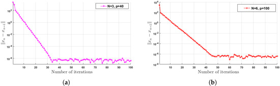
Figure 1. Algorithm 1 for different N and different dimensions $p=q$.

We now compare our algorithm for different ${\theta }_n$, i.e., for non-inertial accelerated case (${\theta }_n=0$) and for inertial accelerated case (${\theta }_n\ne 0$). For the non-inertial accelerated case, we just simply take $\theta =0$, and, for the inertial accelerated case, we take a very small $\theta$ with $\theta \in (0,1)$ so that ${\theta }_n={\overline{\theta }}_n=\theta$. Numerical comparisons of our proposed algorithm with inertial version (${\theta }_n\ne 0$) and its non-inertial version (${\theta }_n=0$) are presented in Table 3.

Table 3. Performance of Algorithm 1 for for different dimensions ${\theta }_n$, $N=3$ with $TOL={10}^{-3}$.

	$\mathit{P}=4$			$\mathit{P}=20$
	Iter(n)	CPU(s)	${\mathit{err}}_{\left(\mathit{n}\right)}$	Iter(n)	CPU(s)	${\mathit{err}}_{\left(\mathit{n}\right)}$
$\theta =0.1$	12	0.0811	0.3295	19	0.1005	0.4401
$\theta =0.01$	11	0.0844	0.3112	17	0.0968	0.3224
$\theta =0$	16	0.0960	0.5255	24	0.1203	0.4362

Remark 2.

Table 1 and Table 2 show that the CPU time and number of iterations of the algorithm increase linearly with the size or complexity of the problem (with the size of dimension p and q, number of mappings R and N, and number of functions M). From Table 3, we can see that our algorithm has a better performance for the stepsize choice ${\theta }_n\ne 0$. This implies that the inertial version of our algorithm has a better convergence analysis.

6. Conclusions

In this paper, we have proposed the problem of minimizing a convex function over the solution set of the split feasiblity problem of fixed point problems of demimetric mappings and constrained minimization problems of nonsmooth convex functions. We have showed that this problem can be solved by proximal and gradient methods where the gradient method is used for an upper level problem and the proximal method is used for a lower level problem. Most of the standard bilevel problems are particular cases of our framework.

References

- Su, M.; Xu, H.K. Remarks on the gradient-projection algorithm. J. Nonlinear Anal. Optim. 2010, 1, 35–43. [Google Scholar]
- Xu, H.K. Averaged mappings and the gradient-projection algorithm. J. Optim. Theory Appl. 2011, 150, 360–378. [Google Scholar] [CrossRef]
- Ceng, L.C.; Ansari, Q.H.; Yao, J.C. Some iterative methods for finding fixed points and for solving constrained convex minimization problems. Nonlinear Anal. Theor. 2011, 74, 5286–5302. [Google Scholar] [CrossRef]
- Rockafellar, R.T.; Wets, R.J. Variational Analysis; Springer Science & Business Media: Berlin, Germany, 2009. [Google Scholar]
- Bauschke, H.H.; Combettes, P.L. Convex Analysis and Monotone Operator Theory in Hilbert Spaces; Springer: New York, NY, USA, 2011. [Google Scholar]
- Martinet, B. Brève communication. Régularisation d’inéquations variationnelles par approximations successives. Revue Française d’Informatique et de Recherche Opérationnelle Série Rouge 1970, 4, 154–158. [Google Scholar] [CrossRef]
- Martinet, B. Détermination approchée d’un point fixe d’une application pseudo-contractante. CR Acad. Sci. Paris 1972, 274, 163–165. [Google Scholar]
- Rockafellar, R.T. Monotone operators and the proximal point algorithm. SIAM J. Control Optim. 1976, 14, 877–898. [Google Scholar] [CrossRef]
- Censor, Y.; Gibali, A.; Reich, S. Algorithms for the split variational inequality problem. Numer. Algorithms 2012, 59, 301–323. [Google Scholar] [CrossRef]
- Hendrickx, J.M.; Olshevsky, A. Matrix p-Norms Are NP-Hard to Approximate If p ≠ 1,2,∞. SIAM J. Matrix Anal. A 2010, 31, 2802–2812. [Google Scholar] [CrossRef]
- Censor, Y.; Elfving, T. A multiprojection algorithm using Bregman projections in a product space. Numer. Algorithms 1994, 8, 221–239. [Google Scholar] [CrossRef]
- Qu, B.; Xiu, N. A note on the CQ algorithm for the split feasibility problem. Inverse Probl. 2005, 21, 1655. [Google Scholar] [CrossRef]
- Byrne, C. Iterative oblique projection onto convex sets and the split feasibility problem. Inverse Probl. 2002, 18, 441. [Google Scholar] [CrossRef]
- López, G.; Martín-Márquez, V.; Wang, F.; Xu, H.K. Solving the split feasibility problem without prior knowledge of matrix norms. Inverse Probl. 2012, 28, 085004. [Google Scholar] [CrossRef]
- Yimer, S.E.; Kumam, P.; Gebrie, A.G.; Wangkeeree, R. Inertial Method for Bilevel Variational Inequality Problems with Fixed Point and Minimizer Point Constraints. Mathematics 2019, 7, 841. [Google Scholar] [CrossRef]
- Dempe, S.; Kalashnikov, V.; Pérez-Valdés, G.A.; Kalashnykova, N. Bilevel programming problems. In Energy Systems; Springer: Berlin, Germany, 2015. [Google Scholar]
- Anh, T.V. Linesearch methods for bilevel split pseudomonotone variational inequality problems. Numer. Algorithms 2019, 81, 1067–1087. [Google Scholar] [CrossRef]
- Anh, T.V.; Muu, L.D. A projection-fixed point method for a class of bilevel variational inequalities with split fixed point constraints. Optimization 2016, 65, 1229–1243. [Google Scholar] [CrossRef]
- Yuying, T.; Van Dinh, B.; Plubtieng, S. Extragradient subgradient methods for solving bilevel equilibrium problems. J. Inequal. Appl. 2018. [Google Scholar] [CrossRef]
- Shehu, Y.; Vuong, P.T.; Zemkoho, A. An inertial extrapolation method for convex simple bilevel optimization. Optim. Method Softw. 2019. [Google Scholar] [CrossRef]
- Sabach, S.; Shtern, S. A first order method for solving convex bilevel optimization problems. SIAM J. Optimiz. 2017, 27, 640–660. [Google Scholar] [CrossRef]
- Boţ, R.I.; Csetnek, E.R.; Nimana, N. An inertial proximal-gradient penalization scheme for constrained convex optimization problems. Vietnam J. Math. 2018, 46, 53–71. [Google Scholar] [CrossRef]
- Solodov, M. An explicit descent method for bilevel convex optimization. J. Convex Anal. 2007, 14, 227. [Google Scholar]
- Chang, S.S.; Quan, J.; Liu, J. Feasible iterative algorithms and strong convergence theorems for bi-level fixed point problems. J. Nonlinear Sci. Appl. 2016, 9, 1515–1528. [Google Scholar] [CrossRef][Green Version]
- Didi-Biha, M.; Marcotte, P.; Savard, G. Path-based formulations of a bilevel toll setting problem. In Optimization with Multivalued Mappings; Springer: Boston, MA, USA, 2006; pp. 29–50. [Google Scholar]
- Mohideen, M.J.; Perkins, J.D.; Pistikopoulos, E.N. Optimal design of dynamic systems under uncertainty. AIChE J. 1996, 42, 2251–2272. [Google Scholar] [CrossRef]
- Fampa, M.; Barroso, L.A.; Candal, D.; Simonetti, L. Bilevel optimization applied to strategic pricing in competitive electricity markets. Comput. Optim. Appl. 2008, 39, 121–142. [Google Scholar] [CrossRef]
- Calvete, H.I.; Galé, C.; Oliveros, M.J. Bilevel model for production–distribution planning solved by using ant colony optimization. Comput. Oper. Res. 2011, 38, 320–327. [Google Scholar] [CrossRef]
- Takahashi, S.; Takahashi, W. The split common null point problem and the shrinking projection method in Banach spaces. Optimization 2016, 65, 281–287. [Google Scholar] [CrossRef]
- Song, Y. Iterative methods for fixed point problems and generalized split feasibility problems in Banach spaces. J. Nonlinear Sci. Appl. 2018, 11, 198–217. [Google Scholar] [CrossRef]
- Cabot, A. Proximal point algorithm controlled by a slowly vanishing term: Applications to hierarchical minimization. SIAM J. Optim. 2005, 15, 555–572. [Google Scholar] [CrossRef]
- Helou, E.S.; Simões, L.E. ϵ-subgradient algorithms for bilevel convex optimization. Inverse Probl. 2017, 33, 5. [Google Scholar] [CrossRef]
- Polyak, B.T. Some methods of speeding up the convergence of iteration methods. USSR Comput. Math. Math. Phys. 1964, 4, 1–7. [Google Scholar] [CrossRef]
- Lemaire, B. Which fixed point does the iteration method select? In Recent Advances in Optimization; Springer: Berlin/Heidelberg, Germany, 1997; pp. 154–167. [Google Scholar]
- Xu, H.K. Iterative algorithms for nonlinear operators. J. Lond. Math. Soc. 2002, 66, 240–256. [Google Scholar] [CrossRef]
- Maingé, P.E. Strong convergence of projected subgradient methods for nonsmooth and nonstrictly convex minimization. Set Valued Anal. 2008, 16, 899–912. [Google Scholar] [CrossRef]
- Combettes, P.L.; Hirstoaga, S.A. Equilibrium programming in Hilbert spaces. J. Nonlinear Convex Anal. 2005, 6, 117–136. [Google Scholar]
- Aubin, J.P. Optima and Equilibria: An Introduction to Nonlinear Analysis; Springer Science & Business Media: Berlin, Germany, 2013. [Google Scholar]
© 2020 by the authors. Licensee MDPI, Basel, Switzerland. This article is an open access article distributed under the terms and conditions of the Creative Commons Attribution (CC BY) license (http://creativecommons.org/licenses/by/4.0/).