Article

Taming Hyperchaos with Exact Spectral Derivative Discretization Finite Difference Discretization of a Conformable Fractional Derivative Financial System with Market Confidence and Ethics Risk

by
Dominic P. Clemence-Mkhope
* and
Gregory A. Gibson
Department of Mathematics and Statistics, North Carolina A&T State University, Greensboro, NC 27411, USA
*
Author to whom correspondence should be addressed.
Math. Comput. Appl. 2022, 27(1), 4; https://doi.org/10.3390/mca27010004
Submission received: 27 November 2021 / Revised: 29 December 2021 / Accepted: 31 December 2021 / Published: 10 January 2022

Abstract

:
Four discrete models, using the exact spectral derivative discretization finite difference (ESDDFD) method, are proposed for a chaotic five-dimensional, conformable fractional derivative financial system incorporating ethics and market confidence. Since the system considered was recently studied using the conformable Euler finite difference (CEFD) method and found to be hyperchaotic, and the CEFD method was recently shown to be valid only at fractional index α = 1 , the source of the hyperchaos is in question. Through numerical experiments, illustration is presented that the hyperchaos previously detected is, in part, an artifact of the CEFD method, as it is absent from the ESDDFD models.

1. Introduction

Hyperchaotic systems [1,2]—typically defined as systems with at least two positive Lyapunov exponents [3,4,5]—of a fractional-order have been investigated in many contexts, such as systems of Rössler [6] or Lorenz [7] type, those with flux controlled memristors [8] or realized in circuits [9,10,11], those arising from cellular neural networks [12], and financial systems [13]. As recounted in [13], a nonlinear financial system depicting the relationship among interest rates, investments, prices, and savings was first introduced by Huang and Li [14]. It was extended to fractional-order in Chen [15], to uncertain fractional-order form in Wang et al. [16], to delayed form in Mircea et al. [17], and to discrete form in Xin et al. [18]. The average profit margin was added as a variable in Yu et al. [19], while investment incentive and market confidence were introduced in Xin et al. [20,21]. Xin and Zhang [21] updated the 3-dimensional Huang and Li [8] model to a 4-dimensional one by accounting for market confidence and [13] incorporated ethics risk to obtain a 5-dimensional system, which was then fractionalized to obtain the following fractional-order financial system considered in [13]:
T t α 1 x = z + ( y a ) x + k ( w p u ) T t α 2 y = 1 b y x 2 + k ( w p u ) T t α 3 z = x c z + k ( w p u ) T t α 4 w = d x y z T t α 5 u = k ( w p u )
where α = ( α 1 , α 2 , α 3 , α 4 , α 5 ) is subject to α 1 , α 2 , α 3 , α 4 , α 5 ( 0 ,   1 ) , and T t α i , 1 i 5 , denotes the conformable fractional derivative of order α i . The variables x, y, z, w, and u are the interest rate, investment demand, price index, market confidence, and ethics risk, respectively; the parameters a, b, and c are the saving amount, cost per investment, and demand elasticity of commercial markets, respectively, and a, b, c ≥ 0; k, p, d are impact factors associated with ethics risk.
Since analytic solutions do not exist, suitable numerical schemes to obtain solutions of the conformable derivative financial system are needed. Though there are several methods to solve a conformable derivative system [22,23,24,25,26,27,28,29,30,31,32,33,34,35,36,37,38,39,40,41,42,43,44,45,46,47], these are too complex for many people. Inspired by the discretization process for the Caputo derivative for Ricatti equations [45] and Chua systems [46], the conformable Euler’s finite difference (CEFD) method [47] for the 5-dimensional fractional-order financial system is proposed in [13]. Numerical experiments with the resulting discrete model were conducted to detect a hyperchaotic attractor of the system. However, the standard Euler discretization of integer-order systems, such as studied in [13], is known to induce (see, e.g., [48,49]) numerical instabilities and spurious behavior where none exist in the continuous system. Moreover, the CEFD method has recently been shown [50] to be valid only for α = 1 and is, therefore, not a valid fractional method. Nonstandard finite difference (NSFD) models have extensively [48] been shown to eliminate induced chaos; the exact spectral derivative discretization finite difference (ESDDFD) methodology is a novel extension, developed in the context of advection–reaction–diffusion equations [51], of the NSFD method to non-integer derivatives [52].
It is, therefore, natural to ask whether some of the hyperchaotic behavior detected in the fractional financial system is an artifact of the method and whether ESDDFD models can be constructed to eliminate such induced hyperchaos. The purpose of the present study is to investigate this question—in particular, the effects of the discretization of the derivative and that of non-linear terms. To this end, the following four discrete models using the ESDDFD method are constructed for the system (1) and the bifurcation experiments of [13] are repeated with the new models.
x k + 1 x k ϕ j ( h , α 1 ) = F i x ( x k , y k , z k , u k , w k ) y k + 1 y k ϕ j ( h , α 2 ) = F i y ( x k , y k , z k , u k , w k ) z k + 1 z k ϕ j ( h , α 3 ) = x k c z k + k ( w k p u k ) u k + 1 u k ϕ j ( h , α 5 ) = k ( w k p u k ) w k + 1 w k ϕ j ( h , α 4 ) = F i w ( x k , y k , z k , z k )
i = 1 ,   2 and j = 1 ,   2 , where:
F 1 x ( x k , y k , z k , u k , w k ) = z k + ( y k + 1 a ) x k + k ( w k p u k ) F 1 y ( x k , y k , z k , u k , w k ) = 1 b y k x k x k + k ( w k p u k ) F 1 w ( x k , y k , z k , z k ) = d 2 x k y k ( z k + z k ) F 2 x = F 1 x ( x k , y k + 1 , z k , u k , w k ) F 2 y = F 1 y ( x k , y k + 1 , z k , u k , w k ) F 2 w = F 1 w ( x k , y k + 1 , z k , z k + 1 )
The remainder of this article is organized as follows. In Section 2, the ESDDFD fundamentals, a description of the model (1), and the CEFD model from [3] are presented. Section 3 presents the construction of the denominator functions, ϕ j ( h , α m ) , 1 m 5 , for the ESDDFD model (2) and compares sub-models of (2) with corresponding CEFD sub-models. In Section 4, experimental results of hyperchaotic attractor detection from the proposed financial system using both methods are presented. Concluding remarks in Section 5 close the paper.

2. Preliminaries

2.1. The Conformable Derivative ESDDFD Discrete Model Construction Fundamentals

While the Riemann–Liouville, Caputo, Atangana–Baleanu, and Grünwald–Letnikov fractional derivatives [53,54,55,56,57,58,59,60] are widely used in various applications, their definitions lack the chain rule, a classical derivative property satisfied by the conformable fractional derivative (CFD) [61,62,63] and its various extensions (see e.g., [64]). A financial system with a market confidence and ethics risk model was recently [13] added to the many existing applications of the CFD in various scientific fields [22,65,66,67,68,69,70,71,72,73,74].

2.2. The Conformable Derivative Hyperchaotic Financial System and Its CEFD Model

The conformable fractional derivative financial system model (1) is based on a successive addition of various factors, starting with the Huang and Li [8] nonlinear financial system model:
x = z + ( y a ) x y = 1 b y x 2 z = x c z
modeling the interaction of interest rate ( x ), investment demand ( y ) , and price index ( z ) ; the variables and parameters are the same as in (1). Model (3) was extended, by Xin and Zhang [15], to account for market confidence:
x = z + ( y a ) x + m 1 w y = 1 b y x 2 + m 2 w z = x c z + m 3 w w = d x y z
where m 1 , m 2 , m 3 are the impact factors associated with market confidence ( w ) ; the remaining variables and parameters are the same as in (3). Model (1) is the fractionalization, predicated on the practice that fractional-order economic systems [15,75,76,77,78,79] can generalize their integer-order forms [14,80,81], of the following extension of (4) in [13] to account for both market confidence and ethics risk ( u ) :
x = z + ( y a ) x + k ( w p u ) y = 1 b y x 2 + k ( w p u ) z = x c z + k ( w p u ) w = d x y z u = k ( w p u )
When α = (1, 1, 1, 1, 1), system (1) degenerates to system (5); in the absence of ethics risk, (5) reduces to (4); in the absence of market confidence, (4) reduces to (3). In these three cases, therefore, any discrete method developed for (1) must reduce to that of the three respective reduced systems. Chaotic behavior for both the CEFD and ESDDFD models will be numerically investigated in Section 4 for (1) as well as the reduced fractional counterpart of system (3).
The following discrete model was obtained in [13] from the CEFD method and used to numerically investigate hyperchaos of the system (1):
x k + 1 = x k + h α 1 α 1 ( z k + ( y k a ) x k + k ( w k p u k ) ) y k + 1 = y k + h α 2 α 2 ( 1 b y k x k x k + k ( w k p u k ) ) z k + 1 = z k h α 3 α 3 ( x k + c z k k ( w k p u k ) ) u k + 1 = u k + h α 5 α 5 k ( w k p u k ) w k + 1 = w k h α 4 α 4 d x k y k z k

3. ESDDFD Discretization of the Conformable Derivative System and Its Reductions

In the ESDDFD and NSFD discretization methodologies, the first step is to consider a linear sub-system whose exact or best scheme can be constructed. Such a sub-system, in this case, is the following:
T t α 1 x = a x , T t α 2 y = b y , T t α 3 z = c z , T t α 4 w = 0 , T t α 5 u = k p u ,
which has only positive solutions for any positive initial data. The exact discretization of (7), which has a solution identical to that of (7), is as follows:
x k + 1 x k ϕ 1 ( h , α 1 ) = a x k , y k + 1 y k ϕ 1 ( h , α 2 ) = b y k , z k + 1 z k ϕ 1 ( h , α 3 ) = c z k , w k + 1 w k ϕ 1 ( h , α 4 ) = 0 , u k + 1 u k ϕ 1 ( h , α 5 ) = k p u k ,
where the nonstandard denominators ϕ 1 ( h , α i ) , 1 i 5 ,   are given by:
ϕ 1 ( h , α i ) = 1 Q i ( 1 e Q i α i [ ( t + h ) α i t α i ] ) ,   with   Q 1 = a ,   Q 2 = b ,   Q 3 = c ,   Q 4 = 0 ,   Q 5 = k p .
Since (1) reduces to (7), any valid discrete model for (1) must be reducible to one consistent with its exact discretization—that is, (8). By comparison, a reduction of the CEFD model (6) to the sub-system (7) yields the following discrete sub-system:
x k + 1 = x k h α 1 α 1 a x k , y k + 1 = y k h α 2 α 2 b y k , z k + 1 = z k h α 3 α 3 c z k , w k + 1 = w k + Q 4 h α 4 α 4 w k , u k + 1 = u k h α 5 α 5 k p u k ,
which is positive only if the following condition is satisfied: ( 1 h α i α i Q i ) 0 ,   1 i 5 , with the Q i as in (8); such conditional positivity is known to induce chaotic behavior. All of the sub-Equations (8) are of the form:
T t α P = λ P ,
whose CEFD scheme is:
P k + 1 = P k h α α λ P k ,
which has been conclusively shown in [50] to be valid only for α = 1 .
It is shown in [50] that a modified CEFD (MCEFD) may be obtained from the following alternate CFD definition, which is equivalent to the fractional change of variables in the integer-valued derivative (see also [82]):
Definition 1.
Given a real-valued function on [ 0 , ) , the conformable fractional derivative has the following alternative definition:
T 0 C t α [ f ( t ) ] lim h 0 0 C F D t α [ f ( t ) ] = α lim h 0 f ( t + h ) f ( t ) [ ( t + h ) α t α ]   ,
where  T 0 C t α [ f ( 0 ) ] isunderstood to mean  T 0 C t α [ f ( 0 ) ] = lim t 0 + T 0 C t α [ f ( t ) ] .
Therefore, the Euler scheme, resulting from the MCFED, is the same as that given in Equation (8), only with the denominator of:
ϕ 1 ( h , α i ) = 1 Q i ( 1 e Q i α i [ ( t + h ) α i t α i ] )
replaced by:
ϕ 2 ( h , α i ) = 1 α i [ ( t + h ) α i t α i ] ,   1 i 5 ,
which is equivalent to replacing h α i by α i ϕ 2 ( h , α i ) in the CEFD scheme (9).
To enable the assessment of the effect of the denominators ϕ j ( h , α i ) ,   j = 1 , 2 , the following schemes are compared:
x k + 1 x k ϕ j ( h , α 1 ) =   z k     + ( y k a ) x k   ,     y k + 1 y k ϕ j ( h , α 2 ) = 1 b y k ( x k ) 2 , z k + 1 z k ϕ j ( h , α 3 ) = x k c z k ,     j = 1 , 2 .
To enable the assessment of the effect of the non-local discretization of nonlinear terms, the following schemes are compared:
x k + 1 x k ϕ j ( h , α 1 ) = z k + ( y k + 1 a ) x k , y k + 1 y k ϕ j ( h , α 2 ) = 1 b y k x k + 1 x k , z k + 1 z k ϕ j ( h , α 3 ) = x k c z k ,     j = 1 ,   2 .
The terms ( y a ) x , and x 2 are discretized non-locally as, respectively,   ( y k + 1 a ) x k and x k + 1 x k , while discretization of the terms z (in the first Equation of (10)) and x (in the third as z k and x k ) ensures respective consistency with the terms c z in the third and a x in the first Equation of (11) in the cases where c = 1 and a = 1 .
By comparison, the scheme obtained through a reduction of the CEFD model (6) to its 3-dimensional sub-system (3) yields the following discrete sub-system:
x k + 1 = x k + h α 1 α 1 ( z k + ( y k a ) x k ) y k + 1 = y k + h α 2 α 2 ( 1 b y k x k x k ) z k + 1 = z k + h α 3 α 3 ( x k c z k ) .
Since system (12) reduces to the x y z sub-system of (9), which suffers from induced chaos, it is to be expected that it too suffers the same, which will be numerically investigated in the next section.
The ESDDFD models (2) are then obtained by discretizing k ( w p u ) as k ( w k p u k ) to ensure consistency with (8) and then discretizing x y z non-locally as either 1 2 x k y k ( z k + z k ) or 1 2 x k y k + 1 ( z k + z k + 1 ) , where the form x k y k + 1 is used to match the x y term in the x -equation.
x k + 1 x k ϕ j ( h , α 1 ) = z k + ( y k a ) x k + k ( w k p u k ) y k + 1 y k ϕ j ( h , α 2 ) = 1 b y k ( x k ) 2 + k ( w k p u k ) z k + 1 z k ϕ j ( h , α 3 ) = x k c z k + k ( w k p u k ) u k + 1 u k ϕ j ( h , α 5 ) = k ( w k p u k ) w k + 1 w k ϕ j ( h , α 4 ) = d 2 x k y k ( z k + z k ) ,     j = 1 , 2 .
and
x k + 1 x k ϕ j ( h , α 1 ) = z k + ( y k + 1 a ) x k + k ( w k p u k ) y k + 1 y k ϕ j ( h , α 2 ) = 1 b y k x k + 1 x k + k ( w k p u k ) z k + 1 z k ϕ j ( h , α 3 ) = x k c z k + k ( w k p u k ) u k + 1 u k ϕ j ( h , α 5 ) = k ( w k p u k ) w k + 1 w k ϕ j ( h , α 4 ) = d 2 x k y k + 1 ( z k + z k + 1 ) ,     j = 1 , 2 .
The schemes (13) are explicit and can be explicitly solved for each j = 1 , 2 , in the order x k + 1 , y k + 1 , z k + 1 , u k + 1 , w k + 1 to obtain the following:
x k + 1 = x k + ϕ j ( h , α 1 ) [ z k + ( y k a ) x k + k ( w k p u k ) ] y k + 1 = y k + ϕ j ( h , α 2 ) [ 1 b y k ( x k ) 2 + k ( w k p u k ) ] z k + 1 = z k ϕ j ( h , α 3 ) [ x k + c z k k ( w k p u k ) ] u k + 1 = u k + ϕ j ( h , α 5 ) [ k ( w k p u k ) ] w k + 1 = w k d 2 ϕ j ( h , α 4 ) x k y k ( z k + z k ) ,     j = 1 , 2 .
While implicit, the schemes (14) can be explicitly solved for each j = 1 , 2 in the order u k + 1 , z k + 1 , x k + 1 , y k + 1 ,   w k + 1 to obtain the following:
u k + 1 = u k + ϕ j ( h , α 5 ) [ k ( w k p u k ) ] z k + 1 = z k ϕ j ( h , α 3 ) [ x k + c z k k ( w k p u k ) ] x k + 1 = 1 [ 1 + ϕ j ( h , α 1 ) x k ϕ j ( h , α 2 ) x k ] ( x k + ϕ j ( h , α 1 ) x k { y k + ϕ j ( h , α 2 ) [ 1 b y k + k ( w k p u k ) ] } ) + 1 [ 1 + ϕ ( h , α 1 ) x k ϕ ( h , α 2 ) x k ] ϕ j ( h , α 1 ) [ z k a x k + k ( w k p u k ) ] w k + 1 = w k ϕ j ( h , α 4 ) d 2 x k y k + 1 ( z k + z k + 1 )

4. Numerical Experiments

In this section, hyperchaos detection experiments are conducted, parallel to those of [13], by varying the parameters related to ethics risk, such as α 5 , the confidence factor k, and the risk factor p, in the CEFD and ESDDFD models and their reductions. The following parameters and initial point values are fixed following [1]: h = 0.002 ,   a = 0.8 ,   b = 0.6 ,   c = 1 ,   d = 2 ,   α 1 = 0.3 ,   α 2 = 0.5 ,   α 3 = 0.6 ,   α 4 = 0.24 ,   x 0 = 0.4 ,   y 0 = 0.6 ,   z 0 = 0.8 ,   w 0 = 0.3 ,   u 0 = 0.4 .

4.1. Three-Dimensional Systems Comparison

There were no experiments performed in [13] for this case. Simulations for both the ESDDFD model (11) and the CEFD model (12) are performed with the same parameters. The following models (16)–(19), obtained through the ESDDFD method,
x k + 1 x k 1 0.8 [ 1 e 0.8 0.3 [ ( t + h ) 0.3 t 0.3 ] ] = z k + ( y k 0.8 ) x k , y k + 1 y k 1 0.6 [ 1 e 0.6 0.5 [ ( t + h ) 0.5 t 0.5 ] ] = 1 0.6 y k ( x k ) 2 , z k + 1 z k [ 1 e 1 0.6 [ ( t + h ) 0.6 t 0.6 ] ] = x k z k ,
x k + 1 x k 1 0.3 [ ( t + h ) 0.3 t 0.3 ] = z k + ( y k 0.8 ) x k , y k + 1 y k 1 0.5 [ ( t + h ) 0.5 t 0.5 ] = 1 0.6 y k ( x k ) 2 , z k + 1 z k 1 0.6 [ ( t + h ) 0.6 t 0.6 ] = x k z k ,
x k + 1 x k 1 0.8 [ 1 e 0.8 0.3 [ ( t + h ) 0.3 t 0.3 ] ] = z k + ( y k + 1 0.8 ) x k , y k + 1 y k 1 0.6 [ 1 e 0.6 0.5 [ ( t + h ) 0.5 t 0.5 ] ] = 1 0.6 y k x k + 1 x k , z k + 1 z k [ 1 e 1 0.6 [ ( t + h ) 0.6 t 0.6 ] ] = x k z k ,
x k + 1 x k 1 0.3 [ ( t + h ) 0.3 t 0.3 ] = z k + ( y k + 1 0.8 ) x k , y k + 1 y k 1 0.5 [ ( t + h ) 0.5 t 0.5 ] = 1 0.6 y k x k + 1 x k , z k + 1 z k 1 0.6 [ ( t + h ) 0.6 t 0.6 ] = x k
are compared to (20), obtained through the CEFD method:
x k + 1 x k + h 0.3 0.3 ( z k + ( y k 0.8 ) x k ) , y k + 1 = y k + h 0.5 0.5 ( 1 0.6 y k x k x k ) , z k + 1 = z k + h 0.6 0.6 ( x k z k ) .
While bifurcations can be seen in Figure 1a for the CEFD model, they are absent from the results of the ESDDFD models, Figure 1b–e.

4.2. Five-Dimensional Systems Comparison: Varying α 5 ,   k , and p

For this case, experiments performed in [13] are performed with the same parameters for models obtained through the ESDDFD method, for the various cases and values of ( α 5 ,   k ,   p ) used in [13]. Model (21) from the CEFD method,
x k + 1 = x k + h 0.3 0.3 ( z k + ( y k 0.8 ) x k + k ( w k p u k ) ) y k + 1 = y k + h 0.5 05 ( 1 0.6 y k x k x k + k ( w k p u k ) ) z k + 1 = z k h 0.6 0.6 ( x k + z k k ( w k p u k ) ) w k + 1 = w k h 0.24 0.24 2 x k y k z k u k + 1 = u k + h α 5 α 5 k ( w k p u k )
is compared to the following four models—respectively, MCEFD (22), ESDDFD1 (23), ESDDFD2 (24), ESDDFD3 (25)—obtained through the ESDDFD and NSFD methods:
x k + 1 x k 1 0.3 [ ( t + h ) 0.3 t 0.3 ] = z k + ( y k 0.8 ) x k + k ( w k p u k ) y k + 1 y k 1 0.5 [ ( t + h ) 0.5 t 0.5 ] = 1 0.6 y k x k x k + k ( w k p u k ) z k + 1 z k 1 0.6 [ ( t + h ) 0.6 t 0.6 ] = x k z k + k ( w k p u k ) w k + 1 w k 1 0.24 [ ( t + h ) 0.24 t 0.24 ] = x k y k ( z k + z k ) u k + 1 u k 1 α 5 [ ( t + h ) α 5 t α 5 ] = k ( w k p u k )
x k + 1 x k 1 0.8 [ 1 e 0.8 0.3 [ ( t + h ) 0.3 t 0.3 ] ] = z k + ( y k 0.8 ) x k + k ( w k p u k ) y k + 1 y k 1 0.6 [ 1 e 0.6 0.5 [ ( t + h ) 0.5 t 0.5 ] ] = 1 0.6 y k x k x k + k ( w k p u k ) z k + 1 z k [ 1 e 1 0.6 [ ( t + h ) 0.6 t 0.6 ] ] = x k z k + k ( w k p u k ) w k + 1 w k [ 1 e 1 0.24 [ ( t + h ) 0.24 t 0.24 ] ] = x k y k ( z k + z k ) u k + 1 u k 1 kp [ 1 e k p α 5 [ ( t + h ) α 5 t α 5 ] ] = k ( w k p u k )
x k + 1 x k 1 0.3 [ ( t + h ) 0.3 t 0.3 ] = z k + ( y k + 1 0.8 ) x k + k ( w k p u k ) y k + 1 y k 1 0.5 [ ( t + h ) 0.5 t 0.5 ] = 1 0.6 y k x k + 1 x k + k ( w k p u k ) z k + 1 z k 1 0.6 [ ( t + h ) 0.6 t 0.6 ] = x k z k + k ( w k p u k ) w k + 1 w k 1 0.24 [ ( t + h ) 0.24 t 0.24 ] = x k y k + 1 ( z k + z k + 1 ) u k + 1 u k 1 α 5 [ ( t + h ) α 5 t α 5 ] = k ( w k p u k )
x k + 1 x k 1 0.8 [ 1 e 0.8 0.3 [ ( t + h ) 0.3 t 0.3 ] ] = z k + ( y k + 1 0.8 ) x k + k ( w k p u k ) y k + 1 y k 1 0.6 [ 1 e 0.6 0.5 [ ( t + h ) 0.5 t 0.5 ] ] = 1 0.6 y k x k + 1 x k + k ( w k p u k ) z k + 1 z k [ 1 e 1 0.6 [ ( t + h ) 0.6 t 0.6 ] ] = x k z k + k ( w k p u k ) w k + 1 w k [ 1 e 1 0.24 [ ( t + h ) 0.24 t 0.24 ] ] = x k y k + 1 ( z k + z k + 1 ) u k + 1 u k 1 kp [ 1 e k p α 5 [ ( t + h ) α 5 t α 5 ] ] = k ( w k p u k )

4.2.1. Varying α5 with Fixed k = 2 and p = 1 and α5 ∈ [0.232, 0.328]

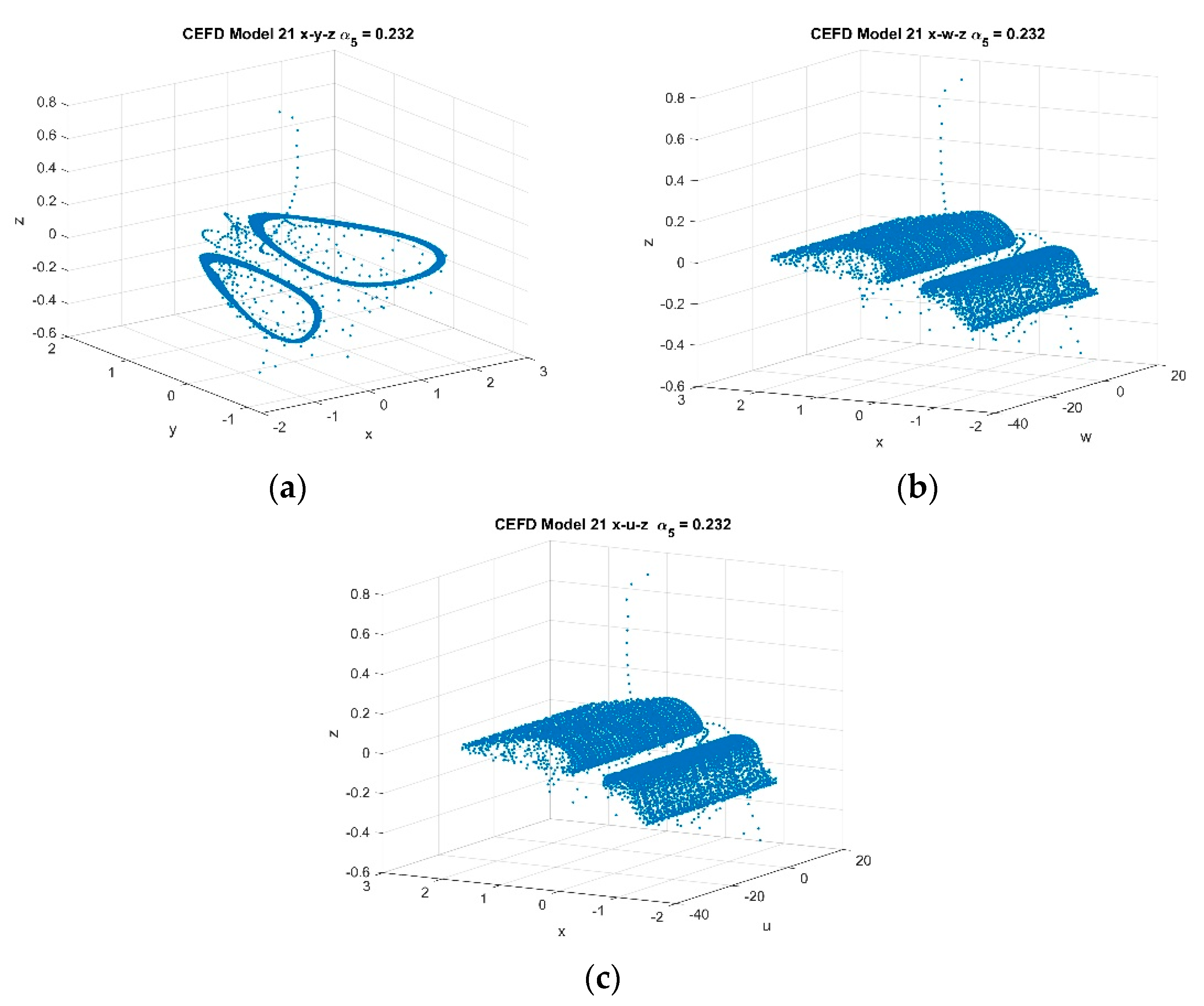
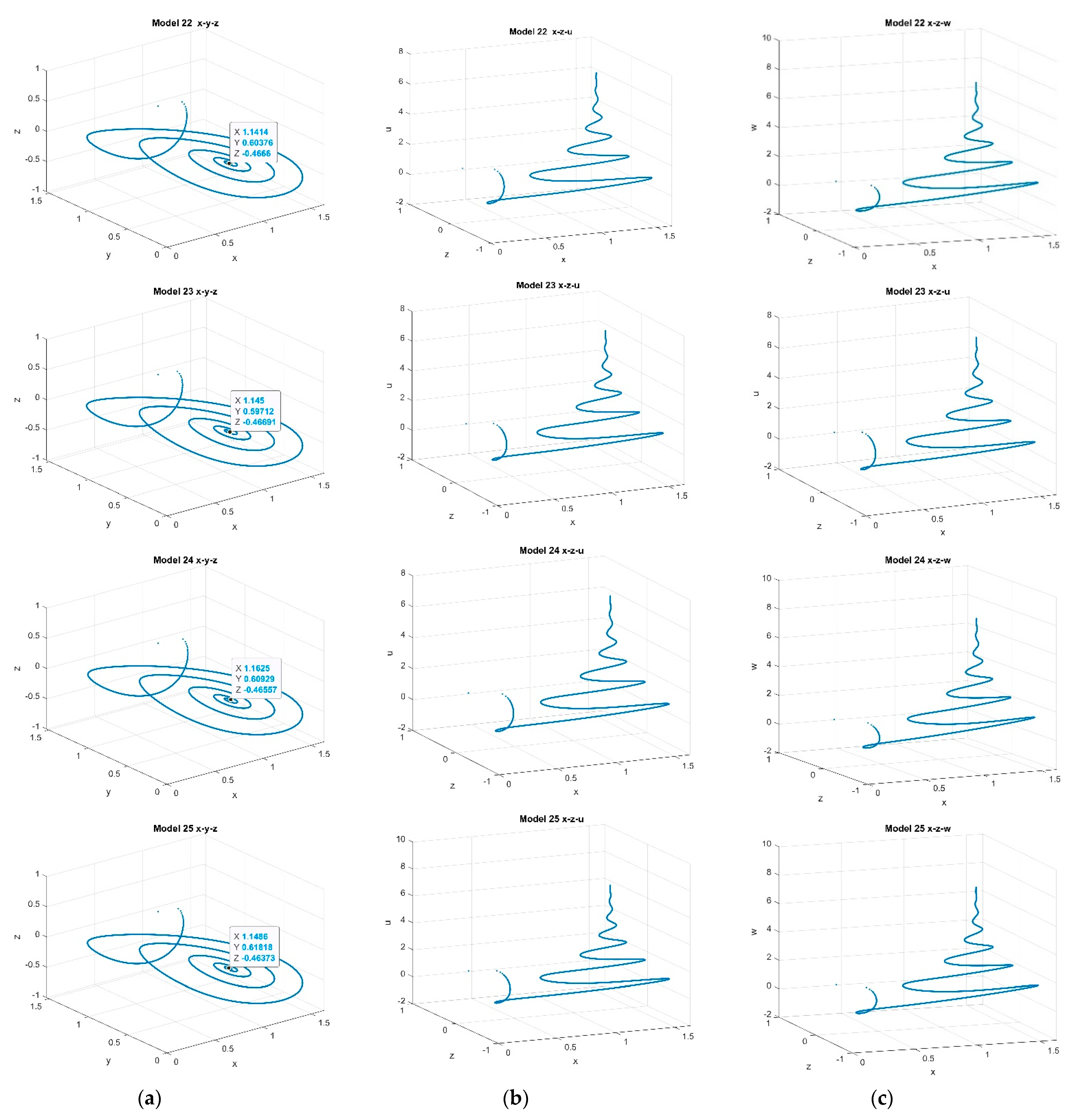
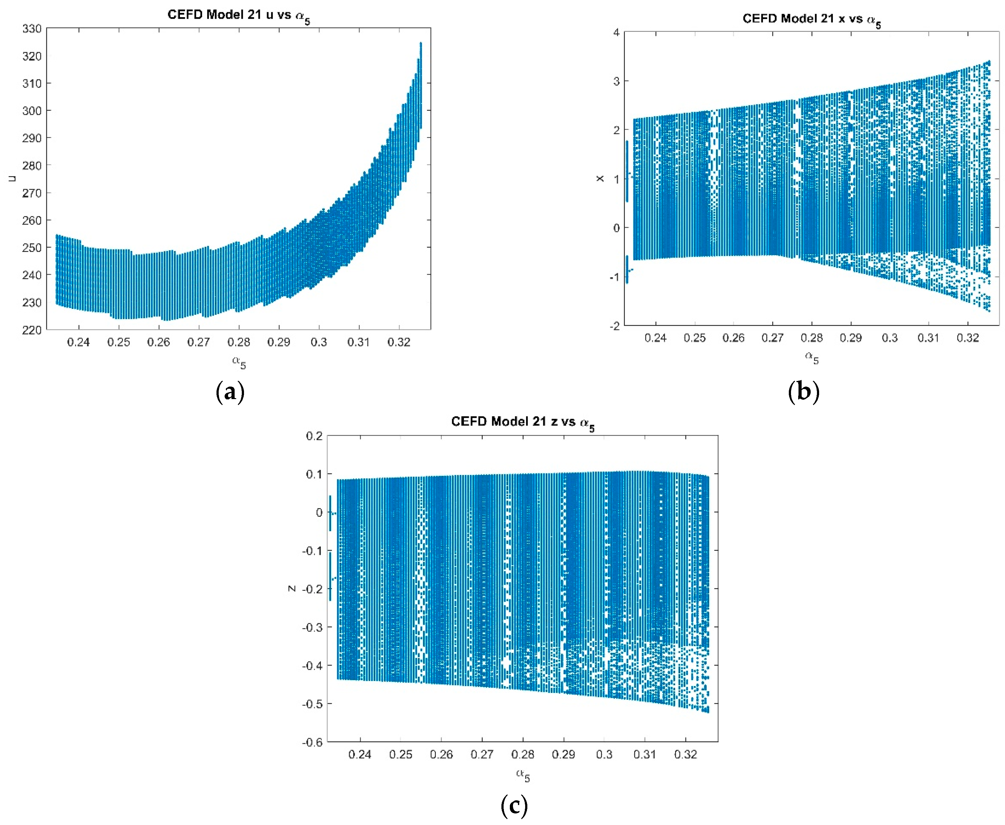
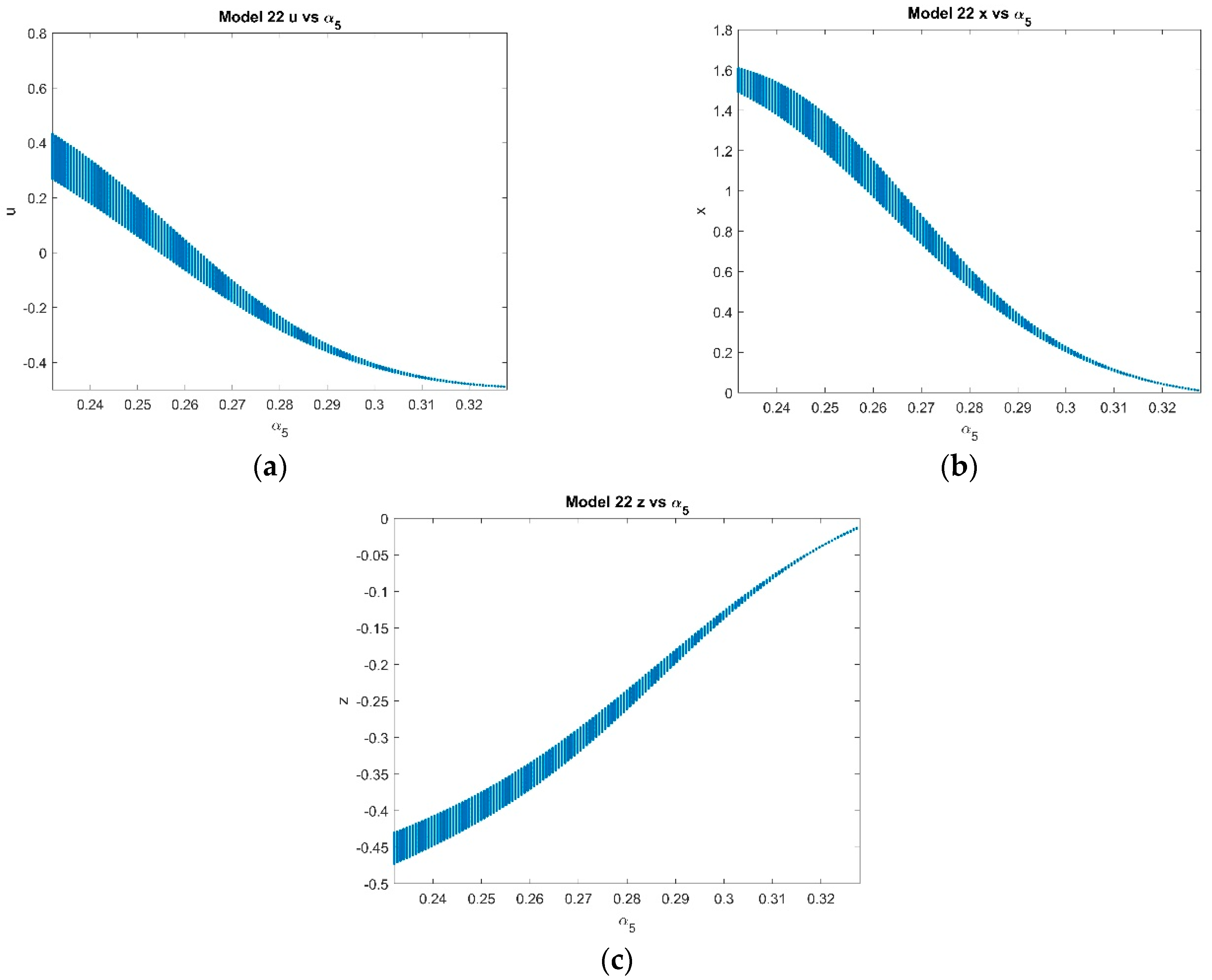
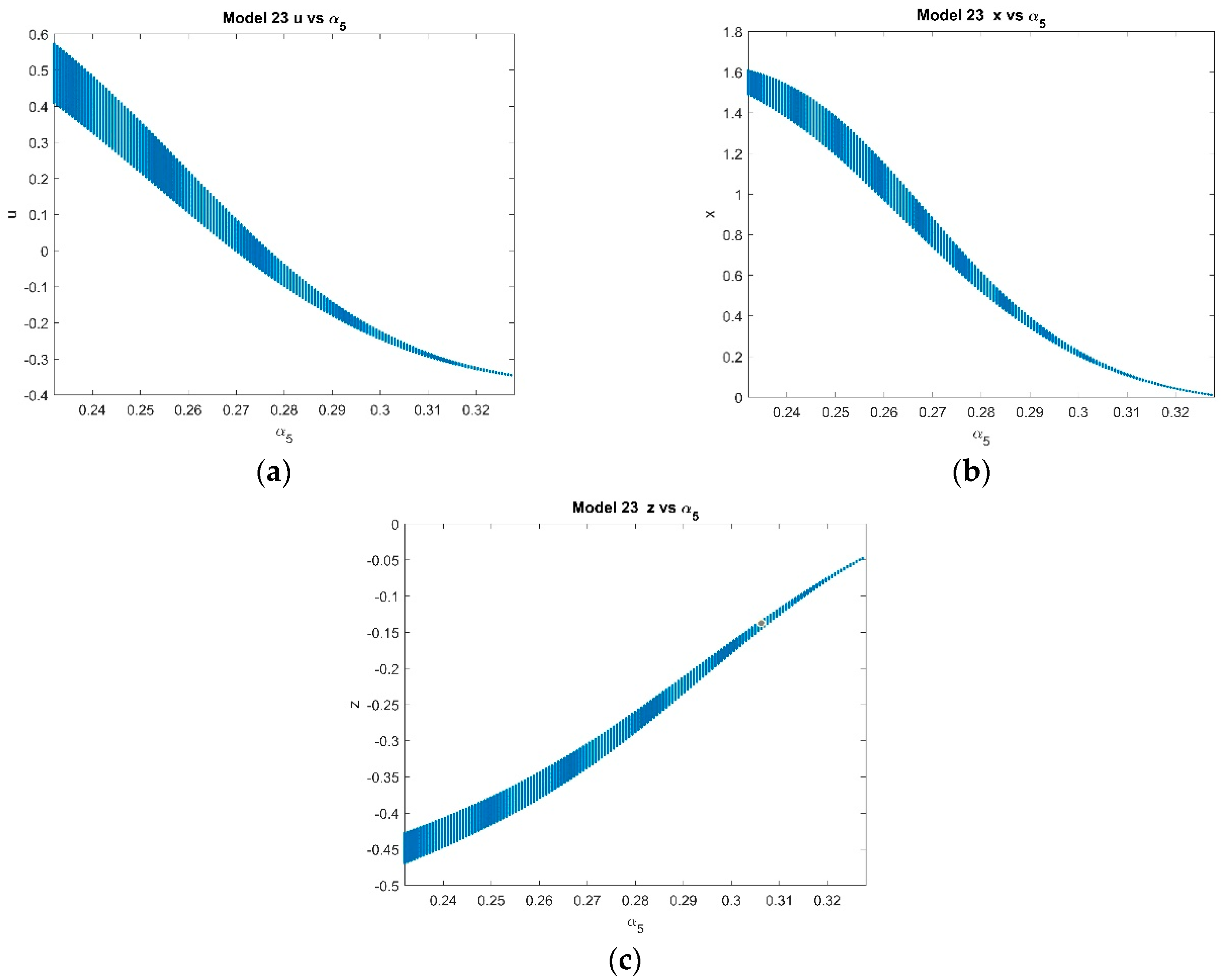
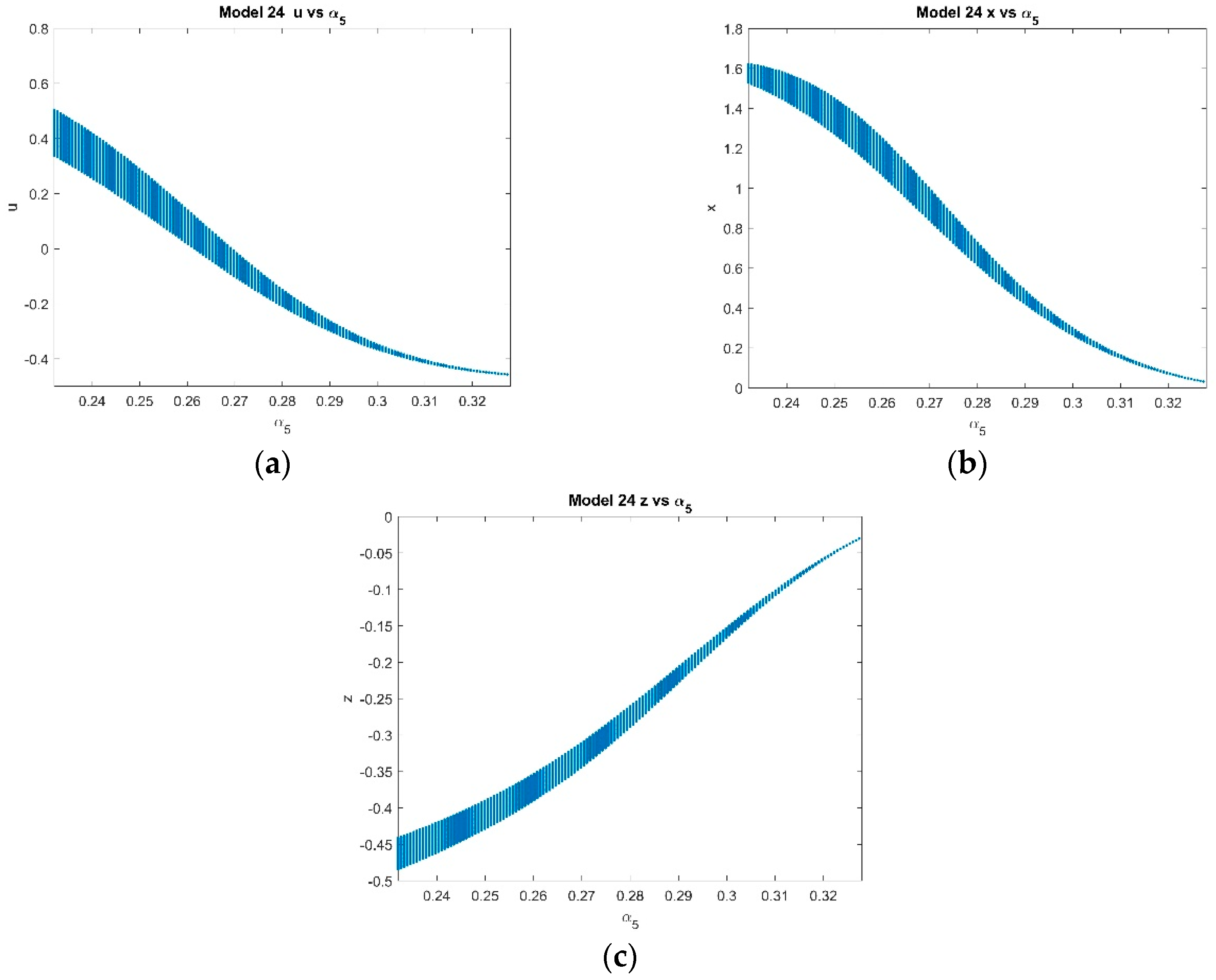
In this case, Ref. [13] concluded that system (6) is hyperchaotic with α5 ∈ [0.232, 0.328]; fixing α 5 = 0.24 , a set of two positive Lyapunov exponents and three negative Lyapunov exponents were found. Profiles for x ,   y ,   z ,   w and u , when α 5 = 0.232 for model (21), are given below. Chaos can be clearly seen in Figure 2 which gives the phase portraits for the CEFD model. For each model (22) through (25). Figure 3 shows phase portraits using the same step size and parameter values. These models produce identical graphs, which differ significantly from the graphs for model (21). The bifurcation tests for the ESDDFD model are performed with the same parameters. The bifurcation diagrams for x , z   and u for model (21) are in Figure 4. These again show clear signs of chaos while the bifurcation diagrams for models (22) through (25), which are given in Figure 5, Figure 6, Figure 7 and Figure 8, do not.
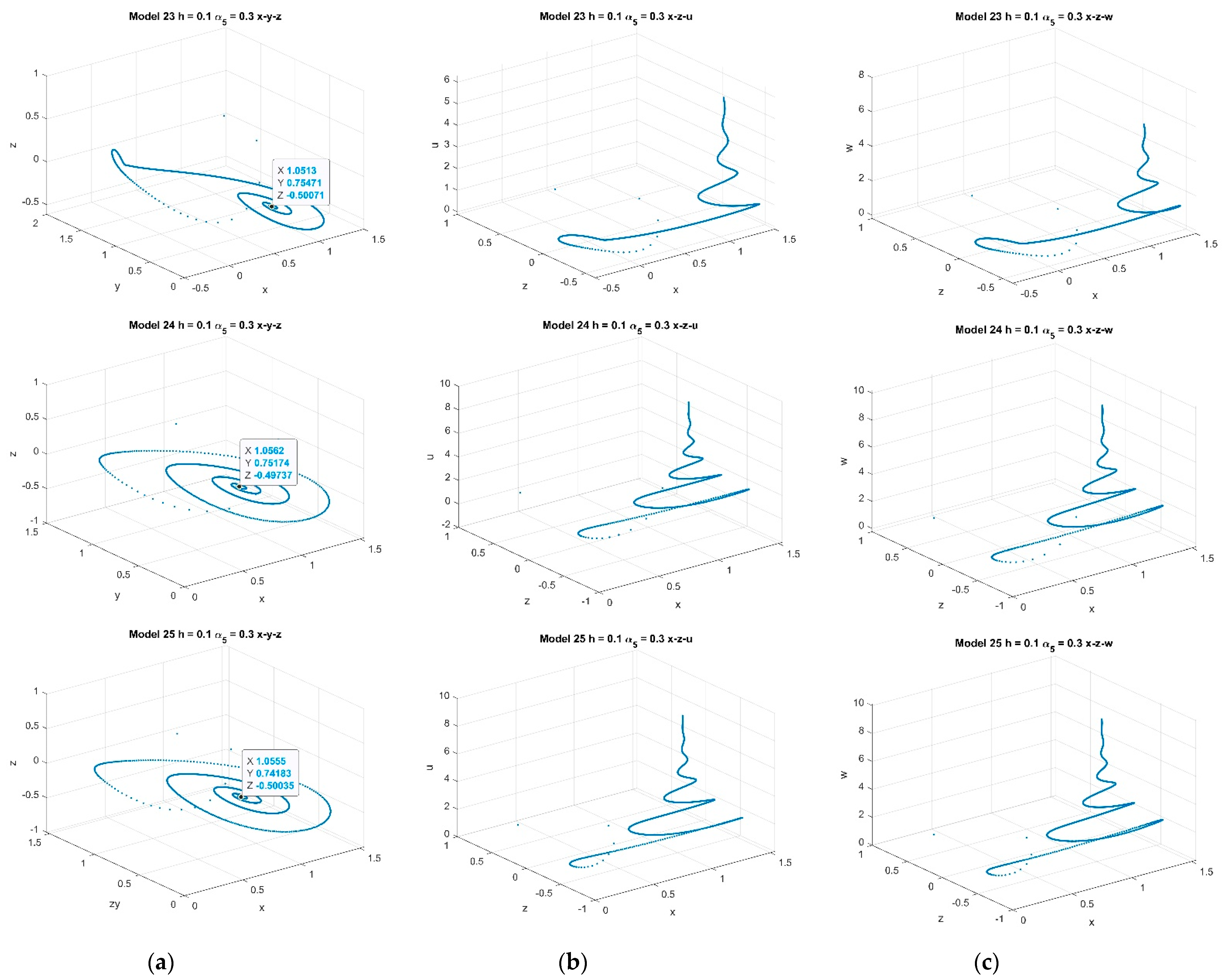
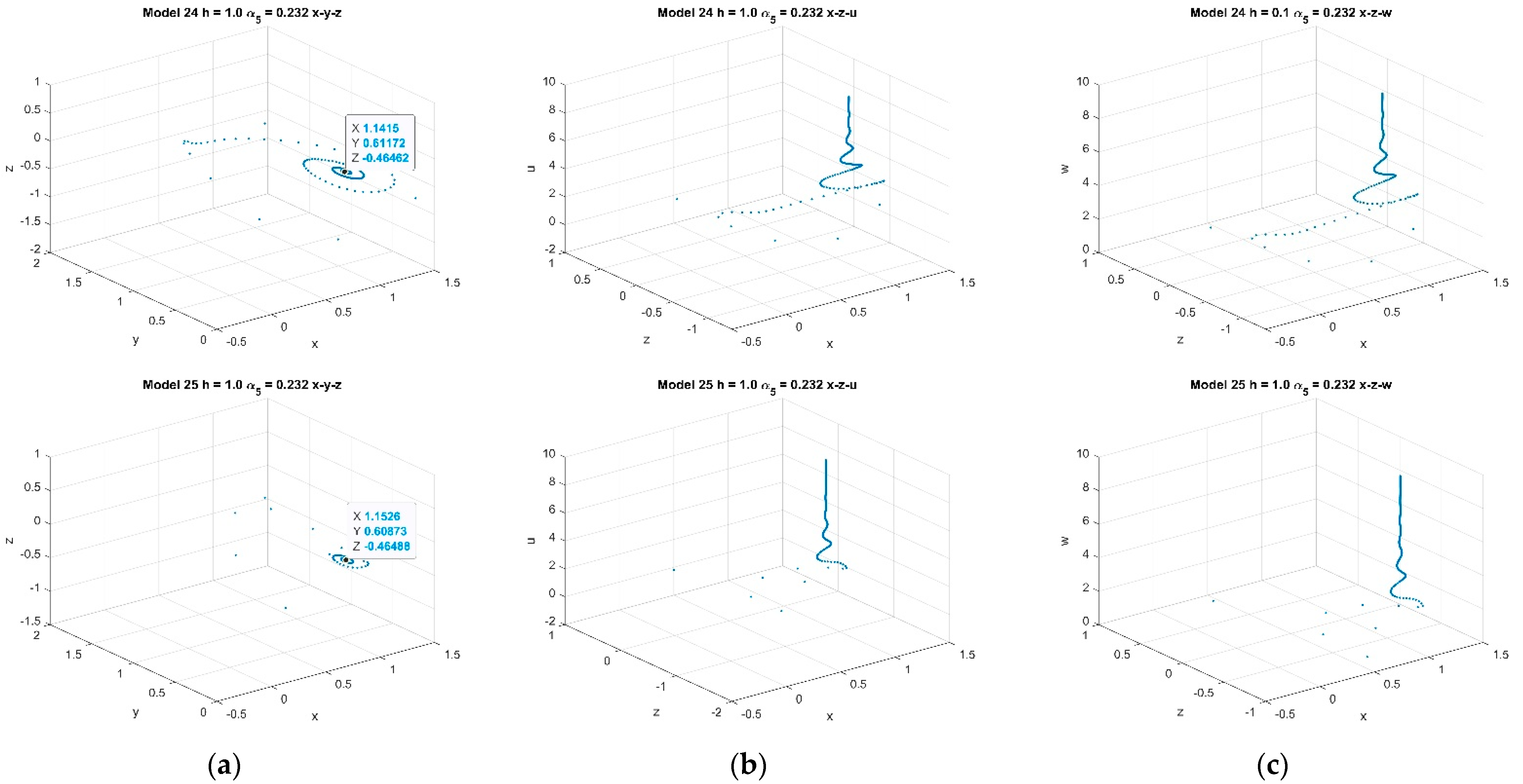
For step sizes above 0.003, CEFD, (21), fails. MCEFD, (22) fails for step sizes above 0.573. The graphs in Figure 9 were produced using the same parameter values as before, except h = 0.1 . The graphs in Figure 10 were done with h = 1.0. These show the effect of larger step sizes on methods (23), (24), and (25). The ESDDFD methods preserve the end behavior at much larger step sizes than CEFD and MCEFD. Note the differences in the early behavior between the methods, especially when compared with h = 0.002.

4.2.2. Varying p with Fixed k = 2 ,   α 5 = 0.3 , and p [ 1 ,   2 ]

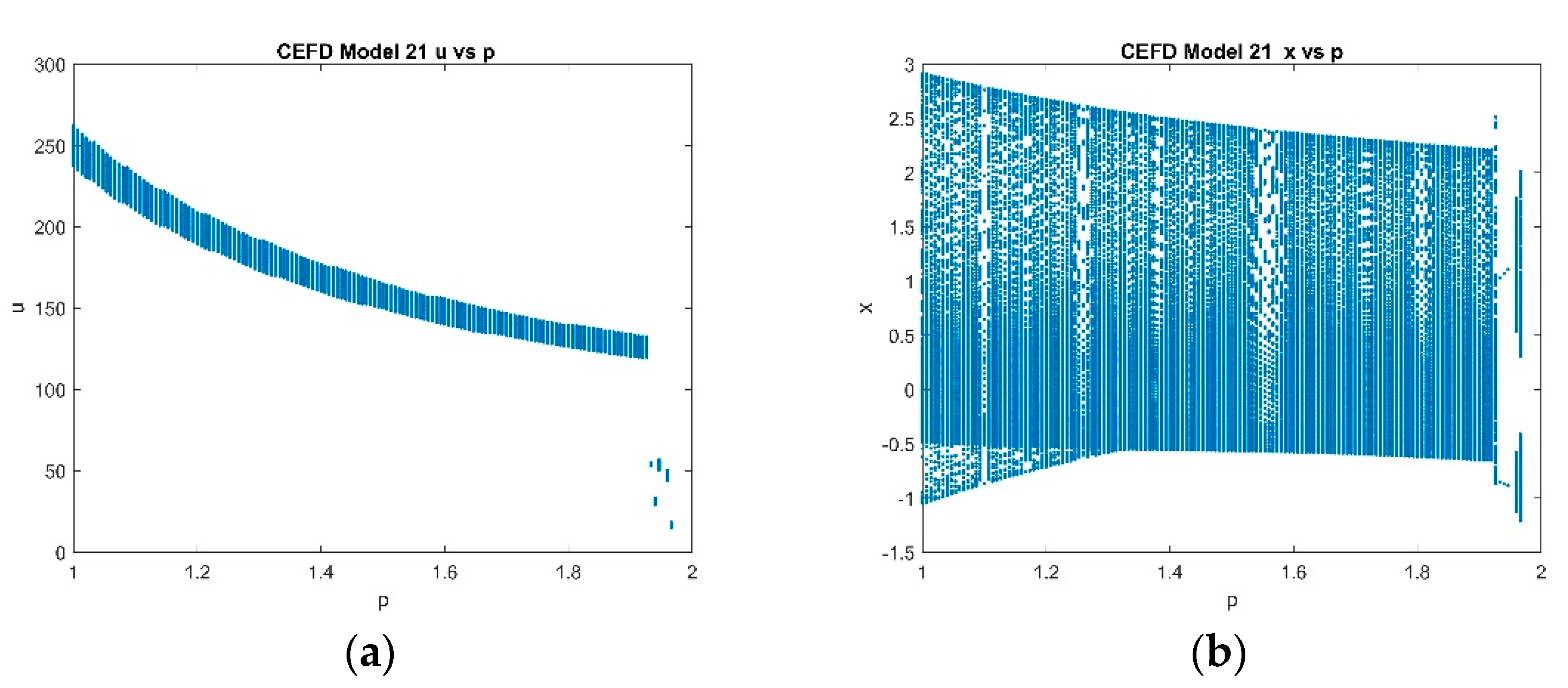
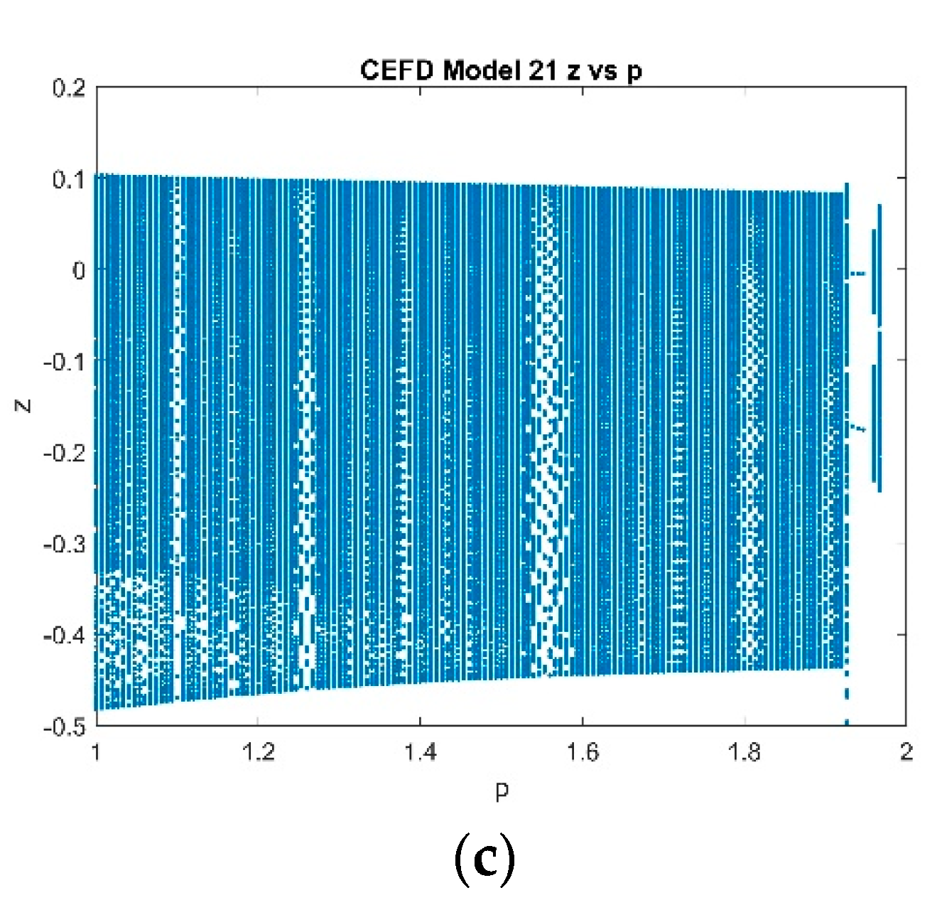
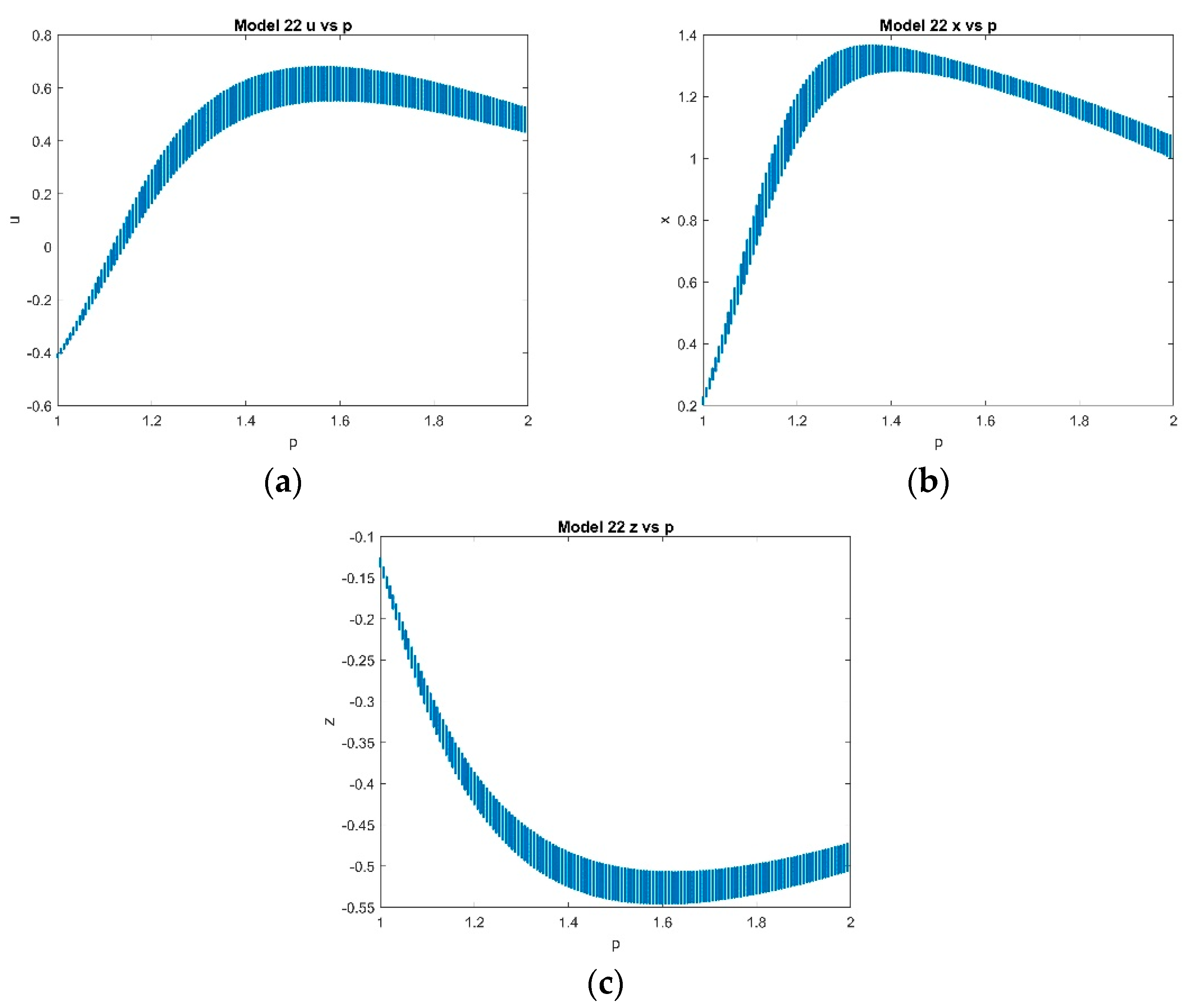
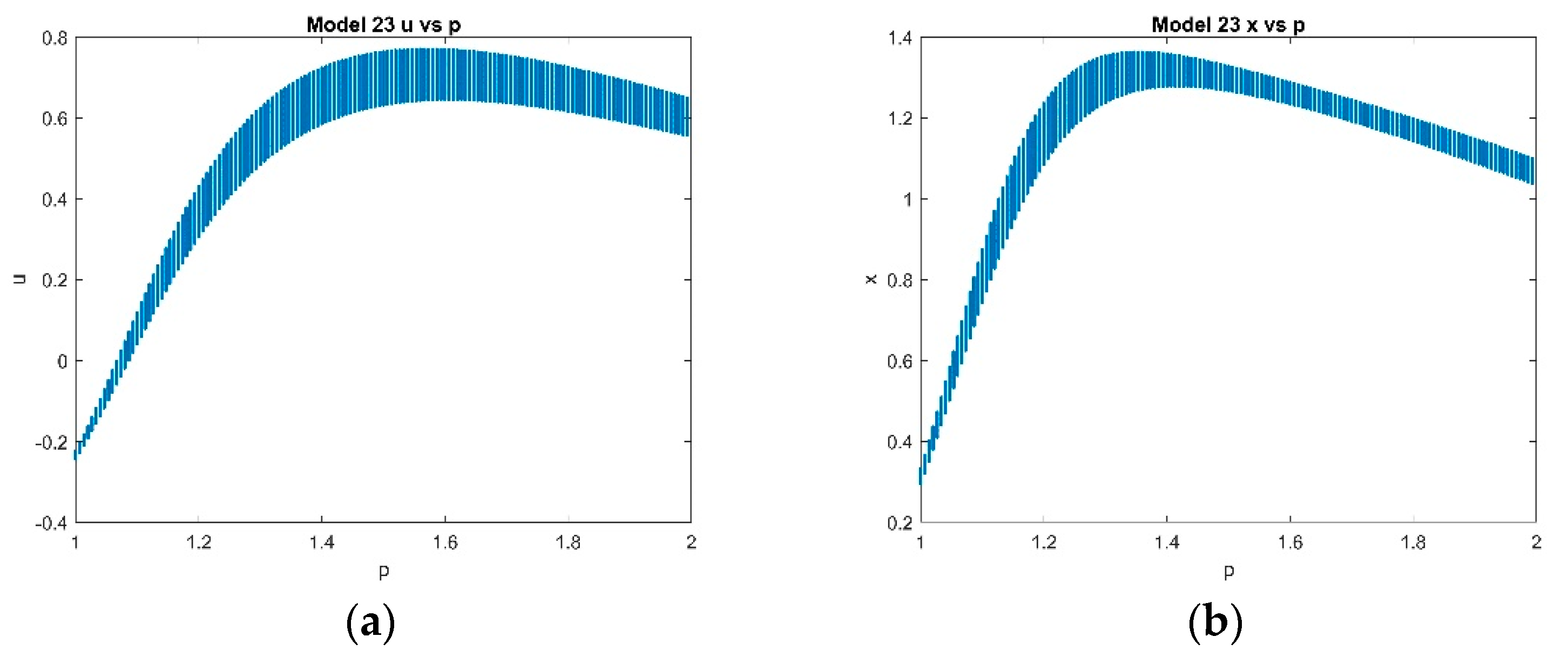
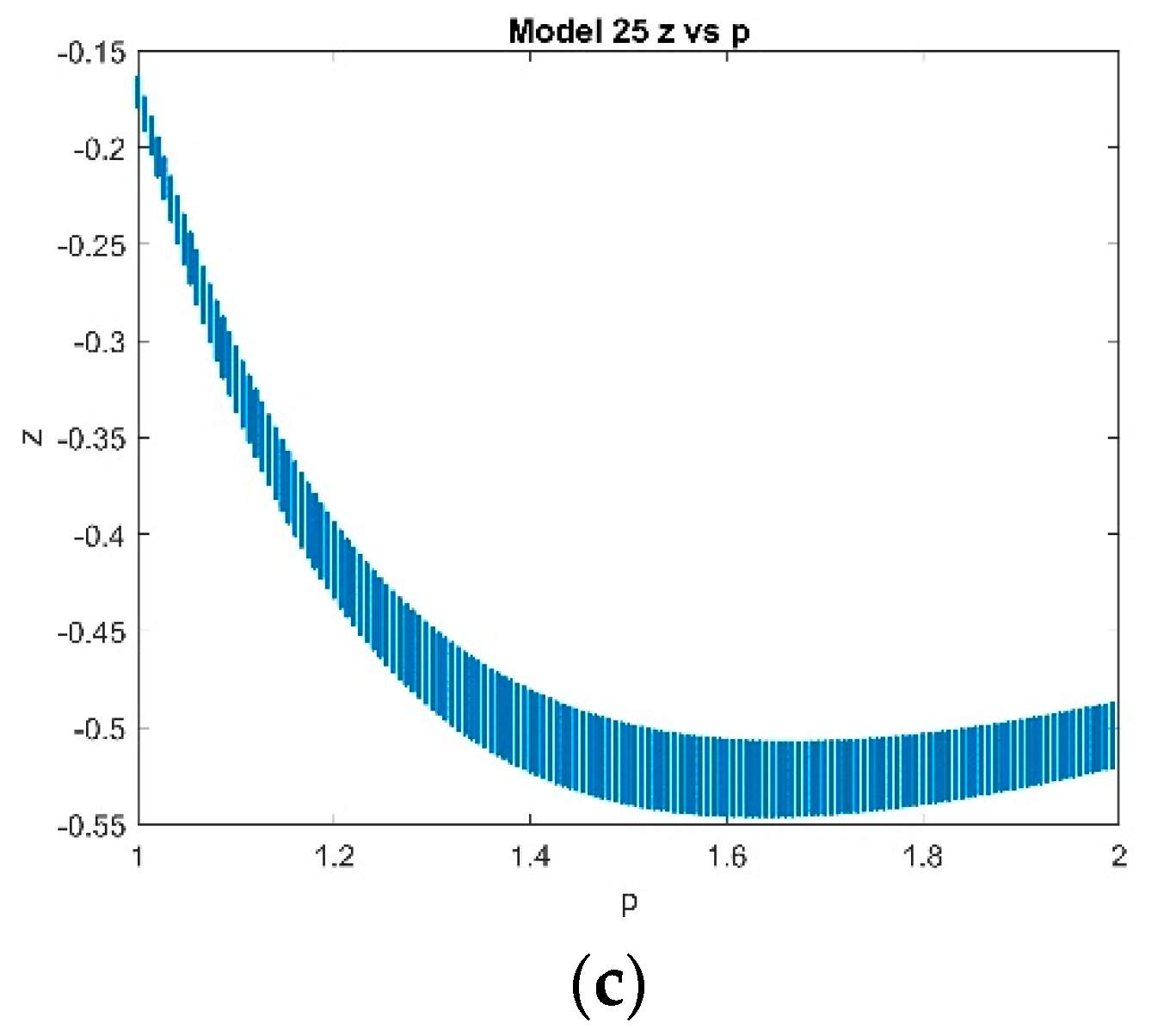
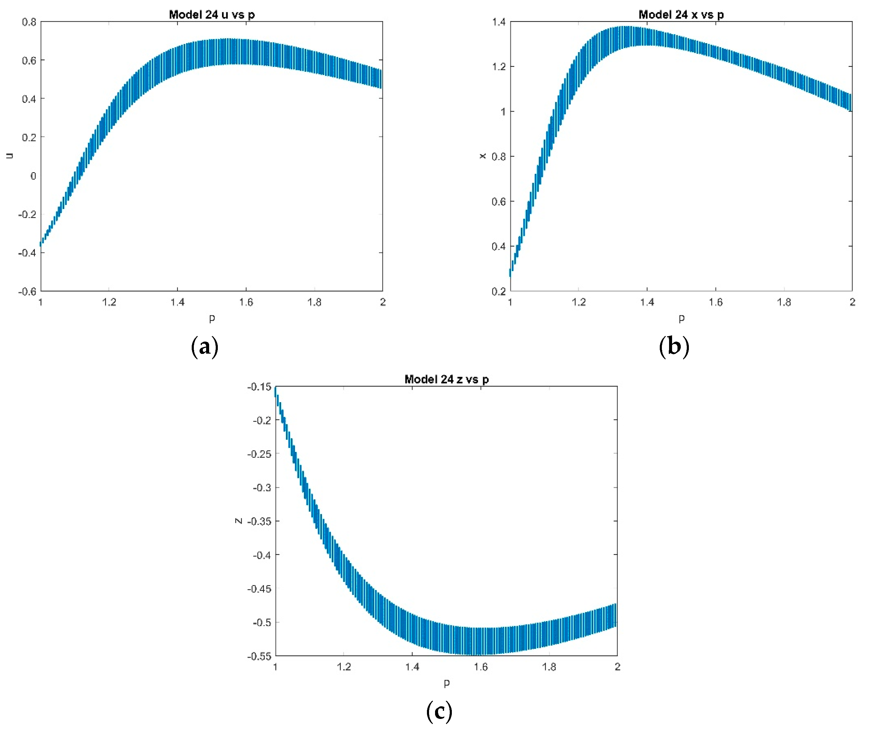
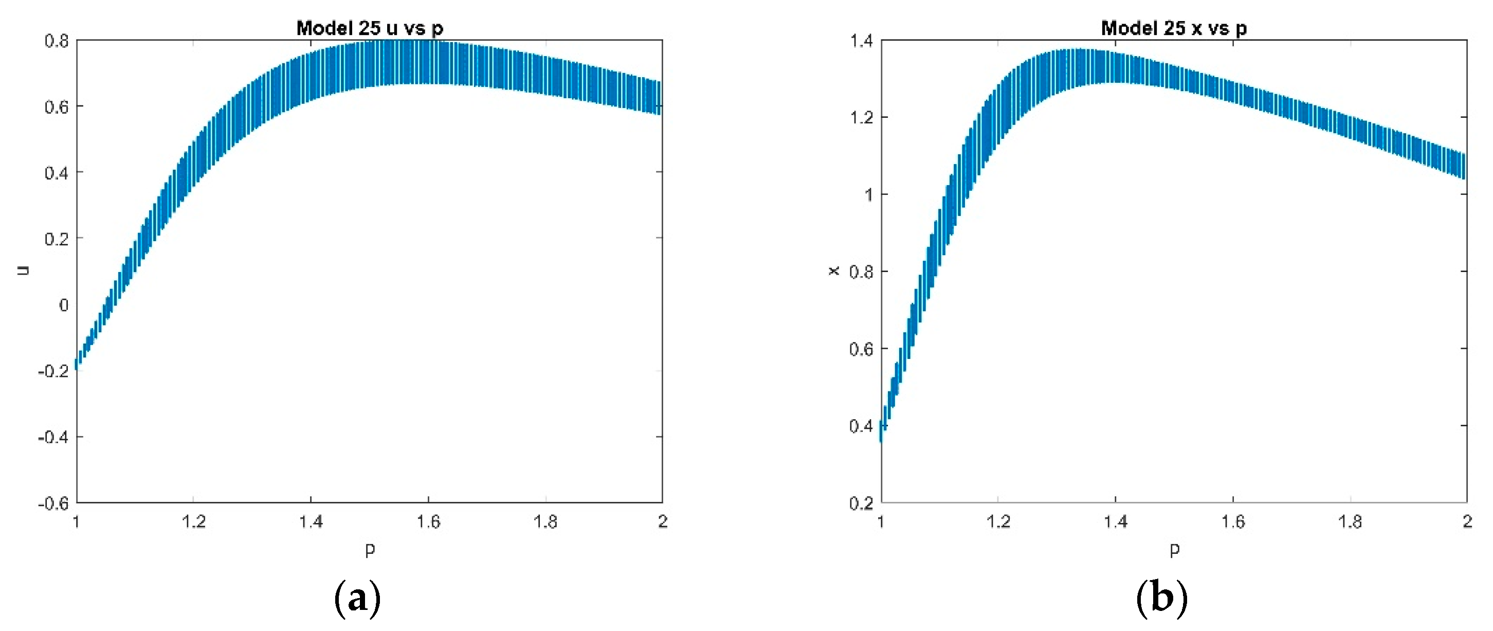
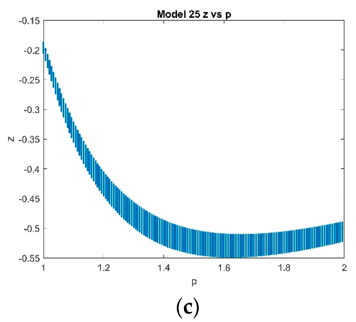
In this case, Ref. [13] concluded that system 6 is hyperchaotic with p ∈ [1, 2]. Fixing p = 1, a set of two positive Lyapunov exponents and three negative Lyapunov exponents was determined. Bifurcation tests for the ESDDFD models are performed with the same parameters for the full discrete model (2). Figure 11 shows the bifurcation diagrams for u , x and z for the CEFD model (21). Figure 12, Figure 13, Figure 14 and Figure 15 show the bifurcation diagrams for the models (22) through (25). As in Section 4.2.1, the CEFD diagrams show evidence of chaos while the other models do not.
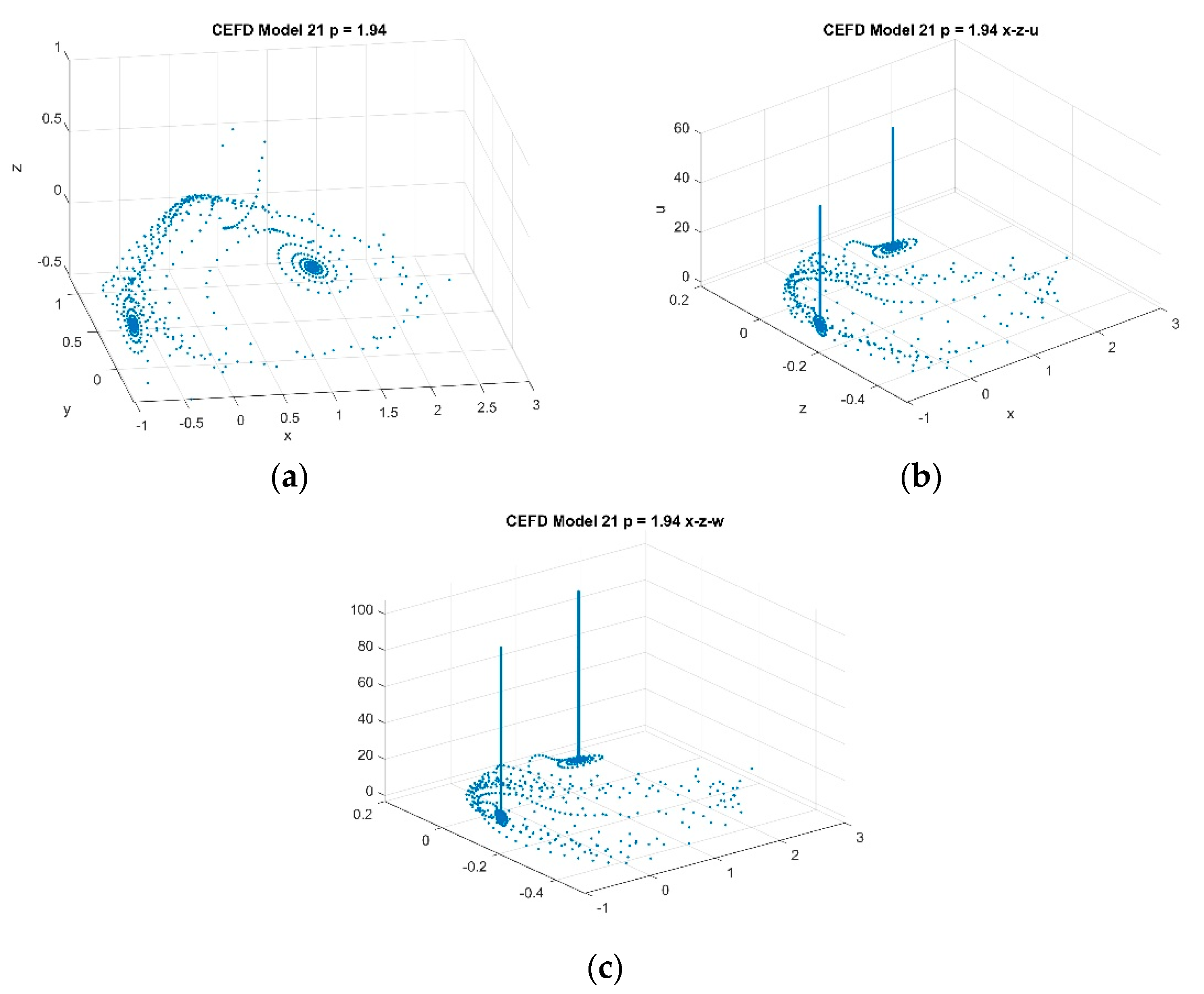
Setting p = 1.94 , phase portraits are given for models (22) through (25) in Figure 16. Figure 17 shows the phase portraits for model (21). There are clear signs of chaos in the phase portraits for model (21) and no chaos in those for the other models.

4.2.3. Varying k with Fixed p = 1 and   α 5 = 0.3 , with k ∈ [1.5, 2.5]

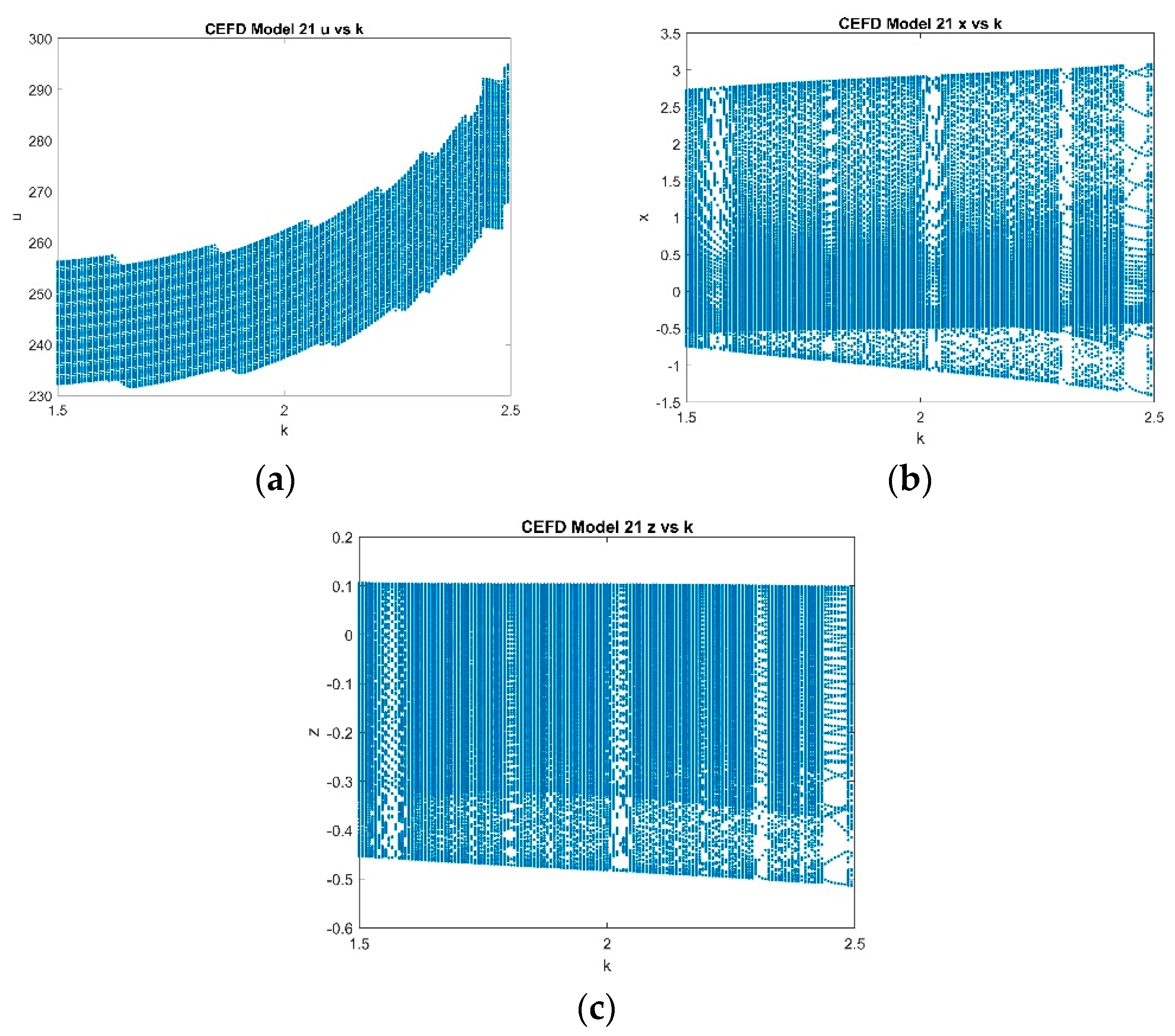
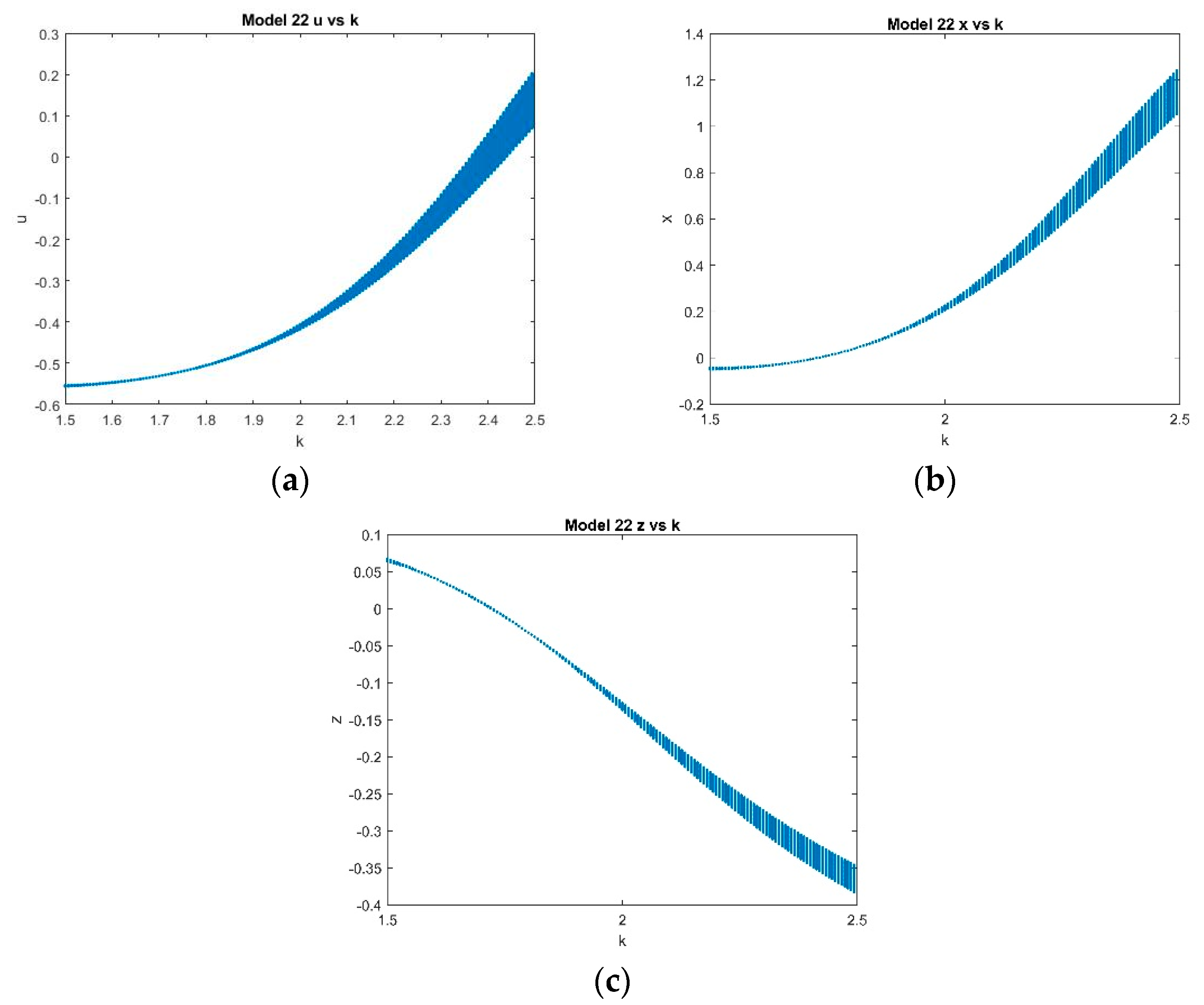
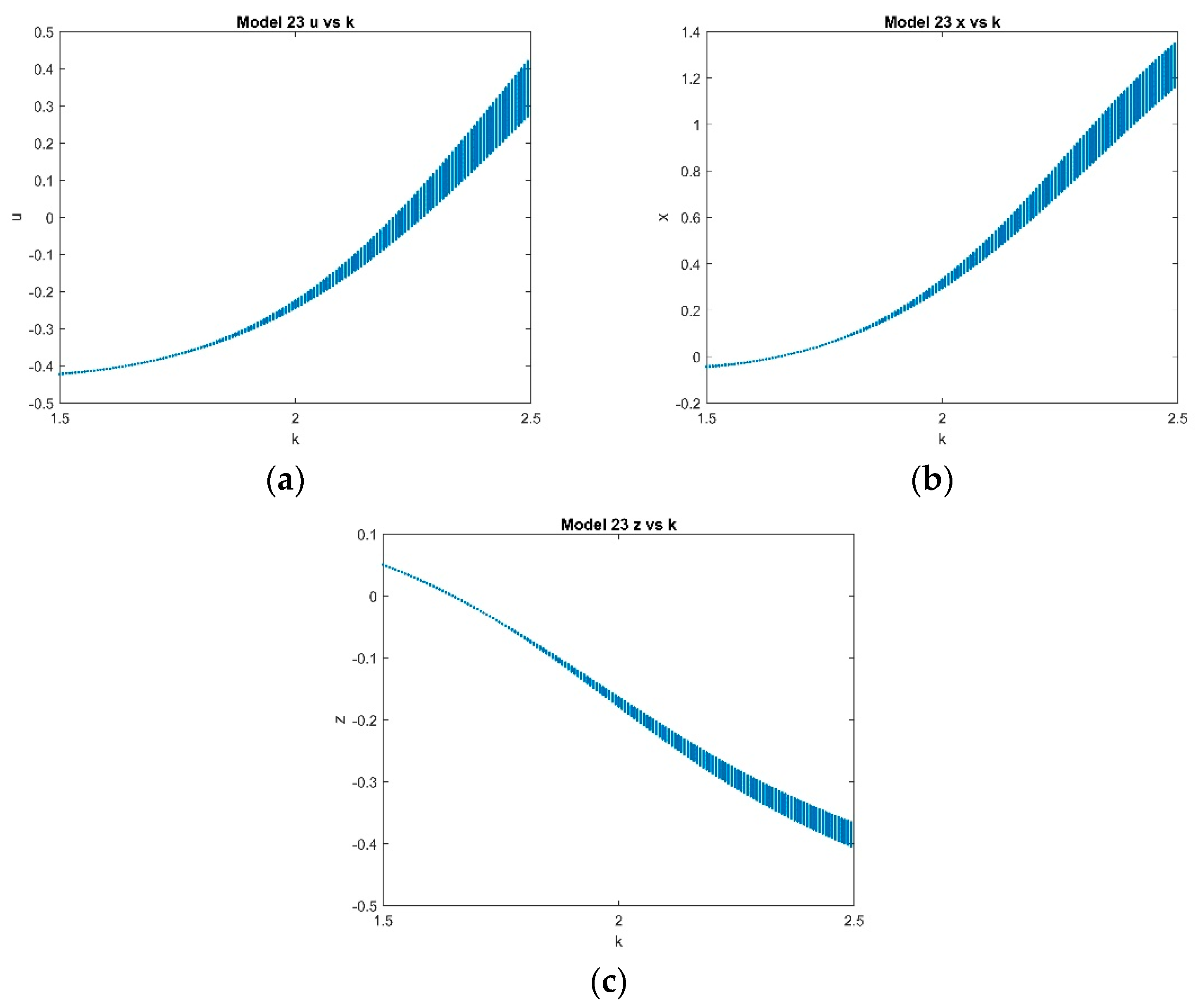
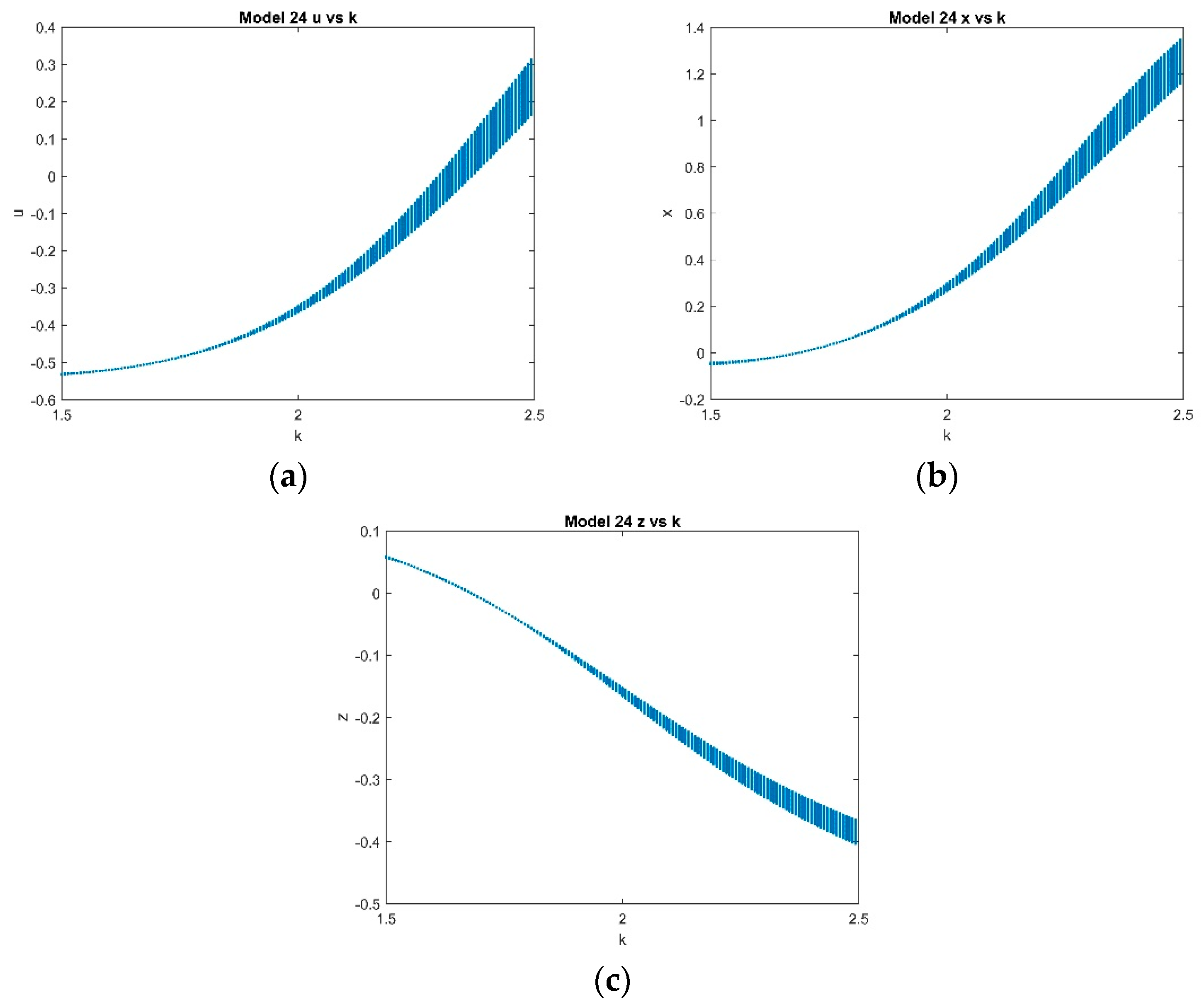
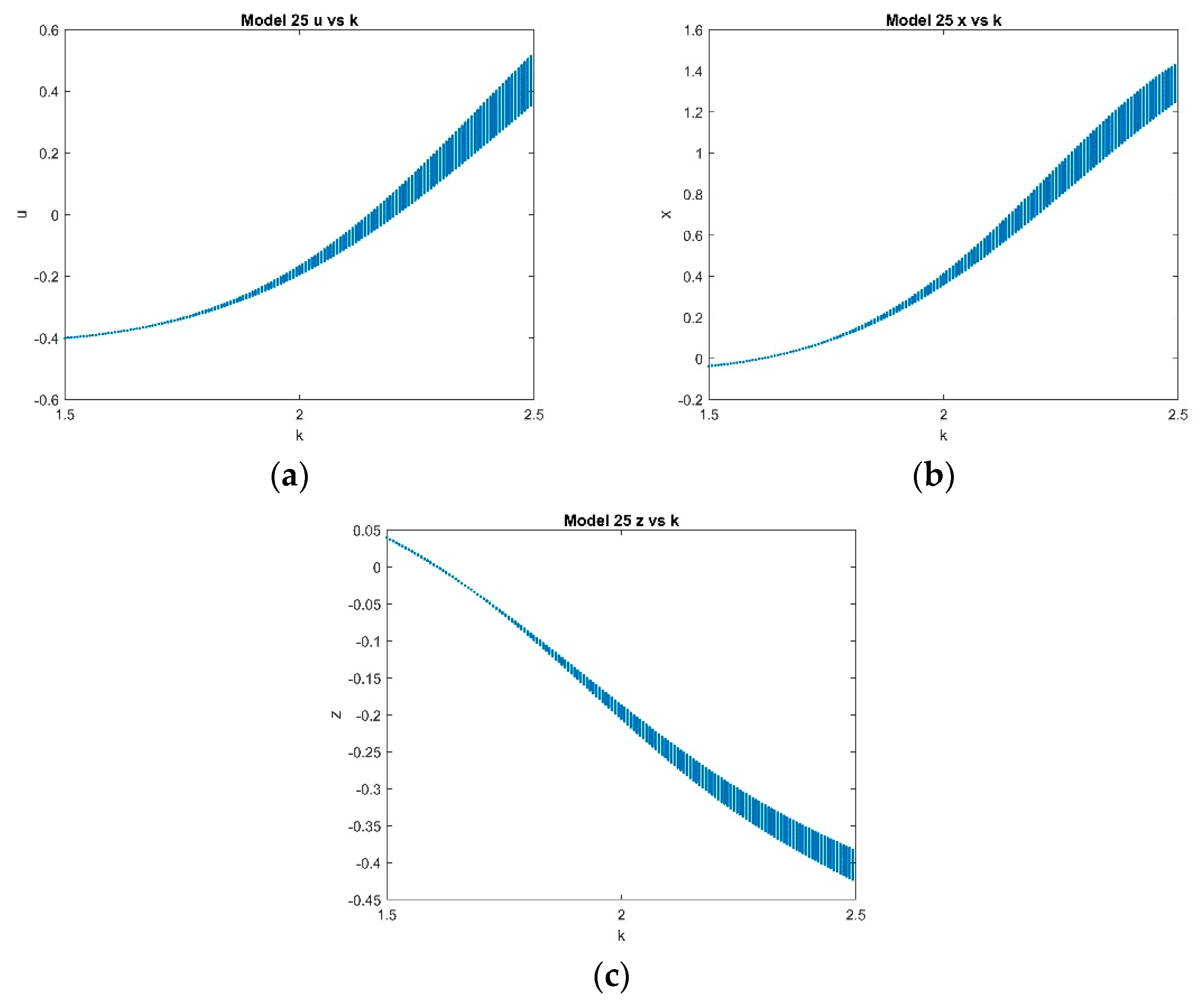
In this case, Ref. [13] concluded that system (6) is hyperchaotic with k ∈ [1.5, 2.5]. Fixing k = 1.5, a set of two positive Lyapunov exponents and three negative Lyapunov exponents were determined. Bifurcation tests for the ESDDFD models are performed with the same parameters for the full discrete model (2). Figure 18 gives the bifurcation diagrams for CEFD, model (21). Figure 19, Figure 20, Figure 21 and Figure 22 give the bifurcation diagrams for x , u and z , for models (22) through (25). Once again there is chaos evident in the CEFD diagrams but no chaos in the diagrams for the other models.
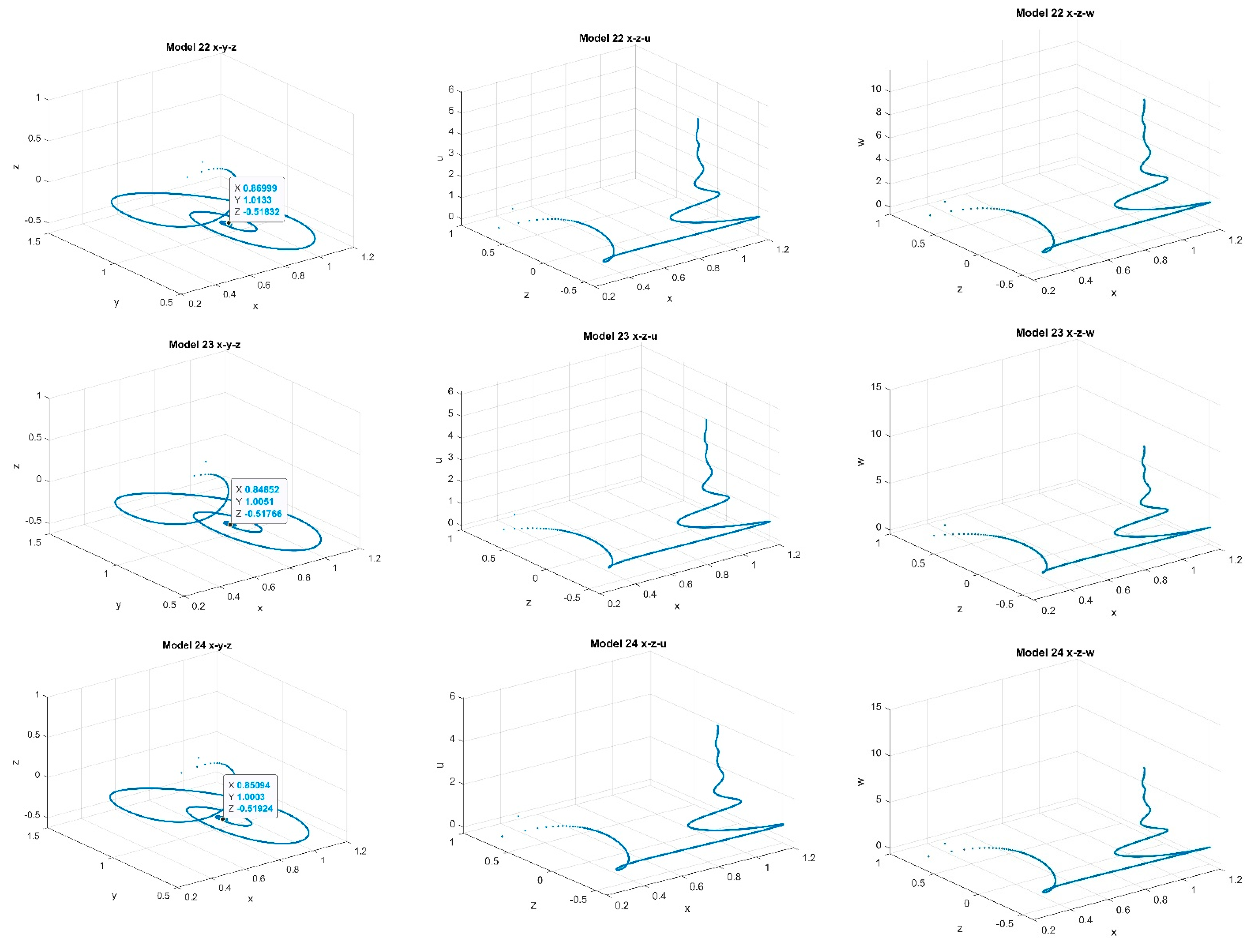
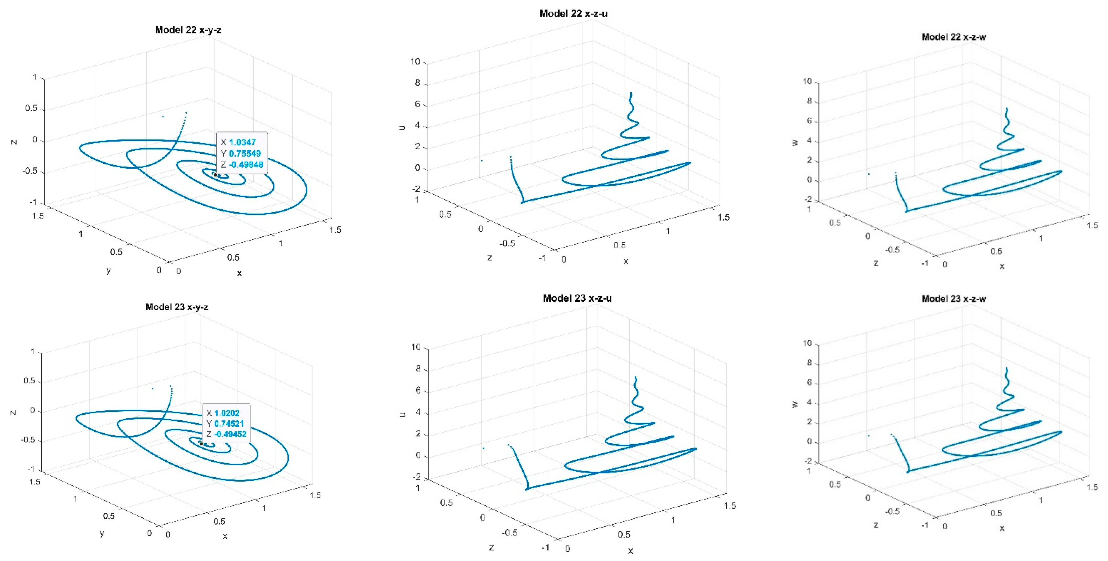
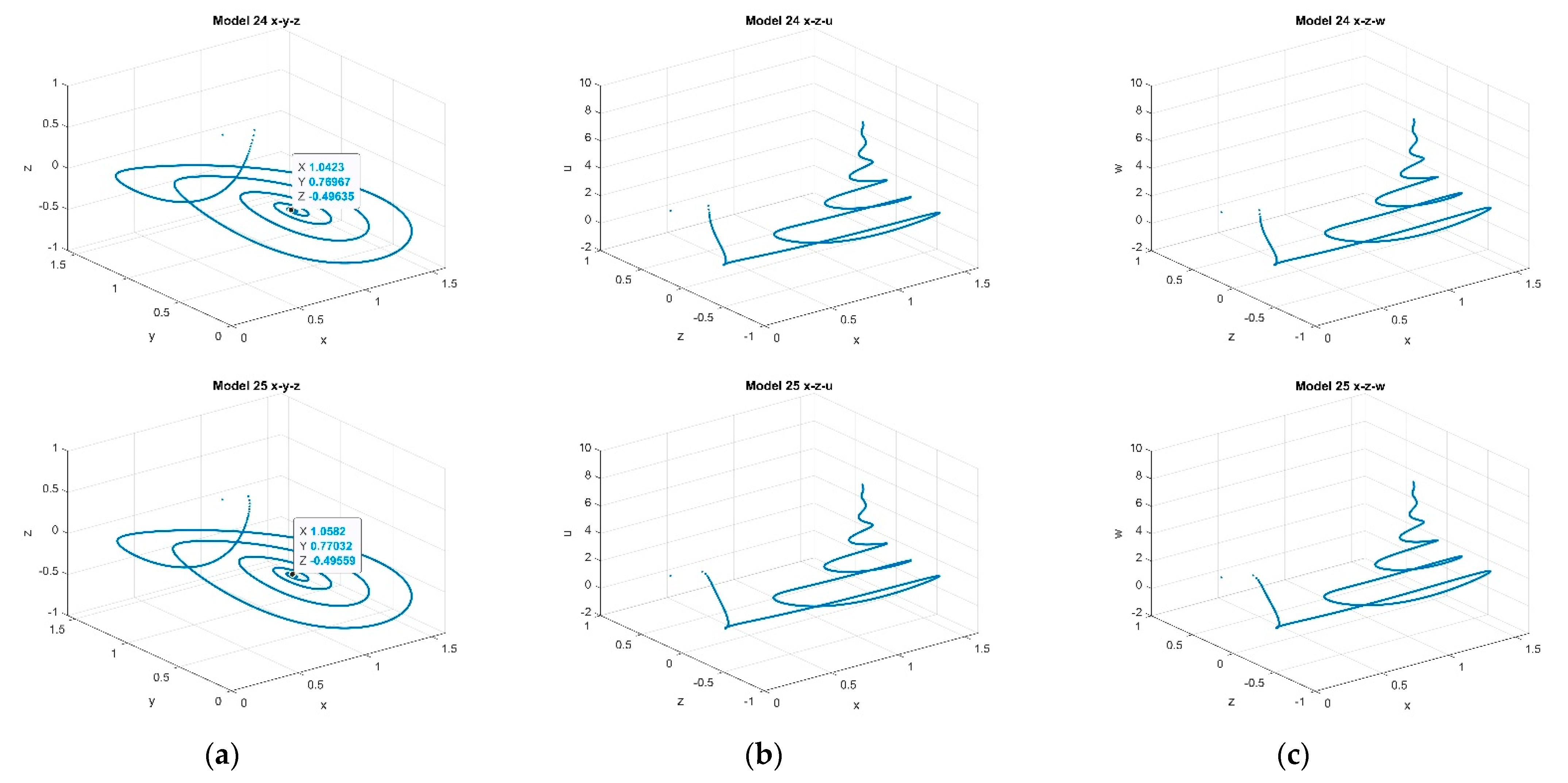
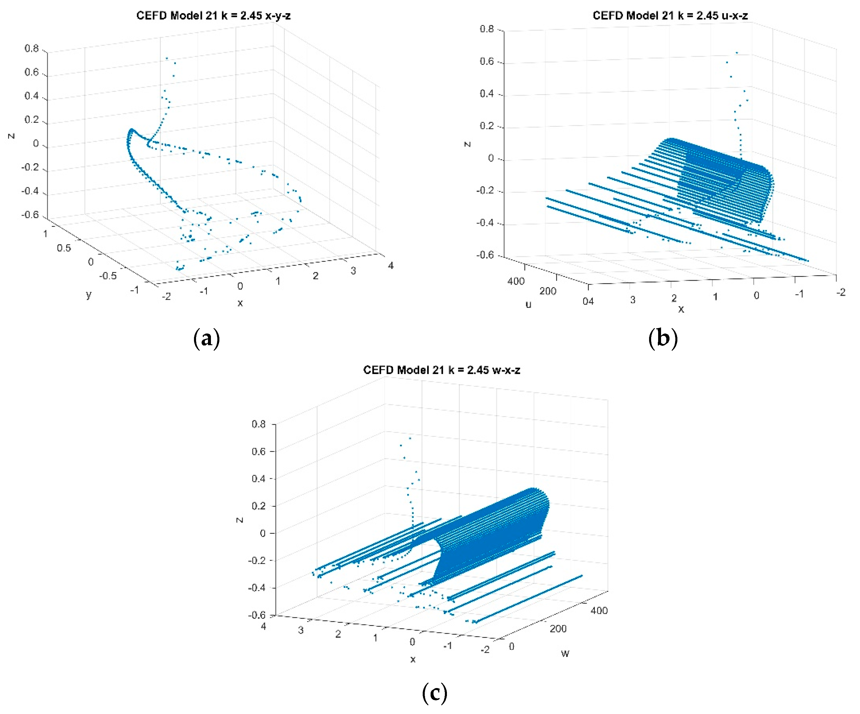
Setting k = 2.45 , phase portraits are given for models (22) through (25) in Figure 23. The phase portraits for CEFD, model (21), are given in Figure 24. Again, while the phase portraits for CEFD show chaos, it is lacking in the phase portraits for models (22) through (25).

4.2.4. With Fixed k = 2, p = 1 and α 5 = 0.24

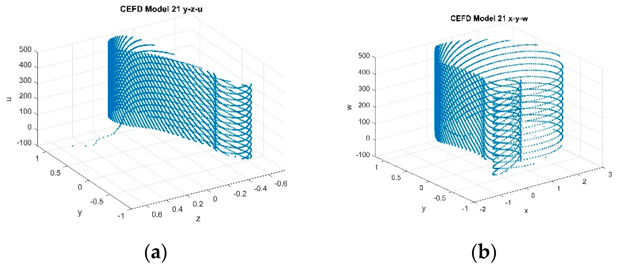
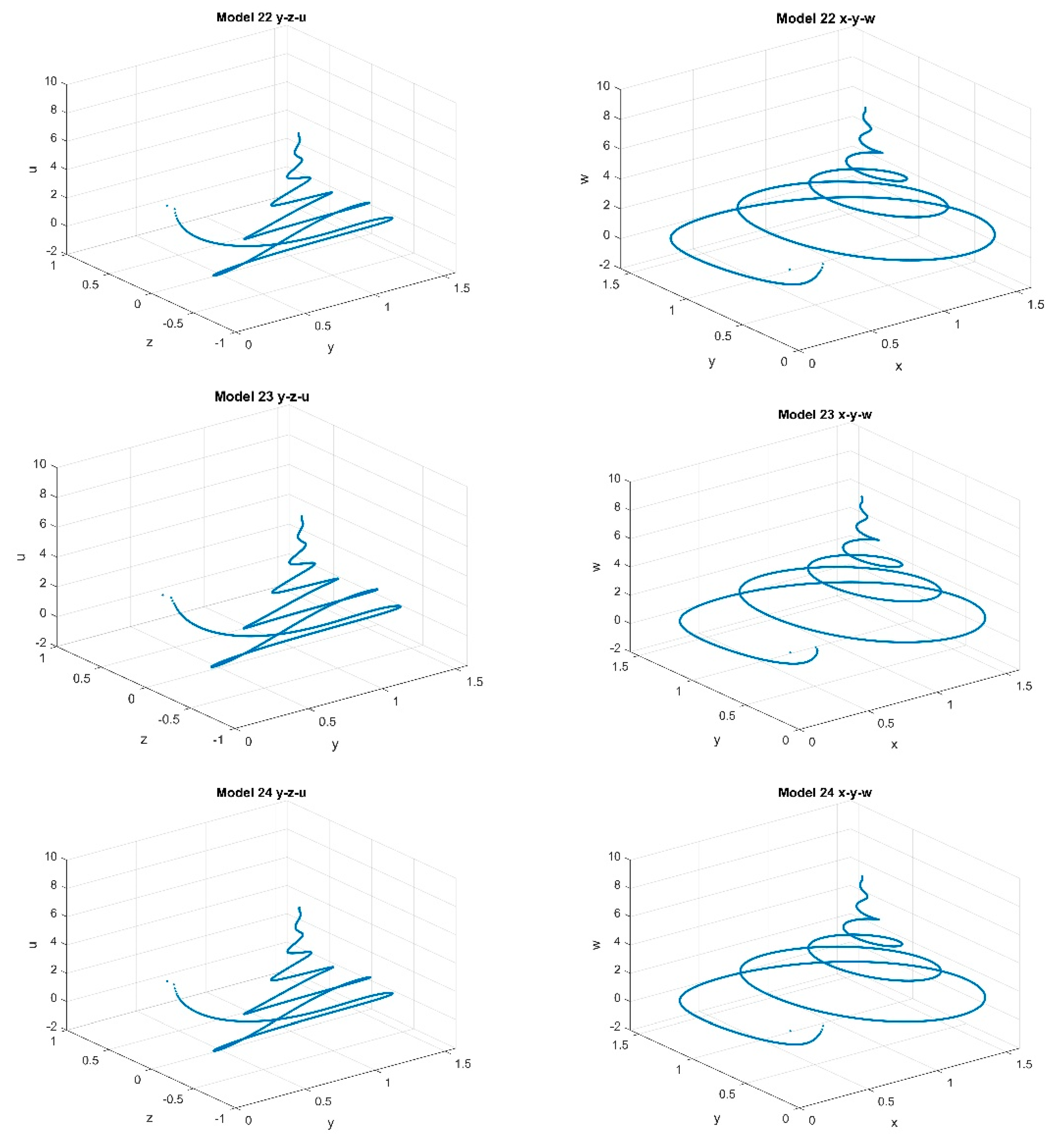
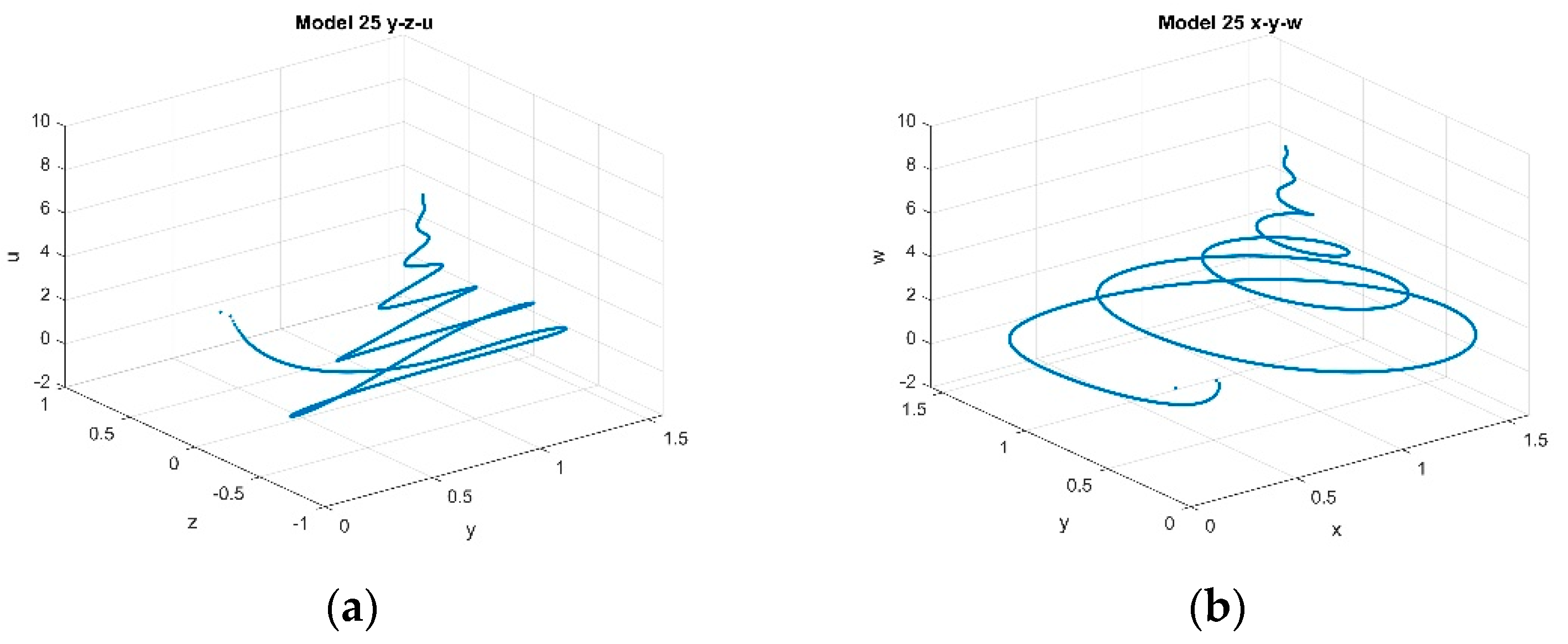
In this case, Ref. [13] concluded that system (6) has a hyperchaotic attractor in the y z u and x y w planes. Two phase portraits for model (21) are given in Figure 25 while the corresponding phase portraits for models (22) through (25) are given in Figure 26. While the results for model (21) show chaos, the results for models (22) through (25) do not.

5. Discussion

A discrete model using the conformable Euler finite difference (CEFD) model, (6), was constructed in [13] and used to detect hyperchaotic behavior of the system (1). In this paper, a discrete model (2) has been constructed for the system (1), and the parameters from [13] were used to study hyperchaos using bifurcation techniques. The discrete model (2) is constructed using the exact spectral derivative discretization finite difference (ESDDFD) method, a universal extension of the nonstandard finite difference method to fractional derivatives, which is designed to eliminate contrived chaos. Various cases are considered in parallel to those considered in [13] as well as for sub-systems relevant to the construction of the discrete model (2). While the proposed ESDDFD models produce similar results to each other, those results are significantly different from those obtained in [13] and exhibit no hyperchaotic behavior.
In view of the results obtained, it is reasonable to question the validity of the conclusions of hyperchaotic behavior previously reported for related models, which the authors intend to pursue in the future. While the conformable derivative is a local derivative and has neither memory nor nonlocality, it is a multiple of the Caputo FD [83], and therefore related to those with these properties. It will, therefore, be interesting to explore what, if any, properties of the conformable system are inherited by the Caputo and Riemann–Liouville FDs through these relationships. Further, as suggested in [13], studies incorporating real economic data with parameter estimation for the financial system with market confidence and ethics for all these derivatives are also necessary. Finally, as can be easily seen from Theorem 4.1 of [50], the discretization methods presented here for CFD systems are easy to implement and are equally applicable to all Caputo type derivatives, and hence, to Riemann–Liouville derivatives through their relationship; hence, they have potential to impact a wide range of fractional derivative applications.

Author Contributions

Conceptualization, D.P.C.-M. and G.A.G.; methodology, D.P.C.-M.; software, G.A.G.; validation, G.A.G.; formal analysis, D.P.C.-M.; writing—original draft preparation, D.P.C.-M.; writing—review and editing, D.P.C.-M. and G.A.G.; visualization, G.A.G. All authors have read and agreed to the published version of the manuscript.

Funding

This research received no external funding.

Conflicts of Interest

The authors declare no conflict of interest.

References

  1. Zhang, L.; Sun, K.; He, S.; Wang, H.; Xu, Y. Solution and dynamics of a fractional-order 5-D hyperchaotic system with four wings. Eur. Phys. J. Plus 2017, 132, 31. [Google Scholar] [CrossRef]
  2. Wang, S.; Wu, R. Dynamic analysis of a 5D fractional-order hyperchaotic system. Int. J. Control Autom. Syst. 2017, 15, 1003–1010. [Google Scholar] [CrossRef]
  3. Liu, Y.; Li, J.; Wei, Z.; Moroz, I. Bifurcation analysis and integrability in the segmented disc dynamo with mechanical friction. Adv. Differ. Equ. 2018, 2018, 210. [Google Scholar] [CrossRef] [Green Version]
  4. Wei, Z.; Moroz, I.; Sprott, J.C.; Akgul, A.; Zhang, W. Hidden hyperchaos and electronic circuit application in a 5D self-exciting homopolar disc dynamo. Chaos Interdiscip. J. Nonlinear Sci. 2017, 27, 033101. [Google Scholar] [CrossRef] [PubMed] [Green Version]
  5. Wei, Z.; Rajagopal, K.; Zhang, W.; Kingni, S.T.; Akgül, A. Synchronisation, electronic circuit implementation, and fractional-order analysis of 5D ordinary differential equations with hidden hyperchaotic attractors. Pramana 2018, 90, 50. [Google Scholar] [CrossRef]
  6. Li, C.; Chen, G. Chaos and hyperchaos in the fractional-order Rössler equations. Phys. A Stat. Mech. Appl. 2004, 341, 55–61. [Google Scholar] [CrossRef]
  7. Wang, Y.; He, S.; Wang, H.; Sun, K. Bifurcations and Synchronization of the Fractional-Order Simplified Lorenz Hyperchaotic System. J. Appl. Anal. Comput. 2015, 5, 210–219. [Google Scholar] [CrossRef]
  8. Rajagopal, K.; Karthikeyan, A.; Duraisamy, P. Hyperchaotic Chameleon: Fractional Order FPGA Implementation. Complexity 2017, 2017, 8979408. [Google Scholar] [CrossRef] [Green Version]
  9. El-Sayed, A.M.A.; Nour, H.M.; Elsaid, A.; Matouk, A.E.; Elsonbaty, A. Dynamical behaviors, circuit realization, chaos control, and synchronization of a new fractional-order hyperchaotic system. Appl. Math. Model. 2016, 40, 3516–3534. [Google Scholar] [CrossRef]
  10. El-Sayed, A.; Elsonbaty, A.; Elsadany, A.; Matouk, A. Dynamical Analysis and Circuit Simulation of a New Fractional-Order Hyperchaotic System and Its Discretization. Int. J. Bifurc. Chaos 2016, 26, 1650222. [Google Scholar] [CrossRef]
  11. Mou, J.; Sun, K.; Wang, H.; Ruan, J. Characteristic Analysis of Fractional-Order 4D Hyperchaotic Memristive Circuit. Math. Probl. Eng. 2017, 2017, 2313768. [Google Scholar] [CrossRef] [Green Version]
  12. Huang, X.; Zhao, Z.; Wang, Z.; Li, Y. Chaos and hyperchaos in fractional-order cellular neural networks. Neurocomputing 2012, 94, 13–21. [Google Scholar] [CrossRef]
  13. Xin, B.; Peng, W.; Kwon, Y.; Liu, Y. Modeling, discretization, and hyperchaos detection of conformable derivative approach to a financial system with market confidence and ethics risk. Adv. Differ. Equ. 2019, 2019, 138. [Google Scholar] [CrossRef] [Green Version]
  14. Huang, D.; Li, H. Theory and Method of the Nonlinear Economics; Sichuan University Press: Chengdu, China, 1993. [Google Scholar]
  15. Chen, W.-C. Nonlinear dynamics and chaos in a fractional-order financial system. Chaos Solitons Fractals 2008, 36, 1305–1314. [Google Scholar] [CrossRef]
  16. Wang, Z.; Huang, X.; Shen, H. Control of an uncertain fractional order economic system via adaptive sliding mode. Neurocomputing 2012, 83, 83–88. [Google Scholar] [CrossRef]
  17. Mircea, G.; Neamţu, M.; Bundău, O.; Opriş, D. Uncertain and Stochastic Financial Models with Multiple Delays. Int. J. Bifurc. Chaos 2012, 22, 1250131. [Google Scholar] [CrossRef]
  18. Xin, B.; Chen, T.; Ma, J. Neimark–Sacker Bifurcation in a Discrete-Time Financial System. Discret. Dyn. Nat. Soc. 2010, 2010, 405639. [Google Scholar] [CrossRef]
  19. Yu, H.; Cai, G.; Li, Y. Dynamic analysis and control of a new hyperchaotic finance system. Nonlinear Dyn. 2011, 67, 2171–2182. [Google Scholar] [CrossRef]
  20. Xin, B.; Li, Y. 0-1 Test for Chaos in a Fractional Order Financial System with Investment Incentive. Abstr. Appl. Anal. 2013, 2013, 876298. [Google Scholar] [CrossRef]
  21. Xin, B.; Zhang, J. Finite-time stabilizing a fractional-order chaotic financial system with market confidence. Nonlinear Dyn. 2015, 79, 1399–1409. [Google Scholar] [CrossRef]
  22. Pérez, J.E.S.; Gómez-Aguilar, J.F.; Baleanu, D.; Tchier, F. Chaotic Attractors with Fractional Conformable Derivatives in the Liouville–Caputo Sense and Its Dynamical Behaviors. Entropy 2018, 20, 384. [Google Scholar] [CrossRef] [Green Version]
  23. Eslami, M.; Rezazadeh, H. The first integral method for Wu–Zhang system with conformable time-fractional derivative. Calcolo 2016, 53, 475–485. [Google Scholar] [CrossRef]
  24. Ilie, M.; Biazar, J.; Ayati, Z. The first integral method for solving some conformable fractional differential equations. Opt. Quantum Electron. 2018, 50, 55. [Google Scholar] [CrossRef]
  25. Hosseini, K.; Bekir, A.; Ansari, R. New exact solutions of the conformable time-fractional Cahn–Allen and Cahn–Hilliard equations using the modified Kudryashov method. Optik 2017, 132, 203–209. [Google Scholar] [CrossRef]
  26. Ünal, E.; Gökdoğan, A. Solution of conformable fractional ordinary differential equations via differential transform method. Optik 2017, 128, 264–273. [Google Scholar] [CrossRef] [Green Version]
  27. Kumar, D.; Seadawy, A.R.; Joardar, A.K. Modified Kudryashov method via new exact solutions for some conformable fractional differential equations arising in mathematical biology. Chin. J. Phys. 2018, 56, 75–85. [Google Scholar] [CrossRef]
  28. Srivastava, H.; Gunerhan, H. Analytical and approximate solutions of fractional-order susceptible-infected-recovered epidemic model of childhood disease. Math. Methods Appl. Sci. 2019, 42, 935–941. [Google Scholar] [CrossRef]
  29. Kaplan, M. Applications of two reliable methods for solving a nonlinear conformable time-fractional equation. Opt. Quantum Electron. 2017, 49, 312. [Google Scholar] [CrossRef]
  30. Yavuz, M.; Özdemir, N. A different approach to the European option pricing model with new fractional operator. Math. Model. Nat. Phenom. 2018, 13, 12. [Google Scholar] [CrossRef] [Green Version]
  31. Kartal, S.; Gurcan, F. Discretization of conformable fractional differential equations by a piecewise constant approximation. Int. J. Comput. Math. 2018, 96, 1849–1860. [Google Scholar] [CrossRef]
  32. Iyiola, O.; Tasbozan, O.; Kurt, A.; Cenesiz, Y. On the analytical solutions of the system of conformable time-fractional Robertson equations with 1-D diffusion. Chaos Solitons Fractals 2017, 94, 1–7. [Google Scholar] [CrossRef]
  33. Ruan, J.; Sun, K.; Mou, J.; He, S.; Zhang, L. Fractional-order simplest memristor-based chaotic circuit with new derivative. Eur. Phys. J. Plus 2018, 133, 3. [Google Scholar] [CrossRef]
  34. He, S.; Sun, K.; Mei, X.; Yan, B.; Xu, S. Numerical analysis of a fractional-order chaotic system based on conformable fractional-order derivative. Eur. Phys. J. Plus 2017, 132, 36. [Google Scholar] [CrossRef]
  35. Yokus, A. Comparison of Caputo and conformable derivatives for time-fractional Korteweg-de Vries equation via the finite differencemethod. Int. J. Mod. Phys. B 2018, 32, 1850365. [Google Scholar] [CrossRef]
  36. Rezazadeh, H.; Ziabarya, B. Sub-equation method for the conformable fractional generalized Kuramoto–Sivashinsky equation. Comput. Res. Prog. App. Sci. Eng. 2016, 2, 106–109. [Google Scholar]
  37. Zhong, W.; Wang, L. Basic theory of initial value problems of conformable fractional differential equations. Adv. Differ. Equ. 2018, 2018, 321. [Google Scholar] [CrossRef]
  38. Tayyan, B.A.; Sakka, A.H. Lie symmetry analysis of some conformable fractional partial differential equations. Arab. J. Math. 2018, 9, 201–212. [Google Scholar] [CrossRef] [Green Version]
  39. Yaslan, H. Numerical solution of the conformable space-time fractional wave equation. Chin. J. Phys. 2018, 56, 2916–2925. [Google Scholar] [CrossRef]
  40. Kurt, A.; Çenesiz, Y.; Tasbozan, O. On the Solution of Burgers’ Equation with the New Fractional Derivative. Open Phys. 2015, 13, 355–360. [Google Scholar] [CrossRef] [Green Version]
  41. Khalil, R.; Abu-Shaab, H. Solution of some conformable fractional differential equations. Int. J. Pure Appl. Math. 2015, 103, 667–673. [Google Scholar] [CrossRef] [Green Version]
  42. Unal, E.; Gokdogan, A.; Celik, E. Solutions of sequential conformable fractional differential equations around an ordinary point and conformable fractional Hermite differential equation. arXiv 2015, arXiv:1503.05407. [Google Scholar]
  43. Liu, S.; Wang, H.; Li, X.; Li, H. The extremal iteration solution to a coupled system of nonlinear conformable fractional differential equations. J. Nonlinear Sci. Appl. 2017, 10, 5082–5089. [Google Scholar] [CrossRef] [Green Version]
  44. Çenesiz, Y.; Kurt, A. The solutions of time and space conformable fractional heat equations with conformable Fourier transform. Acta Univ. Sapientiae Math. 2015, 7, 130–140. [Google Scholar] [CrossRef] [Green Version]
  45. El-Sayed, A.; Salman, S. On a discretization process of fractional-order Riccati differential equation. J. Fract. Calc. Appl. 2013, 4, 251–259. [Google Scholar]
  46. Agarwal, R.; El-Sayed, A.; Salman, S. Fractional-order Chua’s system: Discretization, bifurcation and chaos. Adv. Differ. Equ. 2013, 1, 320. [Google Scholar] [CrossRef]
  47. Mohammadnezhad, V.; Eslami, M.; Rezazadeh, H. Stability analysis of linear conformable fractional differential equations system with time delays. Bol. Soc. Parana. Mat. 2020, 38, 159–171. [Google Scholar] [CrossRef]
  48. Micken, R.E. Nonstandard Finite Difference Schemes: Methodology and Applications; World Scientific Publishing Company: Singapore, 2020. [Google Scholar]
  49. Garba, S.; Gumel, A.; Lubuma, J. Dynamically-consistent non-standard finite difference method for an epidemic model. Math. Comput. Model. 2011, 53, 131–150. [Google Scholar] [CrossRef]
  50. Clemence-Mkhope, D.P.; Clemence-Mkhope, B.G.B. The Limited Validity of the Conformable Euler Finite Difference Method and an Alternate Definition of the Conformable Fractional Derivative to Justify Modification of the Method. Math. Comput. Appl. 2021, 26, 66. [Google Scholar] [CrossRef]
  51. Clemence-Mkhope, D.P. The Exact Spectral Derivative Discretization Finite Difference (ESDDFD) Method for Wave Models. arXiv 2021, arXiv:2106.07609. [Google Scholar]
  52. Clemence-Mkhope, D.P. Spectral Non-integer Derivative Representations and the Exact Spectral Derivative Discretization Finite Difference Method for the Fokker–Planck Equation. arXiv 2021, arXiv:2106.02586. [Google Scholar]
  53. Zheng, R.; Jiang, X. Spectral methods for the time-fractional Navier-Stokes equation. Appl. Math. Lett. 2019, 91, 194–200. [Google Scholar] [CrossRef]
  54. Xu, H.; Jiang, X. Creep constitutive models for viscoelastic materials based on fractional derivatives. Comput. Math. Appl. 2017, 73, 1377–1384. [Google Scholar] [CrossRef]
  55. Fan, W.; Qi, H. An efficient finite element method for the two-dimensional nonlinear time–space fractional Schrödinger equation on an irregular convex domain. Appl. Math. Lett. 2018, 86, 103–110. [Google Scholar] [CrossRef]
  56. Yang, X.; Qi, H.; Jiang, X. Numerical analysis for electroosmotic flow of fractional Maxwell fluids. Appl. Math. Lett. 2018, 78, 1–8. [Google Scholar] [CrossRef]
  57. Gao, X.; Chen, D.; Yan, D.; Xu, B.; Wang, X. Dynamic evolution characteristics of a fractional order hydropower station system. Mod. Phys. Lett. B 2018, 32, 1750363. [Google Scholar] [CrossRef]
  58. Wang, F.; Chen, D.; Zhang, X.; Wu, Y. Finite-time stability of a class of nonlinear fractional-order system with the discrete time delay. Int. J. Syst. Sci. 2017, 48, 984–993. [Google Scholar] [CrossRef]
  59. Wu, G.-C.; Baleanu, D.; Huang, L.-L. Novel Mittag–Leffler stability of linear fractional delay difference equations with impulse. Appl. Math. Lett. 2018, 82, 71–78. [Google Scholar] [CrossRef]
  60. Wu, G.-C.; Baleanu, D.; Luo, W.-H. Analysis of fractional non-linear diffusion behaviors based on Adomian polynomials. Therm. Sci. 2017, 21, 813–817. [Google Scholar] [CrossRef]
  61. Khalil, R.; Al Horani, M.; Yousef, A.; Sababheh, M. A new definition of fractional derivative. J. Comput. Appl. Math. 2014, 264, 65–70. [Google Scholar] [CrossRef]
  62. Abdeljawad, T. On conformable fractional calculus. J. Comput. Appl. Math. 2015, 279, 57–66. [Google Scholar] [CrossRef]
  63. Abdeljawad, T.; Al-Mdallal, Q.; Jarad, F. Fractional logistic models in the frame of fractional operators generated by conformable derivatives. Chaos Solitons Fractals 2019, 119, 94–101. [Google Scholar] [CrossRef]
  64. Imbert Alberto, F. Contributions to Conformable and Non-Conformable Calculus. Ph.D. Thesis, Universidad Carlos III de Madrid, Madrid, Spain, 2019. Available online: https://www.researchgate.net/publication/342654962_Contributions_to_Conformable_and_non-Conformable_Calculus (accessed on 28 May 2021).
  65. Acan, O.; Firat, O.; Keskin, Y. Conformable variational iteration method, conformable fractional reduced differential transform method and conformable homotopy analysis method for non-linear fractional partial differential equations. Waves Random Complex Media 2018, 8, 1–19. [Google Scholar] [CrossRef]
  66. Attia, R.A.M.; Lu, D.; Khater, M.M.A. Chaos and Relativistic Energy-Momentum of the Nonlinear Time Fractional Duffing Equation. Math. Comput. Appl. 2019, 24, 10. [Google Scholar] [CrossRef] [Green Version]
  67. Bohner, M.; Hatipoğlu, V.F. Dynamic cobweb models with conformable fractional derivatives. Nonlinear Anal. Hybrid Syst. 2018, 32, 157–167. [Google Scholar] [CrossRef]
  68. Tarasov, V. No nonlocality. No fractional derivative. Commun. Nonlinear Sci. Numer. Simul. 2018, 62, 157–163. [Google Scholar] [CrossRef] [Green Version]
  69. Rosales, J.; Godínez, F.; Banda, V.; Valencia, G. Analysis of the Drude model in view of the conformable derivative. Optik 2018, 178, 1010–1015. [Google Scholar] [CrossRef]
  70. Akbulut, A.; Melike, K. Auxiliary equation method for time-fractional differential equations with conformable derivative. Comput. Math. Appl. 2018, 75, 876–882. [Google Scholar] [CrossRef]
  71. Martínez, L.; Rosales, J.; Carreño, C.; Lozano, J. Electrical circuits described by fractional conformable derivative. Int. J. Circuit Theory Appl. 2018, 46, 1091–1100. [Google Scholar] [CrossRef]
  72. Rezazadeh, H.; Khodadad, F.; Manafian, J. New structure for exact solutions of nonlinear time fractional Sharma–Tasso–Olver equation via conformable fractional derivative. Appl. Appl. Math. 2017, 12, 13–21. [Google Scholar]
  73. Korkmaz, A. Explicit exact solutions to some one-dimensional conformable time fractional equations. Waves Random Complex Media 2017, 29, 124–137. [Google Scholar] [CrossRef]
  74. He, S.; Banerjee, S.; Yan, B. Chaos and Symbol Complexity in a Conformable Fractional-Order Memcapacitor System. Complexity 2018, 2018, 4140762. [Google Scholar] [CrossRef]
  75. Xin, B.; Chen, T.; Liu, Y. Synchronization of chaotic fractional-order WINDMI systems via linear state error feedback control. Math. Probl. Eng. 2010, 2010, 859685. [Google Scholar] [CrossRef] [Green Version]
  76. Yavuz, M.; Özdemir, N. European Vanilla Option Pricing Model of Fractional Order without Singular Kernel. Fractal Fract. 2018, 2, 3. [Google Scholar] [CrossRef] [Green Version]
  77. Baskonus, H.M.; Mekkaoui, T.; Hammouch, Z.; Bulut, H. Active Control of a Chaotic Fractional Order Economic System. Entropy 2015, 17, 5771–5783. [Google Scholar] [CrossRef] [Green Version]
  78. Ma, J.; Ren, W. Complexity and Hopf Bifurcation Analysis on a Kind of Fractional-Order IS-LM Macroeconomic System. Int. J. Bifurc. Chaos 2016, 26, 1650181. [Google Scholar] [CrossRef] [Green Version]
  79. Huang, Y.; Wang, N.; Zhang, J.; Guo, F. Controlling and synchronizing a fractional-order chaotic system using stability theory of a time-varying fractional-order system. PLoS ONE 2018, 13, e0194112. [Google Scholar] [CrossRef] [PubMed] [Green Version]
  80. Xin, B.; Chen, T.; Liu, Y. Projective synchronization of chaotic fractional-order energy resources demand–supply systems via linear control. Commun. Nonlinear Sci. Numer. Simul. 2011, 16, 4479–4486. [Google Scholar] [CrossRef]
  81. Almeida, R.; Malinowska, A.B.; Monteiro, T. Fractional differential equations with a Caputo derivative with respect to a Kernel function and their applications. Math. Methods Appl. Sci. 2017, 41, 336–352. [Google Scholar] [CrossRef] [Green Version]
  82. Anderson, D.R.; Camrud, E.; Ulness, D.J. On the nature of the conformable derivative and its applications to physics. J. Fract. Calc. Appl. 2019, 10, 92–135. [Google Scholar]
  83. Mainardi, F. A Note on the Equivalence of Fractional Relaxation Equations to Differential Equations with Varying Coefficients. Mathematics 2018, 6, 8. [Google Scholar] [CrossRef] [Green Version]
Figure 1. Phase portraits (a) CEFD model (20) (b) MCEFD model (16) (c) Model 17 (d) Model 18 (e) model (19).
Mca 27 00004 g001
Figure 2. CEFD model (21) profiles of (a) x y z , (b) x u z , (c) x w z , at h = 0.002 ,   k = 2 ,   p = 1 ,   α 5 = 0.232 .
Mca 27 00004 g002
Figure 3. Phase portraits (a) x y z , (b) x u z ,   (c) x z w , at h = 0.002 ,   k = 2 ,   p = 1 ,   α 5 = 0.232 for models (22) through (25).
Mca 27 00004 g003
Figure 4. CEFD model (21); bifurcation of (a) u (b) x (c) z versus α 5 for h = 0.002 .
Mca 27 00004 g004
Figure 5. MCEFD Model (22); (a) u   vs .   α 5 , (b) x   vs .   α 5 , (c) z   vs .   α 5 , at k = 2 ,   p = 1 , α 5 [ 0.232 ,   0.328 ] .
Mca 27 00004 g005
Figure 6. ESDDFD model (23); (a) u   vs .   α 5 , (b) x   vs .   α 5 , (c) z   vs .   α 5 , at k = 2 ,   p = 1 , α 5 [ 0.232 ,   0.328 ] .
Mca 27 00004 g006
Figure 7. ESDDFD model (24); (a) u   vs .   α 5 , (b) x   vs .   α 5 , (c) z   vs .   α 5 , at k = 2 ,   p = 1 , α 5 [ 0.232 ,   0.328 ] .
Mca 27 00004 g007
Figure 8. ESDDFD model (25); (a) u   vs .   α 5 , (b) x   vs .   α 5 , (c) z   vs .   α 5 , at k = 2 ,   p = 1 , α 5 [ 0.232 ,   0.328 ] .
Mca 27 00004 g008
Figure 9. Phase portraits (a) x y z , (b) x u z , (c) x z w , at h = 0.1 ,   k = 2 ,   p = 1 ,   α 5 = 0.232 for models (22) through (25).
Mca 27 00004 g009aMca 27 00004 g009b
Figure 10. Phase portraits (a) x y z , (b) x u z , (c) x z w , at h = 1.0 ,   k = 2 ,   p = 1 ,   α 5 = 0.232 for models (22) through (25). h = 1.0 ,   α 5 = 0.232 for (23) through (25).
Mca 27 00004 g010aMca 27 00004 g010b
Figure 11. CEFD model (21); (a) u   vs .   p , (b) x   vs .   p , (c) z   vs .   p , at k = 2 ,   α 5 = 0.3 ,   p [ 1 ,   2 ] .
Mca 27 00004 g011aMca 27 00004 g011b
Figure 12. MCEFD model (22); (a) u   vs .   p , (b) x   vs .   p , (c) z   vs .   p , at k = 2 ,   α 5 = 0.3 ,   p [ 1 ,   2 ] .
Mca 27 00004 g012
Figure 13. ESDDFD1 model (23); (a) u   vs .   p , (b) x   vs .   p , (c) z   vs .   p , at k = 2 ,   α 5 = 0.3 ,   p [ 1 ,   2 ] .
Mca 27 00004 g013aMca 27 00004 g013b
Figure 14. ESDDFD2 model (24); (a) u   vs .   p , (b) x   vs .   p , (c) z   vs .   p , at k = 2 ,   α 5 = 0.3 ,   p [ 1 ,   2 ] .
Mca 27 00004 g014
Figure 15. ESDDFD2 model (25); (a) u   vs .   p , (b) x   vs .   p , (c) z   vs .   p , at k = 2 ,   α 5 = 0.3 ,   p [ 1 ,   2 ] .
Mca 27 00004 g015aMca 27 00004 g015b
Figure 16. Phase portraits (a) x y z , (b) x u z , (c) x z w , at h = 0.002 ,   k = 2 ,   p = 1.94 ,   α 5 = 0.3 for models (22) through (25).
Mca 27 00004 g016aMca 27 00004 g016b
Figure 17. Model (21) phase portraits (a) x y z , (b) x z u , and (c) x z w at k = 2 ,   p = 1.94 ,   α 5 = 0.3 .
Mca 27 00004 g017
Figure 18. CEFD model (21); (a) u   vs .   k ,   (b) x   vs .   k , (c) z   vs .   k , at p = 1 ,   α 5 = 0.3 ,   k [ 1.5 ,   2.5 ] .
Mca 27 00004 g018
Figure 19. MCEFD model (22); (a) u   vs .   k ,   (b) x   vs .   k , (c) z   vs .   k , at p = 1 ,   α 5 = 0.3 ,   k [ 1.5 ,   2.5 ] .
Mca 27 00004 g019
Figure 20. ESDDFD1 model (23); (a) u   vs .   k ,   (b) x   vs .   k , (c) z   vs .   k , at p = 1 ,   α 5 = 0.3 ,   k [ 1.5 ,   2.5 ] .
Mca 27 00004 g020
Figure 21. ESDDFD2 model (24); (a) u   vs .   k ,   (b) x   vs .   k , (c) z   vs .   k , at p = 1 ,   α 5 = 0.3 ,   k [ 1.5 ,   2.5 ] .
Mca 27 00004 g021
Figure 22. ESDDFD2 model (25); (a) u   vs .   k ,   (b) x   vs .   k , (c) z   vs .   k , at p = 1 ,   α 5 = 0.3 ,   k [ 1.5 ,   2.5 ] .
Mca 27 00004 g022
Figure 23. Phase portraits (a) x y z , (b) x u z , (c) x z w , at h = 0.1 ,   k = 2.45 ,   p = 1 ,   α 5 = 0.3 for models (22) through (25).
Mca 27 00004 g023aMca 27 00004 g023b
Figure 24. Model (21) phase portraits; (a)   x y z , (b) x z u ,   and (c)   x z w at k = 2.45 ,   p = 1 ,   α 5 = 0.3 .
Mca 27 00004 g024
Figure 25. Phase portraits ( a )   y z u ,   ( b )   x y w   , at h = 0.002 ,   k = 2 ,   p = 1 ,   α 5 = 0.24 for model (21) CEFD.
Mca 27 00004 g025
Figure 26. Phase portraits (a) y z u , (b) x y w ,   at h = 0.002 ,   k = 2 ,   p = 1 ,   α 5 = 0.24 for models (22) through (25).
Mca 27 00004 g026aMca 27 00004 g026b
Publisher’s Note: MDPI stays neutral with regard to jurisdictional claims in published maps and institutional affiliations.