Static Output Feedback Control for Nonlinear Time-Delay Semi-Markov Jump Systems Based on Incremental Quadratic Constraints

Abstract

This paper is concerned with the problem of static output feedback control for a class of continuous-time nonlinear time-delay semi-Markov jump systems with incremental quadratic constraints. For a class of time-delay semi-Markov jump systems satisfying incremental quadratic constrained nonlinearity, an appropriate mode-dependent Lyapunov–Krasovskii functional is constructed. Based on the matrix transformation, projection theorem and convex set principle, the mode-dependent static output feedback control laws are designed. The feedback control law is given in the form of a linear matrix inequality, which is convenient for a numerical solution. Finally, two practical examples are given to illustrate the effectiveness and superiority of the proposed method.

1. Introduction

With the development of modern control theory, it has been discovered that random abrupt variations and unexpected environmental disturbances can cause stochastic jumps in the system structure and parameters. These characteristics of the jumps can be characterized as Markov processes [1,2]. Markov jump systems (MJS) are a special class of stochastic systems that can well describe this class of jump properties. The MJS are now widely used in communication networks [3,4], fault-tolerant control [5], aerospace systems [6] and many other practical systems. The sojourn time of MJS obeys an exponential or geometric distribution, and consequently results in a consistent transition rate between different modes, which limits the applicability of MJS. The semi-Markov jump system (SMJS) relaxes the random distribution constraints of the sojourn time and is no longer confined to memoryless random distribution, allowing it to better explain the structure and parameter change characteristics of a wide range of industrial systems [7,8,9,10,11].

In previous studies, the stochastic stability analysis and controller design problems of SMJS have attracted wide attention, such as stochastic Lyapunov stability [12,13,14,15], dissipative filter [16,17], robust control [15,18,19], etc. For instance, the notion of moment stability in the wide sense for continuous-time SMJS was proposed in [12], but it is assumed that the sojourn time of each semi-Markov subsystem obeys the exponential distribution and is upper-bounded. In [13], sufficient conditions for the stochastic asymptotic stability of the SMJS are obtained by utilizing the multiple-Lyapunov-function method. Furthermore, the proposed method eliminates the upper bound constraint of the sojourn time of SMJS. The stochastic stability conditions of SMJS are obtained in [15] by employing the Lyapunov stability theory and some novel integral inequalities, and the closed-loop system meets the prescribed mixed robust H_∞ and dissipative performance. In [19], a class of state feedback robust H_∞ control problems for continuous time SMJS is studied, stochastic stability conditions with H_∞ performance are derived based on a linear matrix inequality method.

In a real system operation, the system state is usually not measurable. However, it is well known that output feedback information is more readily available compared to state feedback. Thus, many scholars have been interested in the feedback information of system output, such as output feedback control, state estimation, tracking control, output regulation, observer-based control and so on, and static output feedback control is one of them [8,20,21,22]. In [21], by using the measured output and an integral inequality based on the average signal weighting function, the conditions for a static output feedback controller were obtained to guarantee the exponential stability and H_∞ performance of the system. In [8], a class of static output feedback control problems for discrete-time semi-Markov jump systems is studied, and a new multivariate-dependent Lyapunov function is constructed, so that the closed-loop system is mean-square stable.

The phenomenon of time-delay generally exists in the actual engineering system [23,24,25]. The presence of time delay has a negative impact on the system’s performance and even threatens its stability. As a result, the stability analysis and controller design of time-delayed systems have significant theoretical and engineering applications. A distributed-delay-dependent method was proposed in [23] to deal with the stability of fuzzy systems affected by network delays, which is more practical than the traditional methods to handle time-varying network delays. The issue of stochastic stability and generalized dissipative analysis of linear SMJS with an uncertain, neutral, time-varying delay was studied in [25].

Since nonlinearities are inevitable in practical systems, numerous scholars have studied nonlinear SMJS. Stochastic stability and state feedback control design problems for a class of continuous-time Lipschitz nonlinear generalized SMJS were studied in [26]. The observer-based controller design for uncertain continuous-time Lipschitz nonlinear SMJS was studied in [27]. The nonlinear functions in [26,27] all belong to Lipschitz nonlinearity. Lipschitz nonlinearity is one of the most widely studied nonlinear functions, and its biggest disadvantage is that its Lipschitz constant cannot be negative. To remedy this deficiency, in [28], a one-sided Lipschitz nonlinearity with a Lipschitz constant that can take negative or zero values was proposed, and its applications are more widespread. Recently, in [29], the nonlinearity satisfying the incremental quadratic constraint (IQC) was proposed, which contains both Lipschitz and one-sided Lipschitz nonlinearity, and the system was modeled more generally.

The main contributions of this paper can be summarized as follows:

• The nonlinearity satisfying IQC is introduced into the output feedback of SMJS, and a new framework with an IQC nonlinear time-delay SMJS static output feedback control problem is proposed, which expands the application scope of SMJS.
• A class of augmented Lyapunov–Krasovskii functional containing more delay information is constructed, and an improved matrix transformation is used to preprocess the system model, making it easier to solve the output feedback controller. These methods are more versatile and can achieve less conservative stability conditions.
• The matrix inequality is processed by the projection theorem and the convex set principle, and some parameter-dependent sufficient criteria are obtained to ensure that the output feedback can stabilize the nonlinear time-delay SMJS. Then, the output feedback controller can be obtained by the linear matrix inequality (LMI). Finally, two case examples are provided to verify the effectivity of the proposed control algorithm.

In this paper, we study a class of continuous-time time-delayed SMJS with IQC nonlinearity and construct an appropriate mode-dependent Lyapunov–Krasovskii functional. Based on the matrix transformation, projection theorem and convex set principle, the mode-dependent static output feedback control laws are designed. Finally, the system model of the F-404 aircraft engine and a numerical case are used to verify the effectiveness and validity of the proposed method.

Notations: 

Throughout this paper, the superscripts $\mathrm{T}$ and $-1$ denote the transpose and inverse of the matrix, respectively; $R^n$ and $x\left(t\right)\in R^{n\times p}$ denote $n$-dimensional Euclidean space and the set of all $n\times n$ mreal matrices, respectively; $\parallel \cdot \parallel$ refers to the Euclidean norm of a vector; $\mathrm{col}\left\{x_1,\dots ,x_n\right\}={\left[x_1^{\mathrm{T}},\dots ,x_n^{\mathrm{T}}\right]}^{\mathrm{T}}$; $E\{\cdot \}$ means the expectation; $\mathrm{diag}\{\cdot \}$ represent a block diagonal matrix; $I$ and $0$ stand for the identity and zero matrices of appropriate dimensions, respectively; $P\left\{r=1\right\}$ means the probability of $r=1$; $\mathrm{He}\left(A\right)$ means $A+A^{\mathrm{T}}$; ${\lambda }_{max}\left(A\right)$ means the maximum eigenvalue of the matrix $A$; and the symmetric term in the symmetric matrix is represented by ∗.

2. Problem Formulation

Consider a class of nonlinear SMJS with time-varying delay,

$$\{\begin{array}{c}\dot{x}(t)=A(r(t))x(t)+C(r(t))x(t-d_i(t))+B(r(t))u(t)+F(r(t))f(x)\hfill \\ y(t)=D(r(t))x(t)\hfill \\ x(t)=\widehat{x}(t),t\in [-h_2,0]\hfill \end{array}$$

(1)

where $x\left(t\right)\in R^n$ is the system state, $u\left(t\right)\in R^p$ is the control input, $y\left(t\right)\in R^r$ is the system output, $f\left(x\right): R^{n_1}\to R^n$ is the nonlinear term, and $d_i\left(t\right)\in \left[h_1, h_2\right]$ is the time delay. $r\left(t\right)$ is a semi-Markov chain taking values in the finite set $\mathcal{N}$ = {1, 2, …, M}, and defined on a complete probability space (Ω, $ℱ$, $\mathcal{P}$), where Ω is a sample space, $ℱ$ is the Borel σ-algebra and $\mathcal{P}$ is the corresponding probability measure on $ℱ$. For any mode $r\left(t\right)=i\in \mathcal{N}$, $A_i$, $B_i$, $C_i$, $D_i$ and $F_i$ are known matrices with appropriate dimensions.

The evolution of the semi-Markov process $r\left(t\right)$, $t\ge 0$ in system (1) is governed by the following transition probabilities:

$$P\{r(t+∆)=j|r(t)=i\}=\{\begin{array}{l}{\lambda }_{ij}(\nu )∆+o(∆),i\ne j\\ 1+{\lambda }_{ii}(\nu )∆+o(∆),i=j\end{array}$$

(2)

where $\nu \ge 0$ is the sojourn time, ${\lim }_{∆\to 0}o(∆)/∆=0$ and ∆ > 0, ${\lambda }_{ij}\ge 0$ is the transition rate when r(t) jumps from the mode $i$ to mode $j$ where $i\ne j$ and ${\lambda }_{ij}\left(\nu \right)=-{\displaystyle \sum }_{j=1,j\ne i}^N{\lambda }_{ij}\left(\nu \right)$.

In this paper, a static output feedback controller is given as

$$u(t)=K_{i}y(t)$$

(3)

when controller (3) is applied to system (1), then the closed-loop system is presented as follows:

$$\{\begin{array}{l}\dot{x}(t)=(A_i+B_i{K}_i{D}_i)x(t)+C_{i}x(t-d_i(t))+F_{i}f(x)\\ y(t)=D_{i}x(t)\\ x(t)=\widehat{x}(t),t\in [-h_2,0]\end{array}$$

(4)

Adding $n-p$ columns to matrix $B_i$ such that the augmented matrix ${\widehat{B}}_i=[B_i {\overline{B}}_i]$ is a square matrix with full rank. Since $p<n$, in order to ensure that the matrix ${\widehat{B}}_i$ is invertible, the following two statements are required: (a) matrix $B_i$ is column full rank with $p$; (b) matrix ${\overline{B}}_i$ is column full rank with $n-p$. It is easy to see that there are an infinite number of matrices ${\overline{B}}_i$ satisfying this condition.

Introduce the new state variable $\phi (t)={\widehat{B}}_i^{-1}x(t)$, then system (4) can be transformed into the following form:

$$\{\begin{array}{l}\dot{\phi }(t)={\mathcal{A}}_i\phi (t)+{\overline{C}}_i\phi (t-d_i(t))+{\overline{F}}_{i}f(x)\\ y(t)=D_i{\widehat{B}}_i\phi (t)\\ \phi (t)=\widehat{\phi }(t)={\widehat{B}}_i{}^{-1}\widehat{x}(t),t\in [-h_2,0]\end{array}$$

(5)

where ${\mathcal{A}}_i={\overline{A}}_i+{\overline{K}}_i{\overline{D}}_i$, with ${\overline{A}}_i={\widehat{B}}_i^{-1}{A}_i{\widehat{B}}_i$, ${\overline{C}}_i={\widehat{B}}_i^{-1}{C}_i{\widehat{B}}_i$, ${\overline{D}}_i=D_i{\widehat{B}}_i$, ${\overline{F}}_i={\widehat{B}}_i^{-1}{F}_i$ and ${\overline{K}}_i={[K_i^{\mathrm{T}} 0]}^{\mathrm{T}}$.

Remark 1.

It is worth pointing out that the introduction of state vector $\phi (t)={\widehat{B}}_i^{-1}x(t)$ is crucial to the design of the static output feedback control law (3). The role of this introduction relies in that the inverse of augmented matrix ${\widehat{B}}_i$ can be used to eliminate $B_i$ among unknown matrices to achieve system decoupling.

Definition 1

(Huang et al. [30]). The closed-loop system (5) is stochastic stable (SS), if for all continuous functions $\widehat{\phi }(t)$ defined on $\left[h_1, h_2\right]$, the following inequality holds

$$\mathbb{E}\left\{{\displaystyle {\int }_0^{\infty }{\Vert \phi (t,\widehat{\phi }(t),r_0)\Vert }^2\mathrm{d}t|(\widehat{\phi }(t),r_0)}\right\}<\infty$$

(6)

Definition 2

(Açıkmeşe et al. [29]). Let matrix $M\in R^{\left(n_1+n_2\right)\times \left(n_1+n_2\right)}$ be symmetric, the nonlinear function $f\left(x\right)$ is said to satisfy IQC if

$$\left[{∆}_x^{\mathrm{T}}{∆}_f^{\mathrm{T}}\right]M\left[\begin{array}{l}{∆}_x\\ {∆}_f\end{array}\right]\ge 0,{∆}_x=x-\tilde{x},{∆}_f=f(x)-f(\tilde{x})$$

(7)

where $M$ is called incremental multiplier matrix.

Assumption 1.

For any nonlinear function $f\left(x\right)$ the satisfying IQC condition, there exists matrix $M=\left[\begin{array}{cc}{M}_{11}& M_{12}\\ *& M_{22}\end{array}\right]$ for the following inequality to be true

$$\alpha \left[\begin{array}{cc}{x}^{\mathrm{T}}& f^{\mathrm{T}}(x)\end{array}\right]\left[\begin{array}{cc}{M}_{11}& M_{12}\\ *& M_{22}\end{array}\right]\left[\begin{array}{c}x\\ f(x)\end{array}\right]\ge 0,\alpha \ge 0$$

(8)

where $M^{\mathrm{T}}=M$, with $M_{11}=M_{11}^{\mathrm{T}}>0$,$M_{22}=M_{22}^{\mathrm{T}}\le 0$.

Lemma 1

(Seuret et al. [31]). For a symmetric positive definite matrix $R$, scalars $a$ and $b$ with $(a<b)$, and vector $x$, the following inequality holds

$$(b-a){\displaystyle {\int }_a^b{\dot{x}}^{\mathrm{T}}(s)R}\dot{x}(s)\mathrm{d}s\ge {\displaystyle \sum _{i=1}^2(2i-1){\chi }_i^{\mathrm{T}}R}{\chi }_i$$

(9)

where ${\chi }_1=x(b)-x(a)$, ${\chi }_2=x(b)+x(a)-\frac{2}{b-a}{\displaystyle {\int }_a^{b}x(s)\mathrm{d}s}$.

Lemma 2

(Sun et al. [32]). For a symmetric positive definite matrix $R$, scalars $a$ and $b$ with $(a<b)$, and vector $x$, the following inequality hold

$$\frac{{(a-b)}^2}{2}{\displaystyle {\int }_a^b{\displaystyle {\int }_{\theta }^b{x}^{\mathrm{T}}(s)Rx(s)\mathrm{d}s\mathrm{d}\theta }}\ge {\left({\displaystyle {\int }_a^b{\displaystyle {\int }_{\theta }^{b}x(s)\mathrm{d}s\mathrm{d}\theta }}\right)}^{\mathrm{T}}R\left({\displaystyle {\int }_a^b{\displaystyle {\int }_{\theta }^{b}x(s)\mathrm{d}s\mathrm{d}\theta }}\right)$$

(10)

Lemma 3

(Seuret et al. [33]). For a real scalar $\alpha \in \left(0, 1\right)$, symmetric positive definite matrix ${{\rm X}}_1$ and ${{\rm X}}_2$, and any matrices $S_1$ and $S_2$, the following inequality hold

$$\left[\begin{array}{cc}\frac{1}{\alpha }{X}_1& 0\\ 0& \frac{1}{1-\alpha }{X}_2\end{array}\right]\ge \left[\begin{array}{cc}{X}_1+(1-\alpha )T_1& (1-\alpha )S_1+\alpha S_2\\ *& X_2+\alpha T_2\end{array}\right]$$

(11)

where $T_1=X_1-S_2{X}_2^{-1}{S}_2^{\mathrm{T}}$, $T_2=X_2-S_1^{\mathrm{T}}{X}_1^{-1}{S}_1$.

3. Main Results

In this section, the existence condition of the static output feedback control law (3) and the design algorithm are given. For the convenience of symbolic description, we define

$$\begin{array}{c}\begin{array}{c}\xi \left(\mathrm{t}\right)=\mathrm{col}\{\begin{array}{cccccccc}\phi (t)& \phi (t-h_1)& \phi (t-d_i(t))& \phi (t-h_2)& \dot{\phi }(t)& f(x)& {\displaystyle {\int }_{t-h_1}^t\frac{\phi (s)}{h_1}\mathrm{d}s}& {\displaystyle {\int }_{t-d_i(t)}^{t-h_1}\frac{\phi (s)}{d_i(t)-h_1}\mathrm{d}s}\end{array}\hfill \\ \hspace{1em}{\displaystyle {\int }_{t-h_2}^{t-d_i(t)}\frac{\phi (s)}{h_2-d_i(t)}\mathrm{d}s}\}\hfill \end{array},\hfill \\ e_j=\left[0_{n\times (j-1)n},I,0_{n\times (9-j)n}\right],j=1,2,\dots ,9, {\vartheta }_i=[{\mathcal{A}}_i,0,{\overline{C}}_i,0,-I,{\overline{F}}_i,0,0,0],\hfill \\ {\tau }_1^{d_i(t)}=\mathrm{col}\left\{e_1,h_1{e}_7,(d_i(t)-h_1)e_8+(h_2-d_i(t))e_9\right\}, {\tau }_2=\mathrm{col}\left\{e_5,e_1-e_2,e_2-e_4\right\},\hfill \\ E_i=\mathrm{col}\left\{e_i-e_{i+1},e_i+e_{i+1}-2e_{i+6}\right\},i=1,2,3, E_4=e_1-e_7, E_5=e_2-e_8, E_6=e_3-e_9,\hfill \\ {\widetilde{ℛ}}_3=\mathrm{diag}\left\{R_3,3R_3\right\}, {\widetilde{ℛ}}_4=\mathrm{diag}\left\{R_4,3R_4\right\}, {\tilde{\mathcal{Z}}}_2=\mathrm{diag}\left\{Z_2,3Z_2\right\},\hfill \\ L_1=[I,0,0], L_2=[0,I,0], L_3=[0,0,I],\hfill \\ h_{12}=h_2-h_1, h_s=\frac{1}{2}(h_2^2-h_1^2).\hfill \end{array}$$

Theorem 1.

For given constant$h_1<h_2$,$\alpha >0$and symmetric matrix$M$, the closed-loop system (5) is SS if, for any$i, j\in \mathcal{N}$, there are asymmetric positive definite matrices$P_i$, $Q_{1i}$, $Q_{2i}$, $R_1$, $R_2$, $R_3$, $R_4$, $Z_1$, $Z_2$, and matrices$S_1$, $S_2$, ${\mathcal{J}}_i$, ${\overline{K}}_i$satisfying

$${\mathsf{\Psi }}_i(h_1)={\mathsf{\Phi }}_i(h_1)+{\mathsf{\Lambda }}_{h_1}-{\mathsf{\Omega }}_1-{\mathsf{\Omega }}_{2,[h_1]}+\mathrm{He}\left\{{\mathcal{J}}_i{\vartheta }_i\right\}<0$$

(12)

$${\mathsf{\Psi }}_i(h_2)={\mathsf{\Phi }}_i(h_2)+{\mathsf{\Lambda }}_{h_2}-{\mathsf{\Omega }}_1-{\mathsf{\Omega }}_{2,[h_2]}+\mathrm{He}\left\{{\mathcal{J}}_i{\vartheta }_i\right\}<0$$

(13)

$${\displaystyle \sum _{j=1}^N{\lambda }_{ij}(\nu )Q_{1j}<R_1}$$

(14)

$${\displaystyle \sum _{j=1}^N{\lambda }_{ij}(\nu )Q_{2j}<R_2}$$

(15)

where

$$\begin{array}{c}{\mathsf{\Phi }}_i(d_i(t))={\mathsf{\Phi }}_{1i}(d_i(t))+{\mathsf{\Phi }}_{2i}+{\mathsf{\Phi }}_3, d_i(t)\in [h_1,h_2],\hfill \\ {\mathsf{\Lambda }}_{h_{\epsilon }}={({\tau }_1^{h_{\epsilon }})}^{\mathrm{T}}{\displaystyle \sum _{j=1}^N{\lambda }_{ij}(\nu )P_j{\tau }_1^{h_{\epsilon }}},\epsilon =1,2,\hfill \\ {\mathsf{\Omega }}_1=E_2^{\mathrm{T}}\left({\widetilde{ℛ}}_3+(h_s{h}_{12}/h_1){\tilde{\mathcal{Z}}}_2\right)E_2^{\mathrm{T}}+E_4^{\mathrm{T}}\left(h_1^2{Z}_1\right)E_4+E_5^{\mathrm{T}}\left(2h_s{Z}_2\right)E_5+E_6^{\mathrm{T}}\left(2h_s{Z}_2\right)E_6,\hfill \\ \begin{array}{c}{\mathsf{\Omega }}_{2,[d(t)]}=E_2^{\mathrm{T}}{\widetilde{ℛ}}_4{E}_2+E_3^{\mathrm{T}}{\widetilde{ℛ}}_4{E}_3+\frac{h_2-d_i(t)}{h_{12}}{\left[\begin{array}{c}{E}_2\\ E_3\end{array}\right]}^{\mathrm{T}}\left[\begin{array}{cc}{\widetilde{ℛ}}_4+h_s{\tilde{\mathcal{Z}}}_2-S_2{\widetilde{ℛ}}_4^{-1}{S}_2& S_1\\ *& 0\end{array}\right]\left[\begin{array}{c}{E}_2\\ E_3\end{array}\right]\hfill \\ \hspace{1em}+\frac{d_i(t)-h_1}{h_{12}}{\left[\begin{array}{c}{E}_2\\ E_3\end{array}\right]}^{\mathrm{T}}\left[\begin{array}{cc}0& S_2\\ *& {\widetilde{ℛ}}_4-S_1^{\mathrm{T}}{({\widetilde{ℛ}}_4+h_s{\tilde{\mathcal{Z}}}_2)}^{-1}{S}_1\end{array}\right]\left[\begin{array}{c}{E}_2\\ E_3\end{array}\right]\hfill \end{array},\hfill \end{array}$$

with

$$\begin{array}{c}\begin{array}{c}{\mathsf{\Phi }}_{1i}(d_i(t))=\mathrm{He}\{e_5^{\mathrm{T}}{L}_1{P}_i(L_1^{\mathrm{T}}{e}_1+h_1{L}_2^{\mathrm{T}}{e}_7+(d_i(t)-h_1)L_3^{\mathrm{T}}{e}_8+(h_2-d_i(t))L_3^{\mathrm{T}}{e}_9)\}+\mathrm{He}\{{(e_1-e_2)}^{\mathrm{T}}{L}_2{P}_i{L}_1^{\mathrm{T}}{e}_1\hfill \\ \hspace{1em}+h_1(e_1-e_2)\mathrm{T}{L}_2{P}_i{L}_2^{\mathrm{T}}{e}_7+(e_2-e_4)\mathrm{T}{L}_3{P}_i{L}_1^{\mathrm{T}}{e}_1+(e_1-e_2)\mathrm{T}{L}_2{P}_i{L}_3^{\mathrm{T}}(d_i(t)-h_1)e_8+(h_2-d_i(t))e_9)\hfill \\ \hspace{1em}+(e_2-e_4)\mathrm{T}{L}_3{P}_i{L}_3^{\mathrm{T}}((d_i(t)-h_1)e_8+(h_2-d_i(t))e_9)+h_1(e_2-e_4)\mathrm{T}{L}_3{P}_i{L}_2^{\mathrm{T}}{e}_7\}\hfill \end{array},\hfill \\ {\mathsf{\Phi }}_{2i}=e_1^{\mathrm{T}}\left(Q_{1i}+Q_{2i}\right)e_1-e_2^{\mathrm{T}}{Q}_{1i}{e}_2-e_4^{\mathrm{T}}{Q}_{2i}{e}_4,\hfill \\ \begin{array}{c}{\mathsf{\Phi }}_3=e_1^{\mathrm{T}}\left(h_1{R}_1+h_{12}{R}_2+\alpha M_{11}\right)e_1+e_6^{\mathrm{T}}\left(\alpha M_{22}\right)e_6+\mathrm{He}\left\{e_1^{\mathrm{T}}\alpha M_{12}{e}_6\right\}\\ \hspace{1em}+e_5^{\mathrm{T}}\left(h_1^2{R}_3+h_{12}^2{R}_4+(h_1^4/4)Z_1+h_s^2{Z}_2\right)e_5\hfill \end{array}.\hfill \end{array}$$

Proof of Theorem 1.

Construct the following mode-dependent Lyapunov–Krasovskii functional (LKF) candidate as

$$V({\phi }_s(t),i,t)={\displaystyle \sum _{\vartheta =1}^4{V}_{\vartheta }\left({\phi }_s(t),i,t\right)}$$

(16)

where

$$\begin{array}{cc}{V}_1({\phi }_s(t),i,t)=\hfill & {\eta }^{\mathrm{T}}(t)P_i\eta (t),\hfill \\ V_2({\phi }_s(t),i,t)=\hfill & {\displaystyle {\int }_{t-h_1}^t{\phi }^{\mathrm{T}}(s)Q_{1i}\phi (s)\mathrm{d}s+{\displaystyle {\int }_{t-h_2}^t{\phi }^{\mathrm{T}}(s)Q_{2i}\phi (s)\mathrm{d}s,}}\hfill \\ V_3({\phi }_s(t),i,t)=\hfill & {\displaystyle {\int }_{-h_1}^0{\displaystyle {\int }_{t+\theta }^t{\phi }^{\mathrm{T}}(s)R_1\phi (s)\mathrm{d}s\mathrm{d}\theta }}+{\displaystyle {\int }_{-h_2}^{-h_1}{\displaystyle {\int }_{t+\theta }^t{\phi }^{\mathrm{T}}(s)R_2\phi (s)\mathrm{d}s\mathrm{d}\theta }}+h_1{\displaystyle {\int }_{-h_1}^0{\displaystyle {\int }_{t+\theta }^t{\dot{\phi }}^{\mathrm{T}}(s)R_3\dot{\phi }(s)\mathrm{d}s\mathrm{d}\theta }}\hfill \\ & +h_{12}{\displaystyle {\int }_{-h_2}^{-h_1}{\displaystyle {\int }_{t+\theta }^t{\dot{\phi }}^{\mathrm{T}}(s)R_4\dot{\phi }(s)\mathrm{d}s\mathrm{d}\theta }}\hfill \\ V_4({\phi }_s(t),i,t)=\hfill & \frac{h_1^2}{2}{\displaystyle {\int }_{-h_1}^0{\displaystyle {\int }_{\theta }^0{\displaystyle {\int }_{t+\lambda }^t{\dot{\phi }}^{\mathrm{T}}(s)Z_1\dot{\phi }(s)\mathrm{d}s\mathrm{d}\lambda \mathrm{d}\theta }}}+h_s{\displaystyle {\int }_{-h_2}^{-h_1}{\displaystyle {\int }_{\theta }^0{\displaystyle {\int }_{t+\lambda }^t{\dot{\phi }}^{\mathrm{T}}(s)Z_2\dot{\phi }(s)\mathrm{d}s\mathrm{d}\lambda \mathrm{d}\theta }}}\hfill \end{array},$$

with $\eta (t)={\left[{\phi }^{\mathrm{T}}(t),{\displaystyle {\int }_{t-h_1}^t{\phi }^{\mathrm{T}}(s)\mathrm{d}s},{\displaystyle {\int }_{t-h_2}^{t-h_1}{\phi }^{\mathrm{T}}(s)\mathrm{d}s}\right]}^{\mathrm{T}}$.

For SMJS (4), define the weakly infinitesimal differential operator ℓ of the LKF as follows:

$$\ell V({\phi }_s(t),i,t)=\underset{∆\to 0}{\lim }\frac{1}{∆}[\mathbb{E}\{V({\phi }_s(t+∆),r_{t+∆}=j,t+∆)|{\phi }_s(t),r_t=i,t\}-V({\phi }_s(t),i,t)]$$

(17)

Then, one has

$$\begin{array}{cc}\hfill \ell V_1({\phi }_s(t),i,t)=& \underset{∆\to 0}{\lim }\frac{1}{∆}[{\displaystyle \sum _{j=1,j\ne i}^N\frac{\mathrm{Pr}\{r_{t+∆}=j,r_t=i\}}{\mathrm{Pr}\{r_t=i\}}{\eta }^{\mathrm{T}}(t+∆)P_j\eta (t+∆)}-{\eta }^{\mathrm{T}}(t)P_i\eta (t)\hfill \\ & +\frac{\mathrm{Pr}\{r_{t+∆}=i,r_t=i\}}{\mathrm{Pr}\{r_t=i\}}{\eta }^{\mathrm{T}}(t+∆)P_i\eta (t+∆)]\hfill \\ \hfill =& \underset{∆\to 0}{\lim }\frac{1}{∆}[{\displaystyle \sum _{j=1,j\ne i}^N\frac{q_{ij}(G_i(\nu +∆)-G_i(\nu ))}{1-G_i(\nu )}{\eta }^{\mathrm{T}}(t+∆)P_j\eta (t+∆)}-{\eta }^{\mathrm{T}}(t)P_i\eta (t)\hfill \\ & +\frac{(1-G_i(\nu +∆))}{1-G_i(\nu )}{\eta }^{\mathrm{T}}(t+∆)P_i\eta (t+∆)]\hfill \end{array}$$

(18)

where $G_i\left(\upsilon \right)$ represents the cumulative distribution function of the sojourn time when the system stays in mode $i$, and $q_{ij}$ represent the probability intensity of the system jumping from mode $i$ to mode $j$.

Noting the facts of ${\lim }_{∆\to 0}\frac{G_i\left(\upsilon +∆\right)-G_i\left(\upsilon \right)}{1-G_i\left(\upsilon \right)}=0$ and ${\lim }_{∆\to 0}\frac{1-G_i\left(\upsilon +∆\right)}{1-G_i\left(\upsilon \right)}=1$, we have

$$\begin{array}{cc}\hfill \ell V_1({\phi }_s(t),i,t)=& {\eta }^{\mathrm{T}}(t)\left(\underset{∆\to 0}{\lim }{\displaystyle \sum _{j=1,j\ne i}^N\frac{q_{ij}(G_i(\nu +∆)-G_i(\nu ))}{1-G_i(\nu )∆}}\right)P_j\eta (t)+\mathrm{He}\left\{{\eta }^{\mathrm{T}}(t)P_i\dot{\eta }(t)\right\}\hfill \\ & -{\eta }^{\mathrm{T}}(t)\left(\underset{∆\to 0}{\lim }\frac{(G_i(\nu +∆)-G_i(\nu ))}{1-G_i(\nu )∆}\right)P_i\eta (t)\hfill \\ \hfill =& \mathrm{He}\left\{{\eta }^{\mathrm{T}}(t)P_i\dot{\eta }(t)\right\}+{\eta }^{\mathrm{T}}(t)\left({\displaystyle \sum _{j=1}^N{\lambda }_{ij}(\nu )}\right)P_j\eta (t)\hfill \\ \hfill =& {\xi }^{\mathrm{T}}(t)[\mathrm{He}({\tau }_2^{\mathrm{T}}{P}_i{\tau }_1^{d_i(t)})+({\tau }_1^{d_i(t)})\mathrm{T}{\displaystyle \sum _{j=1}^N{\lambda }_{ij}(\nu )}{P}_j{\tau }_1^{d_i(t)}]\xi (t)\hfill \end{array}$$

(19)

Similarly, performing the weak infinitesimal operator ℓ of $V_i\left({\phi }_s(t),i,t\right),i=2,3,4$ along the trajectory of system (5) yields

$$\begin{array}{cc}\hfill \ell V_2({\phi }_s(t),i,t)=& {\phi }^{\mathrm{T}}(t)Q_{1i}\phi (t)+{\phi }^{\mathrm{T}}(t)Q_{2i}\phi (t)-{\phi }^{\mathrm{T}}(t-h_1)Q_{1i}\phi (t-h_1)\hfill \\ & -{\phi }^{\mathrm{T}}(t-h_2)Q_{2i}\phi (t-h_2)+{\displaystyle {\int }_{t-h_1}^t{\phi }^{\mathrm{T}}(s)\left({\displaystyle \sum _{j=1}^N{\lambda }_{ij}(\nu )Q_{1j}}\right)\phi (s)}\mathrm{d}s\hfill \\ & +{\displaystyle {\int }_{t-h_2}^t{\phi }^{\mathrm{T}}(s)\left({\displaystyle \sum _{j=1}^N{\lambda }_{ij}(\nu )Q_{2j}}\right)\phi (s)}\mathrm{d}s\hfill \\ \hfill =& {\xi }^{\mathrm{T}}(t)\left\{e_1^{\mathrm{T}}(Q_{1i}+Q_{2i})e_1-e_2^{\mathrm{T}}{Q}_{1i}{e}_2-e_4^{\mathrm{T}}{Q}_{2i}{e}_4\right\}\xi (t)\hfill \\ & +{\displaystyle {\int }_{t-h_1}^t{\phi }^{\mathrm{T}}(s)\left({\displaystyle \sum _{j=1}^N{\lambda }_{ij}(\nu )Q_{1j}}\right)\phi (s)}\mathrm{d}s+{\displaystyle {\int }_{t-h_2}^t{\phi }^{\mathrm{T}}(s)\left({\displaystyle \sum _{j=1}^N{\lambda }_{ij}(\nu )Q_{2j}}\right)\phi (s)}\mathrm{d}s\hfill \end{array}$$

(20)

and

$$\begin{array}{cc}\hfill \ell V_3({\phi }_s(t),i,t)=& {\phi }^{\mathrm{T}}(t)\left(h_1{R}_1+h_{12}{R}_2\right)\phi (t)+{\dot{\phi }}^{\mathrm{T}}(t)\left(h_1^2{R}_3+h_{12}^2{R}_4\right)\dot{\phi }(t)-{\displaystyle {\int }_{t-h_1}^t{\phi }^{\mathrm{T}}(s)R_1\phi (s)\mathrm{d}s}\hfill \\ & -{\displaystyle {\int }_{t-h_1}^{t-h_2}{\phi }^{\mathrm{T}}(s)R_2\phi (s)\mathrm{d}s}-h_1{\displaystyle {\int }_{t-h_1}^t{\dot{\phi }}^{\mathrm{T}}(s)R_3\dot{\phi }(s)\mathrm{d}s}-h_{12}{\displaystyle {\int }_{t-h_1}^{t-h_2}{\dot{\phi }}^{\mathrm{T}}(s)R_4\dot{\phi }(s)\mathrm{d}s}\hfill \end{array}$$

(21)

From Lemma 1, we have

$$\begin{array}{c}{h}_1{\displaystyle {\int }_{t-h_1}^t{\dot{\phi }}^{\mathrm{T}}(s)R_3\dot{\phi }(s)\mathrm{d}s}\ge {\xi }^{\mathrm{T}}(t)(E_1^{\mathrm{T}}{\widetilde{ℛ}}_3{E}_1)\xi (t),\hfill \\ h_{12}{\displaystyle {\int }_{t-h_1}^{t-h_2}{\dot{\phi }}^{\mathrm{T}}(s)R_4\dot{\phi }(s)\mathrm{d}s}\ge {\xi }^{\mathrm{T}}(t)(\frac{h_{12}}{d(t)-h_1}{E}_2^{\mathrm{T}}{\widetilde{ℛ}}_4{E}_2+\frac{h_{12}}{h_2-d(t)}{E}_3^{\mathrm{T}}{\widetilde{ℛ}}_4{E}_3)\xi (t),\hfill \end{array}$$

Thus,

$$\begin{array}{cc}\hfill \ell V_3({\phi }_s(t),i,t)\le & {\xi }^{\mathrm{T}}(t)(e_1^{\mathrm{T}}(h_1{R}_1+h_{12}{R}_2)e_1+e_5^{\mathrm{T}}(h_1^2{R}_3+h_{12}^2{R}_4)e_5\hfill \\ & -E_1^{\mathrm{T}}{\widetilde{ℛ}}_3{E}_1-\frac{h_{12}}{d(t)-h_1}{E}_2^{\mathrm{T}}{\widetilde{ℛ}}_4{E}_2-\frac{h_{12}}{h_2-d(t)}{E}_3^{\mathrm{T}}{\widetilde{ℛ}}_4{E}_3)\xi (t)\hfill \\ & -{\displaystyle {\int }_{t-h_1}^t{\phi }^{\mathrm{T}}(s)R_1\phi (t)\mathrm{d}s}-{\displaystyle {\int }_{t-h_1}^{t-h_2}{\phi }^{\mathrm{T}}(s)R_2\phi (t)\mathrm{d}s},\hfill \end{array}$$

(22)

and

$$\begin{array}{cc}\hfill \ell V_4({\phi }_s(t),i,t)=& {\dot{\phi }}^{\mathrm{T}}(t)\left(\frac{h_1^4}{4}{Z}_1+h_s^2{Z}_2\right)\dot{\phi }(t)-\frac{h_1^2}{2}{\displaystyle {\int }_{-h_1}^0{\displaystyle {\int }_{t+\theta }^t{\dot{\phi }}^{\mathrm{T}}(s)Z_1\dot{\phi }(s)\mathrm{d}s\mathrm{d}\theta }}\hfill \\ & -h_s{\displaystyle {\int }_{-h_2}^{-h_1}{\displaystyle {\int }_{t+\theta }^t{\dot{\phi }}^{\mathrm{T}}(s)Z_2\dot{\phi }(s)\mathrm{d}s\mathrm{d}\theta }},\hfill \end{array}$$

(23)

From Lemmas 1 and 2, we have

$$\begin{array}{cc}\hfill -\frac{h_1^2}{2}{\displaystyle {\int }_{-h_1}^0{\displaystyle {\int }_{t+\theta }^t{\dot{\phi }}^{\mathrm{T}}(s)Z_1\dot{\phi }(s)\mathrm{d}s\mathrm{d}\theta }}& \le -{\displaystyle {\int }_{-h_1}^0{\displaystyle {\int }_{t+\theta }^t{\dot{\phi }}^{\mathrm{T}}(s)\mathrm{d}s\mathrm{d}\theta }}{Z}_1{\displaystyle {\int }_{-h_1}^0{\displaystyle {\int }_{t+\theta }^t\dot{\phi }(s)\mathrm{d}s\mathrm{d}\theta }}\hfill \\ & =-{\xi }^{\mathrm{T}}(t)(E_4^{\mathrm{T}}{h}_1^2{Z}_1{E}_4)\xi (t)\hfill \\ \hfill -h_s{\displaystyle {\int }_{-h_2}^{-h_1}{\displaystyle {\int }_{t+\theta }^t{\dot{\phi }}^{\mathrm{T}}(s)Z_2\dot{\phi }(s)\mathrm{d}s\mathrm{d}\theta }}& \le -{\xi }^{\mathrm{T}}(t)(E_5^{\mathrm{T}}(2h_s{Z}_2)E_5+E_6^{\mathrm{T}}(2h_s{Z}_2)E_6\hfill \\ & +\frac{h_s{h}_{12}}{h_1}{E}_1^T{\tilde{\mathcal{Z}}}_2{E}_1+\frac{h_s{h}_{12}}{d(t)-h_1}{E}_2^T{\tilde{\mathcal{Z}}}_2{E}_2-h_s{E}_2^T{\tilde{\mathcal{Z}}}_2{E}_2)\xi (t)\hfill \end{array}$$

Thus,

$$\begin{array}{c}\ell V_4({\phi }_s(t),i,t)\le {\xi }^{\mathrm{T}}(t)(e_5^{\mathrm{T}}\left(\frac{h_1^4}{4}{Z}_1+h_s^2{Z}_2\right)e_5-E_4^{\mathrm{T}}(h_1^2{Z}_1)E_4-E_5^{\mathrm{T}}(2h_s{Z}_2)E_5-E_6^{\mathrm{T}}(2h_s{Z}_2)E_6\\ -\frac{h_s{h}_{12}}{h_1}{E}_1^T{\tilde{\mathcal{Z}}}_2{E}_1-\frac{h_s{h}_{12}}{d(t)-h_1}{E}_2^T{\tilde{\mathcal{Z}}}_2{E}_2+h_s{E}_2^T{\tilde{\mathcal{Z}}}_2{E}_2)\xi (t)\end{array}$$

(24)

Furthermore, for any appropriate dimension matrix ${\mathcal{J}}_i$, we have

$$2{\xi }^{\mathrm{T}}(t){\mathcal{J}}_i[-\dot{\phi }(t)+{\mathcal{A}}_i\phi (t)+{\overline{C}}_i\phi (t-d_i(t))+{\overline{F}}_{i}f(x)]=0$$

(25)

Since the nonlinear function satisfies the IQC condition, according to the above conditions (18)–(25) and conditions (14) and (15), it can be deduced that

$${\displaystyle \sum _{\vartheta =1}^4\ell V_{\vartheta }\left({\phi }_s(t),r(t),t\right)}\le {\xi }^{\mathrm{T}}(t){\mathsf{\Psi }}_i(d_i(t))\xi (t)$$

(26)

Furthermore,

$$\ell V\left({\phi }_s(t),r(t)\right)\le \underset{i\in N}{\max }\left\{{\lambda }_{\max }\left({\mathsf{\Psi }}_i(d_i(t))\right)\right\}{\Vert \xi (t)\Vert }^2$$

(27)

Based on the Dynkin’s formula,

$$\begin{array}{cc}\hfill \mathbb{E}\left[V({\phi }_s(t),r(t))\right]-V(\widehat{\phi }(t),r(0))=& \mathbb{E}\left[{\displaystyle {\int }_0^t\ell V({\phi }_s(t),r(t))\mathrm{d}s|(\widehat{\phi }(t),r(0))}\right]\hfill \\ & \le \underset{i\in N}{\max }\left\{{\lambda }_{\max }\left({\mathsf{\Psi }}_i(d_i(t))\right)\right\}\mathbb{E}\left[{\displaystyle {\int }_0^t{\Vert \xi (t)\Vert }^2\mathrm{d}s|(\widehat{\phi }(t),r(0))}\right]\hfill \end{array}$$

Then,

$$\begin{array}{cc}\hfill -\underset{i\in N}{\max }\left\{{\lambda }_{\max }\left({\mathsf{\Psi }}_i(d_i(t))\right)\right\}\mathbb{E}\left[{\displaystyle {\int }_0^t{\Vert \xi (t)\Vert }^2\mathrm{d}s|(\widehat{\phi }(t),r(0))}\right]& \le V(\widehat{\phi }(t),r(0))-\mathbb{E}\left[V({\phi }_s(t),r(t))\right]\hfill \\ & \le V(\widehat{\phi }(t),r(0))\hfill \end{array}$$

It is obvious that the maximum eigenvalue ${\lambda }_{\max }\left({\mathsf{\Psi }}_i(d_i(t))\right)<0$, then

$$-\underset{i\in N}{\max }\left\{{\lambda }_{\max }\left({\mathsf{\Psi }}_i(d_i(t))\right)\right\}>0$$

Finally,

$$\mathbb{E}\left[{\displaystyle {\int }_0^t{\Vert \xi (t)\Vert }^2\mathrm{d}s|(\widehat{\phi }(t),r(0))}\right]\le -\frac{V(\widehat{\phi }(t),r(0))}{\underset{i\in N}{\max }\left\{{\lambda }_{\max }\left({\mathsf{\Psi }}_i(d_i(t))\right)\right\}}<\infty$$

Then, the closed-loop system (5) is SS, which concludes the proof. □

Remark 2.

The matrix inequality (11) can be used easily in combination with the recently proposed integral inequality to develop new inequalities with less estimation gaps. Moreover, the inequality (11) can be combined with more efficient LKF to further improve the results.

Remark 3.

It is evident that the treatment of the time-delay term depends on the construction of the LKF. In this paper, the LKF constructs an augmented vector $\eta (t)$ including more time-varying delay information, and the LKF includes a triple integration term in Theorem 1. As a result, the conditions derived in this paper are less conservative and more relaxed than the results from previous studies.

Remark 4.

Most of the existing result on the stability of SMJS or MJS consider nonlinearities such as Lipschitz [27] and one-sided Lipschitz [34]. The nonlinearity satisfying IQC investigated in this paper contains Lipschitz and one-sided Lipschitz, and the system model is more universal. In particular, if the symmetric matrix $M$ in Definition 2 is chosen to be in a special form, the IQC can be transformed into Lipschitz and one-sided Lipschitz. For example, if the matrix $M$ is chosen as

$$M=\alpha \left[\begin{array}{cc}{\sigma }^2& 0\\ 0& -I\end{array}\right],\alpha \ge 0$$

Equation (7) is equal to

$$\alpha \left[\begin{array}{cc}{∆}_x^{\mathrm{T}}& {∆}_f^{\mathrm{T}}\end{array}\right]\left[\begin{array}{cc}{\sigma }^2& 0\\ 0& -I\end{array}\right]\left[\begin{array}{l}{∆}_x\\ {∆}_f\end{array}\right]\ge 0$$

The above inequality is equivalent to

$$\sqrt{\alpha }\left[\sigma \left|\right|x-\tilde{x}\left|\right|-\left|\right|f(x)-f(\tilde{x})\left|\right|\right]\ge 0$$

This shows that the function $f\left(x\right)$ satisfies the Lipschitz constraint. Similarly, when

$$M=\alpha \left[\begin{array}{cc}vI& -\frac{1}{2}I\\ -\frac{1}{2}I& 0\end{array}\right],\alpha \ge 0,$$

The nonlinear function $f\left(x\right)$ satisfies the one-sided Lipschitz constraint.

Because of this, Theorem 1 is also valid for the case of Lipschitz and the one-sided Lipschitz constraint. For instance, Theorem 1 is simple to be used to provide the following stochastic stability criteria when $f\left(x\right)$ satisfies the Lipschitz constraint.

Theorem 2.

For given constants $h_1<h_2$, $\alpha >0$, $\sigma >0$ and symmetric matrix $M$, the closed-loop system (5) is SS if, for any $i, j\in \mathcal{N}$, there are symmetric positive definite matrices $P_i$, $Q_{1i}$, $Q_{2i}$, $R_1$, $R_2$, $R_3$, $R_4$, $Z_1$, $Z_2$, and matrices $S_1$, $S_2$, ${\mathcal{J}}_i$ and ${\overline{K}}_i$ such that (14), (15) and

$${\mathsf{\Psi }}_i(h_1)={\overline{\mathsf{\Phi }}}_i(h_1)+{\mathsf{\Lambda }}_{h_1}-{\mathsf{\Omega }}_1-{\mathsf{\Omega }}_{2,[h_1]}+\mathrm{He}\left\{{\mathcal{J}}_i{\vartheta }_i\right\}<0$$

(28)

$${\mathsf{\Psi }}_i(h_2)={\overline{\mathsf{\Phi }}}_i(h_2)+{\mathsf{\Lambda }}_{h_2}-{\mathsf{\Omega }}_1-{\mathsf{\Omega }}_{2,[h_2]}+\mathrm{He}\left\{{\mathcal{J}}_i{\vartheta }_i\right\}<0$$

(29)

where

$$\begin{array}{c}{\overline{\mathsf{\Phi }}}_i(d_i(t))={\mathsf{\Phi }}_{1i}(d_i(t))+{\mathsf{\Phi }}_{2i}+{\overline{\mathsf{\Phi }}}_3,\hfill \\ {\overline{\mathsf{\Phi }}}_3=e_1^{\mathrm{T}}\left(h_1{R}_1+h_{12}{R}_2+\alpha {\sigma }^{2}I\right)e_1-e_6^{\mathrm{T}}\alpha I{e}_6+e_5^{\mathrm{T}}\left(h_1^2{R}_3+h_{12}^2{R}_4+(h_1^4/4)Z_1+h_s^2{Z}_2\right)e_5\hfill \end{array}$$

Proof of Theorem 2.

When $f\left(x\right)$ satisfies the Lipschitz constraint,

$$\sqrt{\alpha }\left[\sigma \left|\right|x\left|\right|-\left|\right|f(x)\left|\right|\right]\ge 0$$

Therefore,

$$\alpha \left[\begin{array}{cc}{x}^{\mathrm{T}}& f^{\mathrm{T}}(x)\end{array}\right]\left[\begin{array}{cc}{M}_{11}& M_{12}\\ *& M_{22}\end{array}\right]\left[\begin{array}{c}x\\ f(x)\end{array}\right]\ge 0$$

It is obvious that the matrices $M_{11}$, $M_{12}$ and $M_{22}$ in Theorem 1 were chosen to be special values, i.e., $M_{11}={\sigma }^{2}I$, $M_{12}=0$ and $M_{22}=-I$. The conditions (28) and (29) can be achieved, which concludes the proof. □

Theorem 3.

For given constants$h_1<h_2$,${\epsilon }_i>0$,$\alpha >0$, and symmetric matrix$M$, the closed-loop system (5) is SS if, for any$i, j\in \mathcal{N}$, there are symmetric positive definite matrices$P_i$,$Q_{1i}$,$Q_{2i}$,$R_1$,$R_2$,$R_3$,$R_4$,$Z_1$,$Z_2$, and matrices$S_1$,$S_2$,${\mathcal{J}}_i$,$Y$, ${\mathcal{G}}_i$, ${\mathcal{K}}_i$such that the following hold

$${\overline{F}}_i(h_1)=\left[\begin{array}{ccc}{\tilde{\mathsf{\Psi }}}_i(h_1)& -{\overline{\mathcal{G}}}_i^{\mathrm{T}}& \widehat{P}\\ *& {\overline{\lambda }}_{ii}{P}_i& 0\\ *& *& -\mathcal{P}\end{array}\right]<0$$

(30)

$${\underset{\_}{F}}_i(h_1)=\left[\begin{array}{ccc}{\tilde{\mathsf{\Psi }}}_i(h_1)& -{\overline{\mathcal{G}}}_i^{\mathrm{T}}& \widehat{P}\\ *& {\underset{\_}{\lambda }}_{ii}{P}_i& 0\\ *& *& -\mathcal{P}\end{array}\right]<0$$

(31)

$${\overline{F}}_i(h_2)=\left[\begin{array}{ccc}{\tilde{\mathsf{\Psi }}}_i(h_2)& -{\overline{\mathcal{G}}}_i^{\mathrm{T}}& \widehat{P}\\ *& {\overline{\lambda }}_{ii}{P}_i& 0\\ *& *& -\mathcal{P}\end{array}\right]<0$$

(32)

$${\underset{\_}{F}}_i(h_2)=\left[\begin{array}{ccc}{\tilde{\mathsf{\Psi }}}_i(h_2)& -{\overline{\mathcal{G}}}_i^{\mathrm{T}}& \widehat{P}\\ *& {\underset{\_}{\lambda }}_{ii}{P}_i& 0\\ *& *& -\mathcal{P}\end{array}\right]<0$$

(33)

$${\displaystyle \sum _{j=1}^N{\overline{\lambda }}_{ij}(\nu )Q_{1j}<R_1}$$

(34)

$${\displaystyle \sum _{j=1}^N{\overline{\lambda }}_{ij}(\nu )Q_{2j}<R_2}$$

(35)

$${\displaystyle \sum _{j=1}^N{\underset{\_}{\lambda }}_{ij}(\nu )Q_{1j}<R_1}$$

(36)

$${\displaystyle \sum _{j=1}^N{\underset{\_}{\lambda }}_{ij}(\nu )Q_{2j}<R_2}$$

(37)

where

$$\begin{array}{c}{\overline{\lambda }}_{ii}(\nu )=-{\displaystyle \sum _{j=1,j\ne i}^N{\overline{\lambda }}_{ij}(\nu )}, {\underset{\_}{\lambda }}_{ii}(\nu )=-{\displaystyle \sum _{j=1,j\ne i}^N{\underset{\_}{\lambda }}_{ij}(\nu )},\hfill \\ {\tilde{\mathsf{\Psi }}}_i(h_1)=\left[\begin{array}{cc}{\overline{\mathsf{\Phi }}}_i(h_1)-{\mathsf{\Omega }}_1-{\mathsf{\Xi }}_1+\mathrm{He}\left\{{\mathcal{J}}_i{\vartheta }_i\right\}+\mathrm{He}\left\{{\mathcal{G}}_i^{\mathrm{T}}{\tau }_1^{h_1}\right\}& E_2^{\mathrm{T}}{S}_2\\ *& -{\widetilde{ℛ}}_4\end{array}\right],\hfill \\ {\tilde{\mathsf{\Psi }}}_i(h_2)=\left[\begin{array}{cc}{\overline{\mathsf{\Phi }}}_i(h_2)-{\mathsf{\Omega }}_1-{\mathsf{\Xi }}_2+\mathrm{He}\left\{{\mathcal{J}}_i{\vartheta }_i\right\}+\mathrm{He}\left\{{\mathcal{G}}_i^{\mathrm{T}}{\tau }_1^{h_2}\right\}& E_3^{\mathrm{T}}{S}_1\\ *& -{\widetilde{ℛ}}_4-h_s{\tilde{\mathcal{Z}}}_2\end{array}\right],\hfill \\ \mathcal{P}=\mathrm{diag}\left\{\begin{array}{llllll}{P}_1,\hfill & \dots ,\hfill & P_{i-1},\hfill & P_{i+1},\hfill & \dots ,\hfill & P_N\hfill \end{array}\right\}, {\widehat{P}}^{\mathrm{T}}=\left[{\mathcal{T}}_i{\tau }_1^{h_{\epsilon }},0\right],\epsilon =1,2,\hfill \end{array}$$

with

$$\begin{array}{c}{\mathsf{\Xi }}_1={\left[\begin{array}{c}{E}_2\\ E_3\end{array}\right]}^{\mathrm{T}}\left[\begin{array}{cc}2{\widetilde{ℛ}}_4+h_s{\tilde{\mathcal{Z}}}_2& S_1\\ *& {\widetilde{ℛ}}_4\end{array}\right]\left[\begin{array}{c}{E}_2\\ E_3\end{array}\right], {\mathsf{\Xi }}_2={\left[\begin{array}{c}{E}_2\\ E_3\end{array}\right]}^{\mathrm{T}}\left[\begin{array}{cc}{\widetilde{ℛ}}_4& S_2\\ *& 2{\widetilde{ℛ}}_4\end{array}\right]\left[\begin{array}{c}{E}_2\\ E_3\end{array}\right],\hfill \\ {\overline{\mathcal{T}}}_i=\left[\begin{array}{llllll}\sqrt{{\overline{\lambda }}_{i1}},\hfill & \dots ,\hfill & \sqrt{{\overline{\lambda }}_{i(i-1)}},\hfill & \sqrt{{\overline{\lambda }}_{i(i+1)}},\hfill & \dots ,\hfill & \sqrt{{\overline{\lambda }}_{iN}}\hfill \end{array}\right], {\overline{\mathcal{G}}}_i=\left[{\mathcal{G}}_i,0\right],\hfill \\ {\underset{\_}{\mathcal{T}}}_i=\left[\begin{array}{llllll}\sqrt{{\underset{\_}{\lambda }}_{i1}},\hfill & \dots ,\hfill & \sqrt{{\underset{\_}{\lambda }}_{i(i-1)}},\hfill & \sqrt{{\underset{\_}{\lambda }}_{i(i+1)}},\hfill & \dots ,\hfill & \sqrt{{\underset{\_}{\lambda }}_{iN}}\hfill \end{array}\right]Y=\mathrm{diag}\left\{I,0\right\}\hfill \end{array}$$

Furthermore, a suitable state feedback control gain is given as${\overline{K}}_i=J^{-1}Y{\mathcal{K}}_i$.

Proof of Theorem 3.

Rewrite (28) as

$${\mathsf{\Gamma }}^{\mathrm{T}}{\stackrel{⌣}{\mathsf{\Psi }}}_i(h_1)\mathsf{\Gamma }<0$$

(38)

where

$$\mathsf{\Gamma }=\left[\begin{array}{c}{I}_{9n}\\ {\tau }_1^{h_1}\end{array}\right], {\stackrel{⌣}{\mathsf{\Psi }}}_i(h_1)=\mathrm{diag}\left\{{\mathsf{\Psi }}_i(h_i)-{({\tau }_1^{h_1})}^{\mathrm{T}}{\lambda }_{ii}{P}_i{\tau }_1^{h_1},{\lambda }_{ii}{P}_i\right\}$$

By employing Projection Lemma [35] to Equation (38), it holds that

$${\stackrel{⌣}{\mathsf{\Psi }}}_i(h_1)+\mathrm{He}\left\{{\overline{\mathcal{G}}}_i^{\mathrm{T}}{\mathsf{\Gamma }}_{\perp }\right\}<0$$

(39)

where ${\overline{\mathcal{G}}}_i=\left[{\mathcal{G}}_i,0\right]$, ${\mathsf{\Gamma }}_{\perp }$ is the right null matrix of $\mathsf{\Gamma }$, ${\mathcal{G}}_i\in {\mathrm{R}}^{3n\times 9n}$.

Applying the Schur complement lemma to Equation. (39), we can obtain

$$F_i(h_1)=\left[\begin{array}{ccc}{\overline{\mathsf{\Psi }}}_i(h_1)& -{\mathcal{G}}_i^{\mathrm{T}}& {({\tau }_1^{h_1})}^{\mathrm{T}}{\mathcal{T}}_i^{\mathrm{T}}\\ *& {\lambda }_{ii}{P}_i& 0\\ *& *& -\mathcal{P}\end{array}\right]<0$$

(40)

where ${\overline{\mathsf{\Psi }}}_i(h_1)={\overline{\mathsf{\Phi }}}_i(h_1)-{\mathsf{\Omega }}_1-{\mathsf{\Omega }}_{2,[h_1]}+\mathrm{He}\left\{{\mathcal{J}}_i{\vartheta }_i\right\}+\mathrm{He}\left\{{\mathcal{G}}_i^{\mathrm{T}}{\tau }_1^{h_1}\right\}$.

The slack matrix ${\mathcal{J}}_i$ introduced in Equation (25) is defined as

$${\mathcal{J}}_i={\left[J^{\mathrm{T}},0,0,0,{\epsilon }_i{J}^{\mathrm{T}},0,0,0,0\right]}^{\mathrm{T}}$$

(41)

Letting $Y{\mathcal{K}}_i=J{\overline{K}}_i$ in (25), we have

$$\begin{array}{cc}\hfill {\overline{K}}_i& =J^{-1}Y{\mathcal{K}}_i=\left[\begin{array}{cc}{J}_1^{-1}& 0\\ 0& J_2^{-1}\end{array}\right]\left[\begin{array}{cc}{I}_p& 0\\ 0& 0\end{array}\right]{\mathcal{K}}_i\hfill \\ & =\left[\begin{array}{cc}{J}_1^{-1}& 0\\ 0& 0\end{array}\right]{\mathcal{K}}_i=\left[\begin{array}{c}{K}_m\\ 0\end{array}\right]\hfill \end{array}$$

where the structure of $J$ is diagonal.

In addition, ${\lambda }_{ij}\left(\nu \right)$ can be represented as ${\lambda }_{ij}\left(\nu \right)=a{\overline{\lambda }}_{ij}\left(\nu \right)+b{\underset{\_}{\lambda }}_{ij}$, where $a\ge 0$, $a\ge 0$ and $a+b=1$. Based on the conditions (30) and (31), we can obtain

$$a{\overline{F}}_i(h_1)+b{\underset{\_}{F}}_i(h_1)=\left[\begin{array}{ccc}{\tilde{\mathsf{\Psi }}}_i(h_1)& -{\overline{\mathcal{G}}}_i^{\mathrm{T}}& \widehat{P}\\ *& (a{\overline{\lambda }}_{ii}+b{\underset{\_}{\lambda }}_{ii})P_i& 0\\ *& *& -\mathcal{P}\end{array}\right]<0$$

(42)

Equation (42) can be obtained from Equation (40) by applying the Schur complement lemma, i.e., conditions (30) and (31) can give condition (28). Condition (32) and (33) can also give condition (29).

Similarly,

$$\begin{gathered} {\displaystyle \sum _{j=1}^N\left(a{\overline{\lambda }}_{ij}(\nu )+b{\underset{\_}{\lambda }}_{ij}(\nu )\right)Q_{1j}={\displaystyle \sum _{j=1}^N{\lambda }_{ij}(\nu )Q_{1j}}<R_1} \\ {\displaystyle \sum _{j=1}^N\left(a{\overline{\lambda }}_{ij}(\nu )+b{\underset{\_}{\lambda }}_{ij}(\nu )\right)Q_{2j}={\displaystyle \sum _{j=1}^N{\lambda }_{ij}(\nu )Q_{2j}}<R_2} \end{gathered}$$

Then, conditions (24)–(31) ensure SS of the closed-loop system (5), which concludes the proof. □

Remark 5.

It is easy to observe that conditions (12) and (13) have a quadratic term nonlinearity ${\left({\tau }_1^{h_{\epsilon }}\right)}^{\mathrm{T}}{\displaystyle \sum }_{j=1}^N{\lambda }_{ij}\left(\nu \right)P_j{\tau }_1^{h_{\epsilon }}$. Considering ${\lambda }_{ii}\left(\nu \right)<0$, it is impossible to immediately decouple this term using the Schur complement, which makes the numerical solution of the stability analysis problem more challenging. Fortunately, by employing the projection theorem and introducing a free matrix variable, the solvable stability condition is obtained.

Remark 6.

It is worth noting that the design of the static output feedback control law relies on the augmented matrix ${\widehat{B}}_i$. The augmented matrix ${\widehat{B}}_i$ can eliminate the known matrix $B_i$ in advance. Therefore, this completes the purpose of decoupling, which is the critical breakthrough points of this paper.

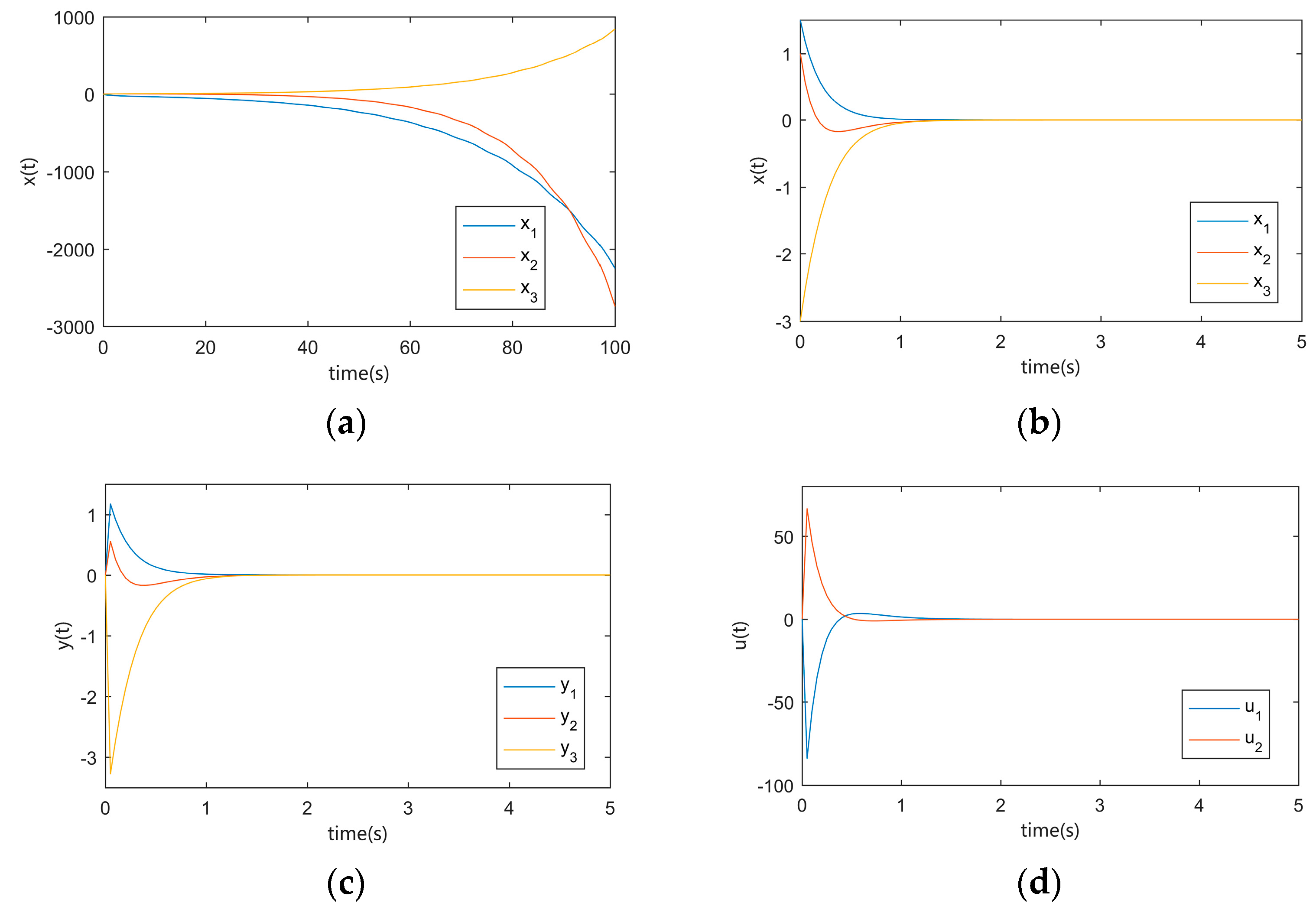
4. Numerical Examples

• Example 1

In this part, the proposed controller design method is applied to the F-404 aircraft engine system [36] to verify the efficacy of the proposed theory. The state space model of system (1) is described as follows:

$$\begin{array}{c}\dot{x}=\left[\begin{array}{ccc}-1.46& 0& 2.428\\ 0.1643+0.5{\beta }_i& -0.4+{\beta }_i& -0.3788\\ 0.3107& 0& -2.23\end{array}\right]x(t)+C_{i}x(t-d_i(t))+\left[\begin{array}{ll}{b}_{11}^i\hfill & b_{12}^i\hfill \\ b_{21}^i\hfill & b_{22}^i\hfill \\ b_{31}^i\hfill & b_{33}^i\hfill \end{array}\right]u+\left[\begin{array}{c}0.1\\ 0.2\\ 0.3\end{array}\right]f(x)\hfill \\ y=D_{i}x(t)\hfill \end{array}$$

where $x\left(t\right)={\left[\begin{array}{ccc}{x}_1^{\mathrm{T}}\left(t\right)& x_2^{\mathrm{T}}\left(t\right)& x_3^{\mathrm{T}}\left(t\right)\end{array}\right]}^{\mathrm{T}}$, with $x_1\left(t\right)$ indicating the sideslip angle, $x_2\left(t\right)$ indicating the roll rate, and $x_3\left(t\right)$ indicating the yaw rate of the F-404 aircraft engine system, respectively. These parameters can be provided in

Table 1. Parameters of the F-404 aircraft engine system model.

Parameters	i = 1	i = 2	i = 3
${\beta }_i$	−0.5	1.5	2
$b_{11}^i$	0.15	0.15	0.15
$b_{12}^i$	0.12	0.2	0.2
$b_{21}^i$	0.15	0.13	0.15
$b_{22}^i$	−1.5	−1.3	−0.15
$b_{31}^i$	0.2	0.3	0.4
$b_{32}^i$	0.2	0.3	0.4

, and the other parameters are offered up as follows:

$$C_i=\left[\begin{array}{ccc}1& 0& 0\\ 0& 1& 0\\ 0& 0& 1\end{array}\right], D_i=\left[\begin{array}{ccc}1& 0& 0\\ 0& 1& 0\\ 0& 0& 1.3\end{array}\right], {\overline{B}}_i=\left[\begin{array}{c}0\\ 1\\ 1\end{array}\right]$$

In order to conveniently employ the conclusions of Theorem 2, the model is transformed into the following three modes of SMJS:

• Mode 1:

$$\begin{array}{c}\dot{x}=\left[\begin{array}{ccc}-1.46& 0& 2.428\\ -0.0857& -0.9& -0.3788\\ 0.3107& 0& -2.23\end{array}\right]x(t)+\left[\begin{array}{ccc}1& 0& 0\\ 0& 1& 0\\ 0& 0& 1\end{array}\right]x(t-d_1(t))+\left[\begin{array}{ll}0.15\hfill & 0.12\hfill \\ 0.15\hfill & -1.5\hfill \\ 0.2\hfill & 0.2\hfill \end{array}\right]u+\left[\begin{array}{c}0.1\\ 0.2\\ 0.3\end{array}\right]f(x)\hfill \\ y=\left[\begin{array}{ccc}1& 0& 0\\ 0& 1& 0\\ 0& 0& 1.3\end{array}\right]x(t)\hfill \end{array}$$

• Mode 2:

$$\begin{array}{c}\dot{x}=\left[\begin{array}{ccc}-1.46& 0& 2.428\\ 0.9143& 1.1& -0.3788\\ 0.3107& 0& -2.23\end{array}\right]x(t)+\left[\begin{array}{ccc}1& 0& 0\\ 0& 1& 0\\ 0& 0& 1\end{array}\right]x(t-d_2(t))+\left[\begin{array}{ll}0.15\hfill & 0.2\hfill \\ 0.13\hfill & -1.3\hfill \\ 0.3\hfill & 0.3\hfill \end{array}\right]u+\left[\begin{array}{c}0.1\\ 0.2\\ 0.3\end{array}\right]f(x)\hfill \\ y=\left[\begin{array}{ccc}1& 0& 0\\ 0& 1& 0\\ 0& 0& 1.3\end{array}\right]x(t)\hfill \end{array}$$

• Mode 3:

$$\begin{array}{c}\dot{x}=\left[\begin{array}{ccc}-1.46& 0& 2.428\\ 1.1643& 1.6& -0.3788\\ 0.3107& 0& -2.23\end{array}\right]x(t)+\left[\begin{array}{ccc}1& 0& 0\\ 0& 1& 0\\ 0& 0& 1\end{array}\right]x(t-d_3(t))+\left[\begin{array}{ll}0.15\hfill & 0.2\hfill \\ 0.15\hfill & -1.5\hfill \\ 0.4\hfill & 0.4\hfill \end{array}\right]u+\left[\begin{array}{c}0.1\\ 0.2\\ 0.3\end{array}\right]f(x)\hfill \\ y=\left[\begin{array}{ccc}1& 0& 0\\ 0& 1& 0\\ 0& 0& 1.3\end{array}\right]x(t)\hfill \end{array}$$

The system jumping modes $\left\{r\left(t\right)\right\}$ are described by the semi-Markov process, and $r\left(t\right)=i\in \left\{1, 2, 3\right\}$. The mode sojourn time will be assumed to follow exponential distributions with the parameters of 1 and 4, respectively, when $i=1, 2$. The last mode sojourn time will be assumed to follow the Weibull distribution with scale parameter and shape parameter of 1 and 2, respectively. Then, the upper and lower bounds for the transition rate are then chosen as follows:

$${\overline{\lambda }}_{ij}=\left[\begin{array}{ccc}-1.5& 0.7& 0.8\\ 0.4& -1& 0.6\\ 0.3& 0.7& -1\end{array}\right], {\underset{\_}{\lambda }}_{ij}=\left[\begin{array}{ccc}-1& 0.3& 0.7\\ 0.2& -0.5& 0.3\\ 0.1& 0.5& -0.6\end{array}\right].$$

The mode-dependent time-varying delays are assumed to be $d_1\left(t\right)=1+0.4\sin \left(t\right)$, $d_2\left(t\right)=1+0.8\sin \left(t\right)$ and $d_3\left(t\right)=1+0.2\cos \left(t\right)$. This gives $h_1=0.2$, $h_2=1.8$, and ${\epsilon }_1=0.5$, ${\epsilon }_2=1$, ${\epsilon }_3=0.5$. It is assumed that the initial state of the system is φ(0) = [1.5 1 3]^T, the initial mode is $r_0=1$ and the system nonlinear parameters are $\alpha =0.01$, $f\left(x\right)=\sigma \sin \left(10t\right)$ and $\sigma =1.1$. Based on Theorem 3, the system can be designed with a static output feedback control law to make the closed-loop system stochastic stable, and the control law gain matrices are obtained as:

$$\begin{gathered} K_1=\left[\begin{array}{lll}-24.7062\hfill & -2.01\hfill & -11.9365\hfill \\ 0.2508\hfill & 2.5334\hfill & -1.2964\hfill \end{array}\right], \\ {K}_2=\left[\begin{array}{lll}-27.7127\hfill & -4.9369\hfill & -6.9075\hfill \\ 2.9157\hfill & 3.6541\hfill & -1.2866\hfill \end{array}\right], \\ {K}_3=\left[\begin{array}{lll}-84.5315\hfill & -47.5973\hfill & -12.745\hfill \\ 37.1042\hfill & 34.5375\hfill & -1.1839\hfill \end{array}\right]. \end{gathered}$$

Figure 1 illustrates the semi-Markov jump mode. The open-loop system trajectory is illustrated in Figure 2a, which shows that the system is instable. By using the designed controller, the state response of the closed-loop system is illustrated in Figure 2b. Figure 2c illustrates the trajectory of the system output, whereas Figure 2d illustrates the trajectory of the control input. It is easily found that the designed controller is effective.

• Example 2

Considering system (1), its parameters are described as follows [37]:

• Mode 1:

$$A_1=\left[\begin{array}{cc}-0.7050& 0.0280\\ 0.0195& -0.6294\end{array}\right], C_1=\left[\begin{array}{cc}0.1& 0\\ 0& 0.2\end{array}\right], F_1=c_1\left[\begin{array}{c}0.1\\ 0.2\end{array}\right],c_1=0.003,$$

• Mode 2:

$$A_2=\left[\begin{array}{cc}-1.1568& 0.0064\\ 0.0434& -1.5905\end{array}\right], C_2=\left[\begin{array}{cc}0.3& 0\\ 0& 0.1\end{array}\right], F_1=c_2\left[\begin{array}{c}0.1\\ 0.2\end{array}\right],c_2=0.011,$$

the other parameters are offered up follows:

$$\begin{array}{c}{B}_i=\left[\begin{array}{c}0.1\\ 0.2\end{array}\right], {\overline{B}}_i=\left[\begin{array}{c}0\\ 1\\ 1\end{array}\right], D_i=\left[\begin{array}{cc}1& 0\\ 0& 1.2\end{array}\right],\hfill \\ d_i\left(t\right)=0.8\left(1-\sin \left(0.5t\right)\right), {\epsilon }_i=1, \alpha =0.01, f\left(x\right)=\sigma \sin \left(t\right), \sigma =0.5.\hfill \end{array}$$

It is assumed that the initial state of the system is $\phi \left(0\right)={\left[\begin{array}{ccc}1.5& 1& 3\end{array}\right]}^{\mathrm{T}}$ and the initial mode is $r_0=1$. From Figure 3b, one can show that the system is stochastic stable and the system state trajectories converge faster compared to that of the literature [37]. Therefore, it can be shown that the stability criterion obtained in this paper is less conservative.

5. Conclusions

In this paper, we discuss the problem of the static output feedback control for nonlinear time-delayed SMJS with an IQC condition. An appropriate mode-dependent Lyapunov–Krasovskii functional is constructed, and a mode-dependent static output feedback control law is designed using the matrix transformation, projection theorem and convex set principle. The feedback control law is given explicitly in the form of LMI, which is convenient for a numerical solution. Finally, the effectiveness and advantages of the proposed method are verified by the F-404 aircraft engine systems and a numerical case. The future works will focus on the analysis and synthesis problems of observer-based time-delayed SMJS with an IQC condition.

References

1. Chavez-Fuentes, J.; Costa, E.; Mayta, J.; Terra, M. Regularity and stability analysis of discrete- time Markov jump linear singular systems. Automatica 2017, 76, 32–40. [Google Scholar] [CrossRef]
2. Feng, X.; Loparo, K.; Ji, Y.; Chizeck, H. Stochastic stability properties of jump linear systems. IEEE Trans. Autom. Control 1992, 37, 38–53. [Google Scholar] [CrossRef]
3. You, K.; Fu, M.; Xie, L. Mean square stability for Kalman filtering with Markovian packet losses. Automatica 2011, 47, 2647–2657. [Google Scholar] [CrossRef]
4. Shi, Y.; Yu, B. Output feedback stabilization of networked control systems with random delays modeled by Markov chains. IEEE Trans. Autom. Control 2009, 54, 1668–1674. [Google Scholar]
5. Wu, N.E. Coverage in fault-tolerant control. Automatica 2004, 40, 537–548. [Google Scholar] [CrossRef]
6. Jacquemart, D.; Morio, J. Conflict probability estimation between aircraft with dynamic importance splitting. Saf. Sci. 2013, 51, 94–100. [Google Scholar] [CrossRef]
7. Cheng, J.; Xie, L.; Park, J.H.; Yan, H. Protocol-based output-feedback control for semi-markov jump systems. IEEE Trans. Autom. Control 2022, 67, 4346–4353. [Google Scholar] [CrossRef]
8. Tian, Y.; Yan, H.; Zhang, H.; Zhan, X.; Peng, Y. Resilient static output feedback control of linear semi-Markov jump systems with incomplete semi-Markov kernel. IEEE Trans. Autom. Control 2020, 66, 4274–4281. [Google Scholar] [CrossRef]
9. Tian, Y.; Yan, H.; Zhang, H.; Cheng, J.; Shen, H. Asynchronous output feedback control of hidden semi-markov jump systems with random mode-dependent delays. IEEE Trans. Autom. Control 2021, 67, 4107–4114. [Google Scholar] [CrossRef]
10. Chen, H.; Zong, G.; Zhao, X.; Gao, F.; Shi, K. Secure filter design of fuzzy switched CPSs with mismatched modes and application: A multi-domain event-triggered strategy. IEEE Trans. Ind. Inform. 2023, 1–10. [Google Scholar] [CrossRef]
11. Zong, G.; Yang, D.; Lam, J.; Song, X. Fault-tolerant control of switched LPV systems: A bumpless transfer approach. IEEE Trans. Mechatron. 2022, 27, 1436–1446. [Google Scholar]
12. Schioler, H.; Leth, J.; Simonsen, M. Stochastic stability of diffusions with semi-Markovian switching. In Proceedings of the 54th IEEE Conference on Decision and Control, Osaka, Japan, 14 December 2015. [Google Scholar]
13. Wang, B.; Zhu, Q. Stability analysis of semi-Markov switched stochastic systems. Automatica 2018, 94, 72–80. [Google Scholar] [CrossRef]
14. Zhang, H.; Qiu, Z.; Xiong, L. Stochastic stability criterion of neutral-type neural networks with additive time-varying delay and uncertain semi-Markov jump. Neurocomputing 2019, 333, 395–406. [Google Scholar] [CrossRef]
15. Shen, H.; Chen, M.; Wu, Z.-G.; Cao, J.; Park, J.H. Reliable event-triggered asynchronous extended passive control for semi-Markov jump fuzzy systems and its application. IEEE Trans. Fuzzy Syst. 2019, 28, 1708–1722. [Google Scholar] [CrossRef]
16. Qi, W.; Park, J.H.; Zong, G.; Cao, J.; Cheng, J. Filter for positive stochastic nonlinear switching systems with phase-type semi-Markov parameters and application. IEEE Trans. Syst. Man Cybern. Syst. 2021, 52, 2225–2236. [Google Scholar] [CrossRef]
17. Wang, J.; Chen, M.; Shen, H. Event-triggered dissipative filtering for networked semi-Markov jump systems and its applications in a mass-spring system model. Nonlinear Dyn. 2017, 87, 2741–2753. [Google Scholar] [CrossRef]
18. Shen, H.; Li, F.; Cao, J.; Wu, Z.G.; Lu, G. Fuzzy-model-based output feedback reliable control for network-based semi-Markov jump nonlinear systems subject to redundant channels. IEEE Trans. Cybern. 2020, 50, 4599–4609. [Google Scholar] [CrossRef] [PubMed]
19. Shen, H.; Li, F.; Cao, J.; Wu, Z.G.; Lu, G. Song. Resilient and robust control for event-triggered uncertain semi-Markov jump systems against stochastic cyber attacks. Int. J. Robust Nonlinear Control 2022, 32, 3847–3871. [Google Scholar]
20. Tian, Y.; Yan, H.; Zhang, H.; Yang, S.X.; Li, Z. Observed-based finite-time control of nonlinear semi-Markovian jump systems with saturation constraint. IEEE Trans. Syst. Man Cybern. Syst. 2020, 51, 6639–6649. [Google Scholar] [CrossRef]
21. Yan, S.; Gu, Z.; Park, J.H.; Xie, X. Adaptive memory-event-triggered static output control of T-S fuzzy wind turbine systems. IEEE Trans. Fuzzy Syst. 2022, 30, 3894–3904. [Google Scholar] [CrossRef]
22. Yang, D.; Zong, G.; Su, S.-F. H tracking control of uncertain Markovian hybrid switching systems: A fuzzy switching dynamic adaptive control approach. IEEE Trans. Cybern. 2022, 66, 3111–3122. [Google Scholar] [CrossRef]
23. Yan, S.; Gu, Z.; Park, J.H.; Xie, X. Distributed-delay-dependent stabilization for networked interval type-2 fuzzy systems with stochastic delay and actuator saturation. IEEE Trans. Syst. Man Cybern. Syst. 2022, 1–11. [Google Scholar] [CrossRef]
24. Yan, S.; Gu, Z.; Park, J.H.; Xie, X. Sampled memory-event-triggered fuzzy load frequency control for wind power systems subject to outliers and transmission delays. IEEE Trans. Cybern. 2022, 1–11. [Google Scholar] [CrossRef]
25. Wu, T.; Xiong, L.; Cao, J.; Zhang, H. Stochastic stability and extended dissipativity analysis for uncertain neutral systems with semi-Markovian jumping parameters via novel free matrix-based integral inequality. Int. J. Robust Nonlinear Control 2019, 29, 2525–2545. [Google Scholar] [CrossRef]
26. Wang, J.; Ma, S.; Zhang, C. Stability analysis and stabilization for nonlinear continuous-time descriptor semi-Markov jump systems. Appl. Math. Comput. 2016, 279, 90–102. [Google Scholar] [CrossRef]
27. Yang, J.; Bu, X.; Yu, Q.; Zhu, F. Observer-based controller design for nonlinear semi-Markov switched system with external disturbance. J. Frankl. Inst. 2020, 357, 8435–8453. [Google Scholar] [CrossRef]
28. Huang, J.; Yu, L.; Chen, L. Control design for stochastic one-sided Lipschitz differential inclusion system with time delay. Int. J. Syst. Sci. 2018, 49, 2923–2939. [Google Scholar] [CrossRef]
29. Açıkmeşe, B.; Corless, M. Observers for systems with nonlinearities satisfying incremental quadratic constraints. Automatica 2011, 47, 1339–1348. [Google Scholar] [CrossRef]
30. Huang, J.; Shi, Y. Stochastic stability and robust stabilization of semi-Markov jump linear systems. Int. J. Robust Nonlinear Control 2013, 23, 2028–2043. [Google Scholar] [CrossRef]
31. Seuret, A.; Gouaisbaut, F. Hierarchy of LMI conditions for the stability analysis of time-delay systems. Systems. Control Lett. 2015, 81, 1–7. [Google Scholar] [CrossRef]
32. Sun, J.; Liu, G.; Chen, J.; Rees, D. Improved delay-range-dependent stability criteria for linear systems with time-varying delays. Automatica 2010, 46, 466–470. [Google Scholar] [CrossRef]
33. Seuret, A.; Gouaisbaut, F.; Fridman, E. Stability of systems with fast-varying delay using improved Wirtinger’s inequality. In Proceedings of the 52th IEEE Conference on Decision and Control, Florence, Italy, 10–13 December 2013. [Google Scholar]
34. Tian, J.; Ma, S.; Zhang, C. Unknown input reduced-order observer design for one-sided Lipschitz nonlinear descriptor Markovian jump systems. Asian J. Control 2019, 21, 952–964. [Google Scholar] [CrossRef]
35. Tuan, H.; Apkarian, P.; Nguyen, T. Robust and reduced-order filtering: New LMI-based characterizations and methods. IEEE Trans. Signal Process. 2001, 49, 2975–2984. [Google Scholar] [CrossRef]
36. Shi, P.; Liu, M.; Zhang, L. Fault-Tolerant Sliding-Mode-Observer Synthesis of Markovian Jump Systems Using Quantized Measurements. IEEE Trans. Ind. Electron. 2015, 62, 5910–5918. [Google Scholar] [CrossRef]
37. Zhang, M.; Huang, J.; Zhang, Y. Stochastic stability analysis of nonlinear semi-Markov jump systems with time delays and incremental quadratic constraints. J. Frankl. Inst. 2021. [Google Scholar] [CrossRef]
Figure 1. Semi-Markov jump modes.
Mca 28 00030 g001
Figure 2. (a) State response of the open-loop system; (b) State response of the closed-loop system; (c) Output response of the closed-loop system; (d) Input response of the closed-loop system.
Mca 28 00030 g002
Figure 3. (a) Semi-Markov jump modes; (b) State response of the closed-loop system.
Mca 28 00030 g003