Article

Mathematical Structure of RelB Dynamics in the NF-κB Non-Canonical Pathway

1
Center for Mathematical Modeling and Data Science, Osaka University, Osaka 565-0871, Japan
2
Consulting Division, Consulting and IT Business Department, Vision Consulting, Inc., Tokyo 106-6139, Japan
*
Author to whom correspondence should be addressed.
Math. Comput. Appl. 2024, 29(4), 62; https://doi.org/10.3390/mca29040062
Submission received: 10 May 2024 / Revised: 25 July 2024 / Accepted: 30 July 2024 / Published: 5 August 2024

Abstract

:
This study analyzed the non-canonical NF-κB pathway, which controls functions distinct from those of the canonical pathway. Although oscillations of NF-κB have been observed in the non-canonical pathway, a detailed mechanism explaining the observed behavior remains elusive, owing to the different behaviors observed across cell types. This study demonstrated that oscillations cannot be produced by the experimentally observed pathway alone, thereby suggesting the existence of an unknown reaction pathway. Assuming this pathway, it became evident that the oscillatory structure of the non-canonical pathway was caused by stable periodic orbits. In addition, we demonstrated that altering the expression levels of specific proteins reproduced various behaviors. By fitting 14 parameters, excluding those measured in previous studies, this study successfully reproduce nuclear retention (saturation), oscillation, and singular events that had been experimentally confirmed. The analysis also provided a comprehensive understanding of the dynamics of the RelB protein and suggested a potential inhibitory role for the unknown factor. These findings indicate that the unknown factor may be an isoform of IκB, contributing to the regulation of NF-κB signaling. Based on these models, we gained invaluable understanding of biological systems, paving the way for the development of new strategies to manipulate specific biological processes.

1. Introduction

The transcription factor NF- κ B influences various cellular functions, including inflammation and immune response [1,2,3,4,5]. The proteins that comprise the NF- κ B family are RelA, RelB, c-Rel, p105/p50, and p100/p52, all of which initiate transcriptional activity through the formation of homo- and heterodimeric complexes [6].
NF- κ B activation is facilitated through two primary signal transduction pathways [7,8], namely the canonical and the non-canonical pathways [9]. The canonical pathway, activated via TNF- α stimulation, regulates the expression of target genes involved in the suppression of apoptosis, cell division, and inflammation [10]. This stimulation results in the NEMO-dependent activation of I κ B kinase (IKK) β , which phosphorylates I κ B α . Consequently, p50/RelA is sequestrated in the cytoplasm, followed by the proteasomal degradation of phosphorylated I κ B α [11,12]. Subsequently, p50/RelA translocates into the nucleus to induce the expression of target genes, including I κ B α itself. As I κ B α is also a target gene, newly synthesized I κ B α results in the export of p50/RelA to the cytoplasm. p50/RelA is shuttled between the nucleus and cytoplasm through repetitions of the above process. This nucleus–cytoplasm (N-C) oscillation facilitates proper functional control [13,14]. Focusing on canonical pathways, Hatanaka et al. constructed a new mathematical model of NF- κ B activation to explore the modulation of the oscillation based on the phosphorylation of I κ B α and RelA. Through a stability analysis around the equilibrium point, they confirmed that I κ B α phosphorylation resulted in the addition of a structure with a stable periodic solution to the phosphorylation model [15]. However, Hoffmann et al. generated cell lines lacking individual and multiple NF κ B proteins and used them to establish interactions between components of the NF κ B-I κ B signaling system [16].
Non-canonical pathways are activated via lymphotoxin (LT) stimulation and induce the expression of target genes involved in the formation and maintenance of lymphoid organs and the maturation of lymphocytes [17]. NF- κ B-inducing kinase (NIK), activated via LT stimulation, yields phosphorylated IKK α . The activated IKK α phosphorylates p100 of p100/RelB and triggers partial proteolysis of p100/RelB to p52/RelB. Consequently, p52/RelB translocates into the nucleus and induces the transcription of its target genes [18].
Typically, the detailed mechanism of the non-canonical pathway remains elusive compared to the canonical pathway. However, recently, N-C oscillations of RelB similar to the canonical pathway have been reported [19]. In RelB fluorescence experiments, the N-C oscillation of RelB was confirmed in the case of LT stimulation input. However, in the non-canonical pathway, RelB oscillation was observed in only approximately 40% of the cells. In 30% of the remaining cells, RelB gradually accumulated in the nucleus (nuclear retention), and in another 10% of the cells, RelB translocated to the nucleus once, then returned to the cytoplasm (singular event). The remaining 20% did not respond to the stimulus ([20]—Figure 13A).
Furthermore, knockout experiments of I κ B α and p100 have shown that I κ B α is essential for RelB cytoplasmic translocation and that p100 suppresses RelB oscillation [20]. In I κ B α knockout experiments, nuclear export of p52/RelB was suppressed. Moreover, p100 knockout experiments have indicated that RelB oscillates automatically, even in the absence of LT stimulation. Thus, these results predict that RelB originally has a unique mechanism for self-sustaining oscillation via I κ B α and that the oscillation is suppressed by p100. In the case of the non-canonical pathway, studies of the time evolutions of the nuclear/total ratio have been conducted to reproduce nuclear retention (saturation), oscillation, and singular events. However, these parameters were determined through parameter-fitting to reproduce these three types of RelB dynamics. Consequently, the parameters exhibit discrepancies relative to the values reported in other previous research.
This study elucidated the fundamental mechanism of N-C oscillation in non-canonical pathways and, consequently, clarified the change in behavior from cell to cell. First, we constructed a p100 knockout model to clarify the structure of RelB self-sustained oscillation based on the dynamical system theory. Thereafter, through the addition of a pathway for p100 to the p100 knockout model, we extended it to a model including all pathways of the non-canonical pathway. Consequently, the cause of the different behavior of RelB in each cell was analyzed through a numerical simulation. Furthermore, we calibrated a set of parameters that reproduced the three types of RelB dynamics while setting the parameters to the values reported in previous studies. For the calibration of the parameter set, there are methods of identifying the probability density function (PDF) through sensitivity analysis [21], as well as the hybrid model proposed in a case study of the NF κ B signaling pathway [22]. However, in this study, for simplicity, we explored a set of constant parameters using sensitivity analysis.

2. Materials and Methods
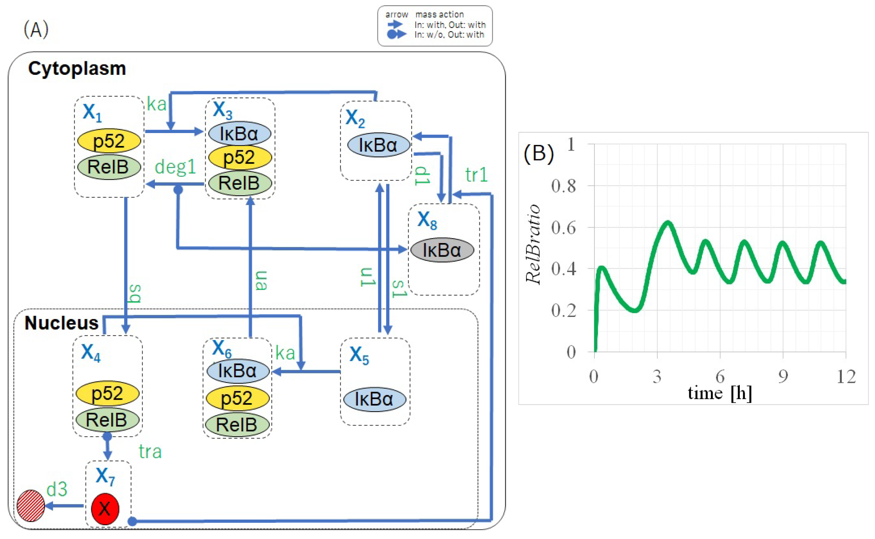
We assigned the variables X 1 , X 2 , , X 14 to represent the concentrations of molecules in the p100 knockout model (p100KO-M) and the non-canonical pathway full model (NC-FM), which are discussed later, as defined in Table 1.

2.1. Negative Feedback from I κ B α Is Essential for the Self-Sustained Oscillation of RelB

To analyze the mechanism of RelB self-sustained oscillations, a mathematical model was constructed based on experimental results. In this model, RelB formed a dimer with p50, owing to the p100 knockout. The p100 knockout model primarily comprises p50/RelB and I κ B α , where each protein translocates from the cytoplasm to the nucleus independently. p50/RelB itself can be exported from the cytoplasm to the nucleus; however, I κ B α mediates to facilitate export from the nucleus to the cytoplasm. I κ B α can shuttle between the cytoplasm and nucleus. Moreover, I κ B α is decomposed from cytoplasmic I κ B α /p50/RelB at a constant rate (Table 2).
RelB did not oscillate automatically in models constructed using pathways (i) to (iv), as shown in Table 2. This absence of oscillation is attributable to the lack of a feedback loop from nuclear p50/RelB to cytoplasmic I κ B α . Therefore, the following pathways were assumed as the feedback loop from nuclear p50/RelB to I κ B α . Consequently, a model was constructed as follows.
  • (a) Certain elements activated via nuclear p50/RelB switched the activation state of I κ B α (i.e., whether I κ B α can bind to RelB).
A model that includes pathways (i) to (iv) and assumption (a) is referred to as p100KO-M. This is expressed through the following simultaneous ordinary differential equations.
(1a) d X 1 d t = s q X 1 + d e g 1 X 3 k a X 1 X 2 , (1b) d X 2 d t = ( d 1 + s 1 ) X 2 + u 1 X 5 + t r 1 X 7 X 8 k a X 1 X 2 , (1c) d X 3 d t = d e g 1 X 3 + u a X 6 + k a X 1 X 2 , (1d) d X 4 d t = s q X 1 k a X 4 X 5 , (1e) d X 5 d t = s 1 X 2 u 1 X 5 k a X 4 X 5 , (1f) d X 6 d t = u a X 6 + k a X 4 X 5 , (1g) d X 7 d t = t r a X 4 d 3 X 7 , (1h) d X 8 d t = d 1 X 2 + d e g 1 X 3 t r 1 X 8 .
We reduced p100KO-M to a reduced model with 6 ordinary differential equations and 2 conservation laws as follows.
(2a) d X 1 d t = s q X 1 + d e g 1 X 3 k a X 1 X 2 , (2b) d X 2 d t = ( d 1 + s 1 ) X 2 + u 1 X 5 + t r 1 X 7 X 8 k a X 1 X 2 , (2c) X 3 = t o t a l R e l B X 1 X 4 X 6 , (2d) d X 4 d t = s q X 1 k a X 4 X 5 , (2e) d X 5 d t = s 1 X 2 u 1 X 5 k a X 4 X 5 , (2f) d X 6 d t = u a X 6 + k a X 4 X 5 , (2g) d X 7 d t = t r a X 4 d 3 X 7 , (2h) X 8 = t o t a l I κ B α t o t a l R e l B + X 1 X 2 + X 4 X 5 .
Then, the following nitial conditions were applied to differential Equation (2):
X 1 , X 2 , X 4 , X 5 , , X 7 = 0 ,
followed by the calculation of the time evolutions of X 1 X 8 .Here, we define R e l B r a t i o as the ratio of RelB within the nucleus to t o t a l R e l B as follows.
R e l B r a t i o = X 4 + X 6 t o t a l R e l B .
In p100KO-M, the degradation of I κ B α is necessary. Rather, I κ B α must enter an inactive state, wherein it cannot bind to the p50/RelB complex, as illustrated in Figure 1A. The unknown factor assumed in hypothesis (a) activated I κ B α and promoted binding to p50/RelB. I κ B α was assumed to be inactivated at a constant rate by a certain factor. As I κ B α is considered to have both activated and inactivated states, p100KO-M contained the equation for inactive I κ B α .
The self-sustained oscillation of RelB can be obtained by setting the parameters appropriately in p100KO-M. The parameters of Partially Numerically Adjusted Values (PAVs) presented in Table 3 were calibrated such that the period of RelB was 1.85 h, as estimated by the experimental values [20]. The time evolution shown in Figure 1B exhibits the oscillation of RelB in the p100 knockout model, which is suggested to exist as a stable periodic orbit generated by the feedback loop of p50/RelB and I κ B α . The unknown pathway constituting the feedback loop from p50/RelB to I κ B α suggested in this section is an essential factor for facilitating the self-sustained oscillation of RelB. Therefore, in the next section, we extend p100KO-M to a model including the entire non-canonical pathway.

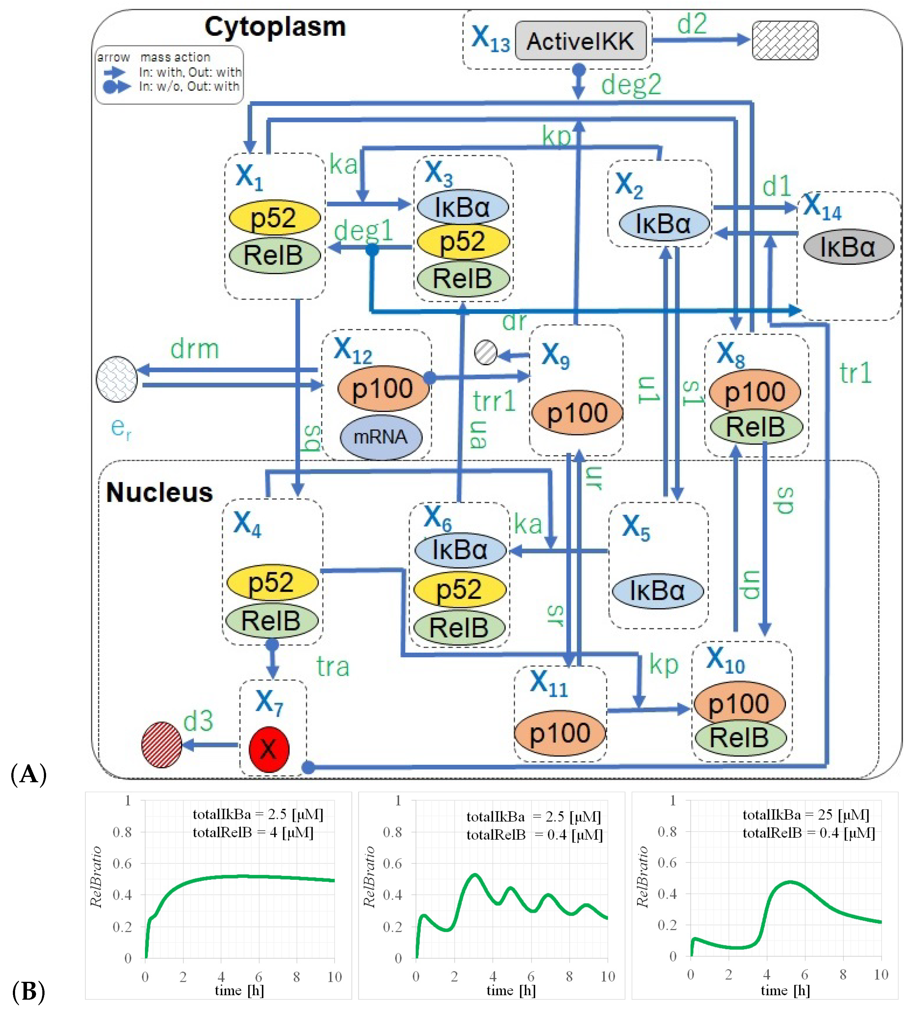
2.2. Full Non-Canonical Pathway Model

To analyze the three types of dynamics of RelB observed in response to LT stimulation, p100KO-M was extended through the addition of a pathway related to p100. Herein, p100 was bound to RelB in the unstimulated state. IKK activated through LT stimulation phosphorylated p100 and induced partial degradation to p52/RelB. p100 was supplied from outside the system, and p100 could move between the cytoplasm and nucleus. When p100 came in contact with p52/RelB in the cytoplasm or nucleus, p52/RelB replaced p100/RelB (Figure 2A). The model wherein p100 was added to p100KO-M is referred to as NC-FM (Equation (5)).
As the extended models included the p100 knockout model, they exhibited an oscillating structure. Therefore, we considered the oscillatory state to be the basic state and set the parameters accordingly. The parameters were set to the same values as for the p100 knockout model. The remaining parameters were set such that 4 or 5 peaks were formed, as in the experimental results of the oscillation event presented in Figure 3, which show three types of RelB dynamics, namely nuclear retention (saturation), oscillation, and singular events. The experimental methods are described in detail in Appendix C. As p100/RelB was localized in the cytoplasm when unstimulated, the parameter of p100 translocation from the nucleus to the cytoplasm was set as greater than that from the cytoplasm to the nucleus. Moreover, the coefficient of reaction wherein p100 and p52 were replaced was set to be larger than the binding coefficient of I κ B α and p52/RelB.
Subsequently, to investigate the appearance of the other two states, namely nuclear retention and singular events, we analyzed the structure of the equation of oscillatory states. As indicated by the results of the sensitivity analysis for t o t a l R e l B and t o t a l I κ B α , the time evolutions shown in Figure 2B in the NC-FM reproduced the transitions from oscillatory states to nuclear retention and singular events. In the NC-FM, with an increase in the t o t a l R e l B , the RelB behavior gradually changed to nuclear retention, whereas, with an increase in the t o t a l I κ B α , the RelB behavior changed to a singular event. This is because a change in the amount of RelB or I κ B α enhanced the translocation of RelB to the nucleus or the cytoplasm, and the oscillatory state became unbalanced.
The NC-FM can be expressed by the following simultaneous equations.
(5a) d X 1 d t = s q X 1 + d e g 1 X 3 k a X 1 X 2 k p X 1 X 9 + d e g 2 X 13 X 8 , (5b) d X 2 d t = ( d 1 + s 1 ) X 2 + u 1 X 5 + t r 1 X 7 X 14 k a X 1 X 2 , (5c) d X 3 d t = d e g 1 X 3 + u a X 6 + k a X 1 X 2 , (5d) d X 4 d t = s q X 1 k a X 4 X 5 k p X 4 X 11 , (5e) d X 5 d t = s 1 X 2 u 1 X 5 k a X 4 X 5 , (5f) d X 6 d t = u a X 6 + k a X 4 X 5 , (5g) d X 7 d t = t r a X 4 d 3 X 7 , (5h) d X 8 d t = ( d e g 2 X 13 + s p ) X 8 + u p X 10 + k p X 1 X 9 , (5i) d X 9 d t = ( s r + d r ) X 9 + u r X 11 + t r r 1 X 12 k p X 1 X 9 , (5j) d X 10 d t = s p X 8 u p X 10 + k p X 4 X 11 (5k) d X 11 d t = s r X 9 u r X 11 k p X 4 X 11 , (5l) d X 12 d t = e r d r m X 12 , (5m) d X 13 d t = d 2 X 13 , (5n) d X 14 d t = d 1 X 2 + d e g 1 X 3 t r 1 X 7 X 14 .
We can reduce the NC-FM to a reduced model with 12 ordinary differential equations and 2 conservation laws as follows.
(6a) d X 1 d t = s q X 1 + d e g 1 X 3 k a X 1 X 2 k p X 1 X 9 + d e g 2 X 13 X 8 , (6b) d X 2 d t = ( d 1 + s 1 ) X 2 + u 1 X 5 + t r 1 X 7 X 14 k a X 1 X 2 , (6c) d X 3 d t = d e g 1 X 3 + u a X 6 + k a X 1 X 2 , (6d) d X 4 d t = s q X 1 k a X 4 X 5 k p X 4 X 11 , (6e) d X 5 d t = s 1 X 2 u 1 X 5 k a X 4 X 5 , (6f) d X 6 d t = u a X 6 + k a X 4 X 5 , (6g) d X 7 d t = t r a X 4 d 3 X 7 , (6h) d X 8 d t = ( d e g 2 X 13 + s p ) X 8 + u p X 10 + k p X 1 X 9 , (6i) d X 9 d t = ( s r + d r ) X 9 + u r X 11 + t r r 1 X 12 k p X 1 X 9 , (6j) X 10 = t o t a l R e l B X 1 X 3 X 4 X 6 X 8 (6k) d X 11 d t = s r X 9 u r X 11 k p X 4 X 11 , (6l) d X 12 d t = e r d r m X 12 , (6m) d X 13 d t = d 2 X 13 , (6n) X 14 = t o t a l I κ B α X 2 X 3 X 5 X 6 .
Through the application of initial conditions of
(7a) X 8 = t o t a l R e l B , (7b) X 13 = a c t i v e I K K , (7c) X 14 = t o t a l I κ B α , (7d) X 1 , X 2 , , X 7 , X 9 , X 11 , X 12 , X 13 = 0 ,
to differential Equation (6), followed by the calculation of the time evolutions of X 1 X 14 , the R e l B r a t i o is obtained as
R e l B r a t i o = X 4 + X 6 + X 10 X 1 + X 3 + X 4 + X 6 + X 8 + X 10 .

3. Results

3.1. Parameter Calibrations

We set the parameters based on previous studies [13,23,24], as indicated by the values presented in Table 3. Owing to the lack of any published data for t r a , it was set such that the three types of RelB dynamics could be observed. An analysis of which parameters of the PAVs in Table 3 significantly differed from the experimenter’s estimates and experimentally measured values (EMVs) is presented in Section 4.

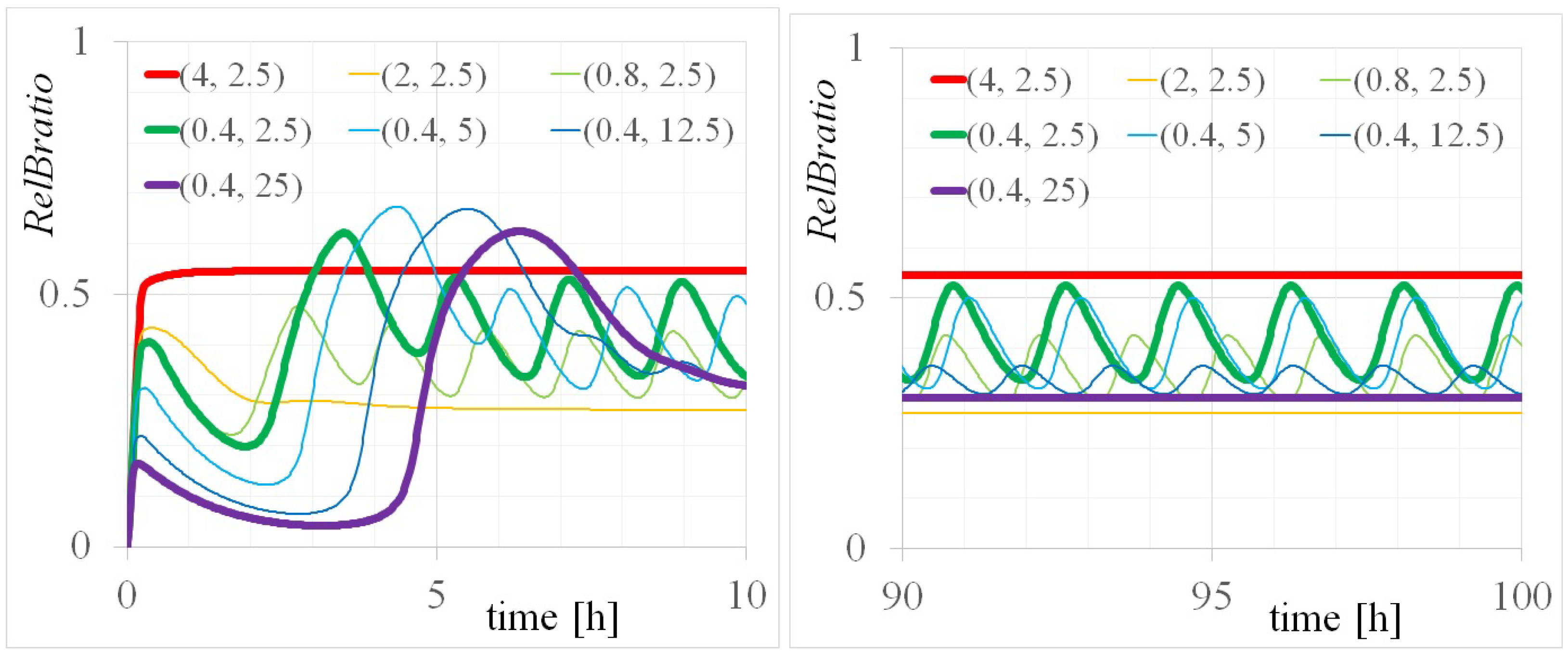
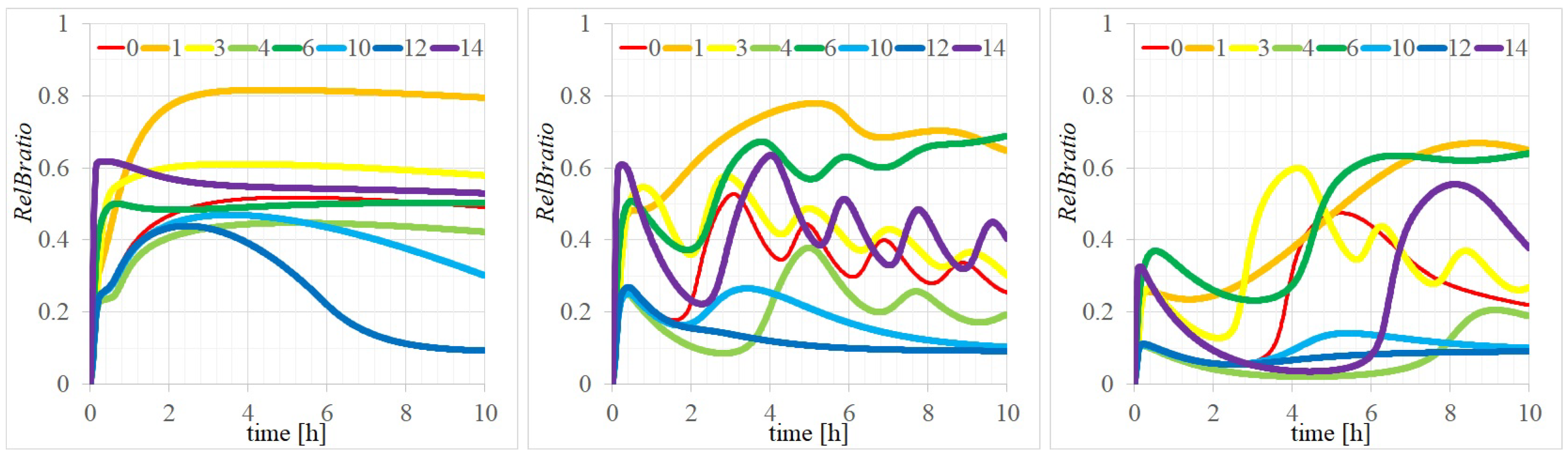
3.2. Three Types of RelB Dynamics Are Dependent on the Concentrations of Total t o t a l I κ B α and t o t a l R e l B

To investigate the transitions to the other two states, namely from the oscillation state to nuclear retention and the singular event, the structure of the equation for the oscillation events was analyzed. This analysis focused on the stability of the equilibrium point of the NC-FM. It was found that the oscillation in the non-canonical pathway was attributable to a stable periodic orbit that transiently appeared along with the decay of active IKK. This mirrored the behavior observed in the canonical pathway model. Thus, RelB oscillation exhibited consistent behavior in cells with identical parameters. Consequently, the appearance of behaviors diverging from the oscillatory state necessitated variability in the parameters across different cells.
A sensitivity analysis was conducted to examine the effect of the changes in parameters on the RelB dynamics. In particular, we focused on the total amounts of RelB and I κ B α . This emphasis was owing to the observation that protein concentrations were more variable across cells than the reaction coefficients, which were determined based on protein types. Notably, t o t a l I κ B α is only relevant in the context of the NC-FM. By conducting a sensitivity analysis of t o t a l R e l B and t o t a l I κ B α in the NC-FM, we successfully replicated both the nuclear retention and singular events, as shown in Figure 2B.
We evaluated the time evolutions of R e l B r a t i o considering the parameters of t o t a l I κ B α and t o t a l R e l B by calculating Equation (8), as shown in Figure 2B. The parameters were set as indicated by the values in Table 3, with values of ( t o t a l R e l B , t o t a l I κ B α ) = (left) (4, 2.5), (center) (0.4, 2.5), and (right) (0.4, 25) [ μ M].
The time evolutions of the RelB ratio (red lines in Figure 2B) indicate the oscillation events at various concentrations of t o t a l R e l B and t o t a l I κ B a , where Figure 2 (left), (center), and (right) correspond to saturation (nuclear retention), oscillation, and singular events, respectively. The trend of characteristic changes in these three events can be interpreted as being correctly reproduced. In the NC-FM, the deviations in t o t a l I κ B α and t o t a l R e l B from their original values facilitated transitions from the oscillation state to a singular event and nuclear retention, respectively. This shift was attributed to the alterations in the amounts of RelB or I κ B α , which enhanced the translocation of RelB to either the nucleus or the cytoplasm. Consequently, the balance of the oscillatory state was disrupted. Quantitatively, by adjusting t o t a l R e l B or t o t a l I κ B α to 10 times, as shown in Figure 2B, the oscillation events were changed to saturation and singular events, respectively.

4. Discussion

This study constructed the p100KO-M and full pathway models for the NF- κ B non-canonical pathway and mathematically analyzed the mechanism of RelB N-C oscillation. Analysis of the p100KO-M model revealed that the pathway connecting p50/RelB and I κ B α was essential for achieving self-sustained RelB oscillation. Consequently, we proposed two pathways from p50/RelB to I κ B α , namely the transcriptional induction of I κ B α by p50/RelB and that of an unknown factor that promoted the binding of I κ B α and RelB by p50/RelB.
The transcription rate of this unknown factor, represented by e r , was determined to be e r = 10−3 [ μ M/min] by fitting to experimental results [20] related to the time evolution during oscillatory events. However, the values of e r from literature data, specifically 1.9 × 10 7 [ μ M/min] [24] and 3 × 10 8 [ μ M/min] [23] for the transcription rate for p100 mRNA, indicated a discrepancy of approximately four orders of magnitude compared to our findings. Despite this significant variance in the e r values, the temporal evolutions depicted in Figure 4 related to these values did not exhibit notable differences. Sensitivity analysis based on the results presented in Figure 4 suggested a complex pathway for the unknown factor.
RelB oscillation was attributed to a stable periodic orbit, with its appearance range controlled by the amounts of RelB and I κ B α . As p100KO-M was incorporated within the full pathway model, the oscillatory state was considered the baseline. Moreover, the other states of nuclear retention and singular events were expressed by the difference in parameters for each cell. Notably, in the NC-FM, nuclear retention and singular events were observed owing to variations in t o t a l R e l B and t o t a l I κ B α levels, respectively, which corresponded to the range wherein the stable periodic orbit was absent in p100KO-M.
Parameter changes beyond t o t a l R e l B and t o t a l I κ B α also confirmed certain differences in the behavior of RelB. This suggested that parameters associated with translocation and transcription may vary with cell size or the cytoplasm-to-nucleus size ratio. However, as reactions such as binding and translocation are protein-specific, the primary variables influencing the dynamics of RelB were t o t a l R e l B and t o t a l I κ B α .

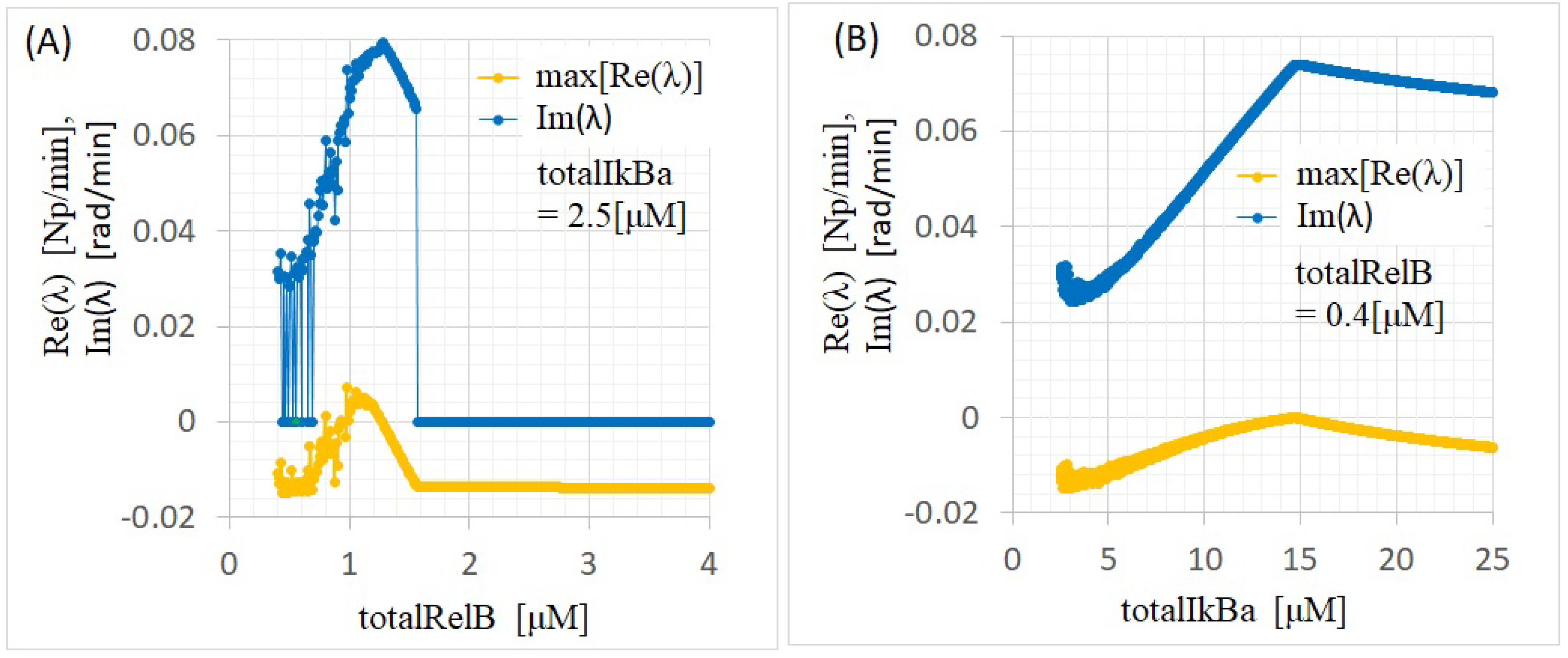
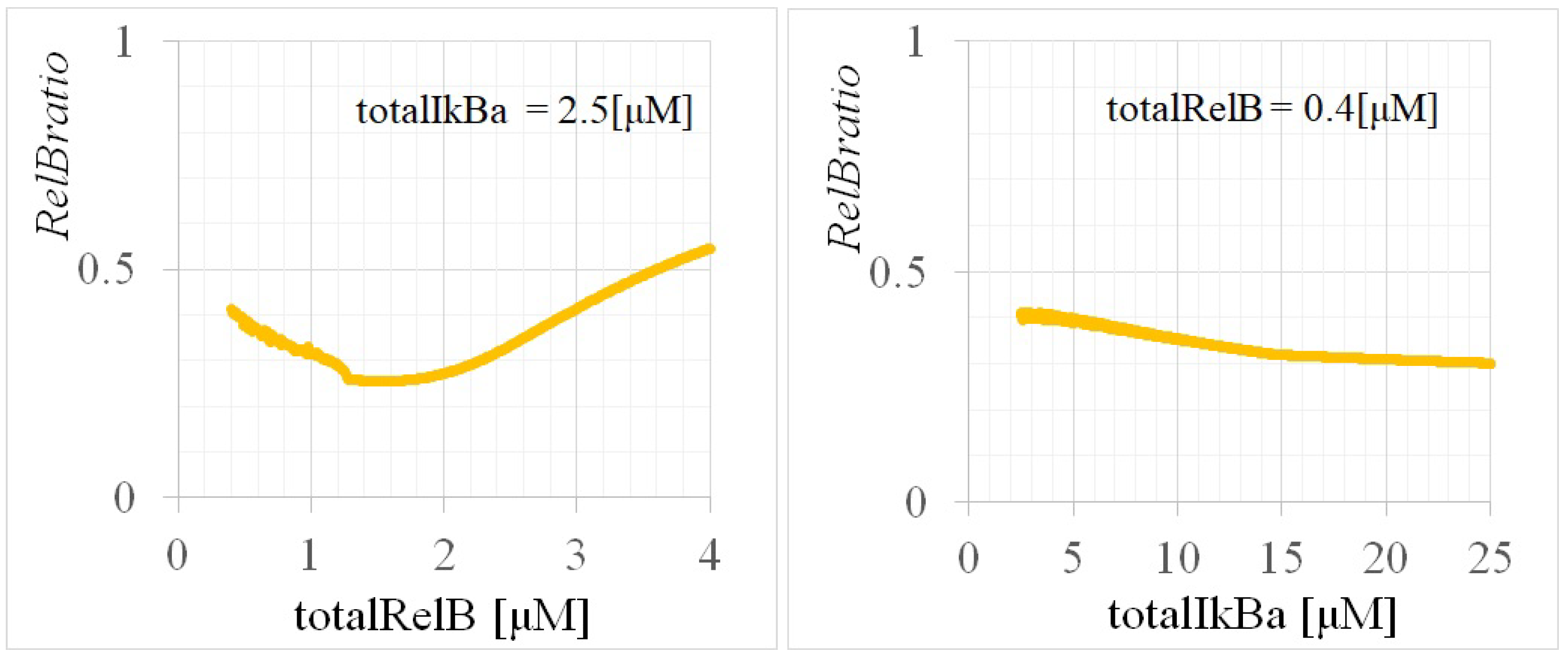
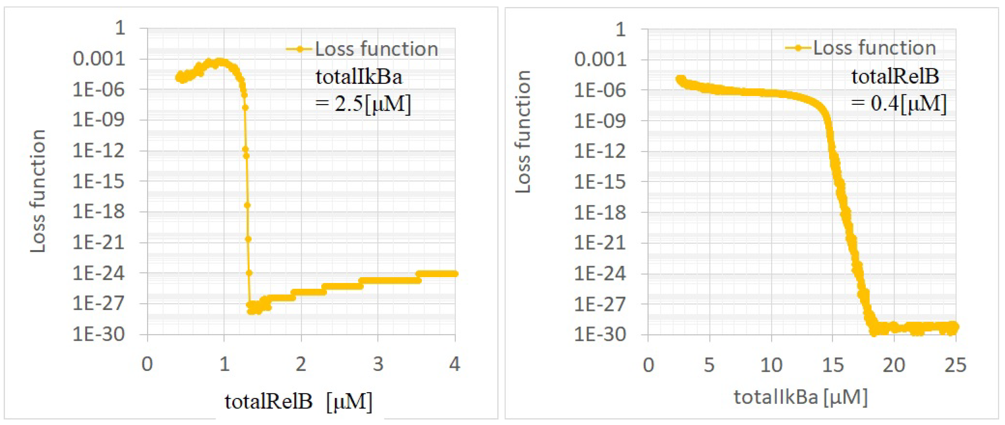
4.1. Dependency of RelB Dynamics on Concentrations of t o t a l R e l B and t o t a l I κ B α

In Section 2.2, we detailed the calculation results using the NC-FM and observed three distinct events in the time evolution of the RelB ratio across various levels of t o t a l R e l B and t o t a l I κ B α . These calculation results, which closely matched the experimental data shown in Figure 2, utilized the PAVs listed in Table 4. However, when the parameters were set to their experimentally measured values (EMVs), the simulation failed to replicate the observed R e l B r a t i o dynamics. The parameters in question included the following fourteen distinct values: (1) s q , (2) k a , (3) t r a , (4) d e g 1 , (5) k p , (6) s p , (7) u p , (8) s r , (9) u r , (10) t r r 1 , (11) d r , (12) d r m , (13) e r , and (14) d e g 2 .
We analyzed the effects of varying these parameters on the time evolution of R e l B r a t i o . The results for all fourteen parameters are presented in Appendix A. In particular, variances in the R e l B r a t i o time evolutions for parameters (1) s q , (3) t r a (4) d e g 1 , (6) s p , (10) t r r 1 , (12) d r m , and (14) d e g 2 , highlighted by thick lines in Figure 5, demonstrated significant deviations from the baseline (represented by the medium red line), particularly for configurations of ( t o t a l R e l B , t o t a l I κ B α ) at (left) (4, 2.5), (center) (0.4, 2.5), and (right) (0.4, 25) [ μ M]. Legends 0–14 correspond to the scenarios wherein parameters were set to PAVs or one of the EMVs.
Further examination of the seven parameters exhibiting substantial time evolution differences between PAV and EMV settings revealed that most discrepancies, such as those for s q = 0.2, 5.4 [1/min], d e g 1 = 0.1, 0.032 [1/min], s p = 0.001, 0.028 [1/min], t r r 1 = 0.1, 0.5 [1/min], and d e g 2 = 0.5, 4.2 [1/ μ M min], with values within an acceptable one-order magnitude range. The variance for t r a = 0.1 and 0.01 [ μ M/min], attributable to the transition speed of an unknown factor, also remained within a permissible range. However, the difference observed for d r m = 0.1, 0.0016 [1/min], spanning two orders of magnitude, indicates the involvement of a complex pathway for its estimated value.
This study performed sensitivity analysis for individual parameters. Future research, by leveraging quantitative data on protein expression levels across various cells, could enhance the reproduction of RelB behavior via adjustments to multiple parameters simultaneously. This approach may also further elucidate the control mechanisms that govern non-canonical pathways, necessitating additional considerations for parameter-set calibration.

4.2. Quantitative Consideration of the Formation of X 1 , X 2 , , X 14

In terms of the p100KO model, we present detailed explanations about the potential of the RelB-p52 complex ( X 1 , X 4 ) in Figure 6 to induce the expression of endogenous I κ B α ( X 3 , X 6 ). Specifically, to quantitatively examine the temporal evolution of X i , by comparing the temporal evolution of ( X 1 , X 4 ) and ( X 3 , X 6 ), it can be observed that ( X 2 , X 5 ) appears after the decline and rise of ( X 3 , X 6 ), respectively. To address the question of whether the unknown protein ( X 7 ) plays a similar role to I κ B α ( X 2 , X 5 ), we compared the temporal evolution of X 7 (bottom right of Figure 6) with that of ( X 2 , X 5 ) (bottom left of the same figure). The similarity of the observed waveforms suggests that X 7 may, indeed, play a similar role. Regarding the similarity of I κ B α and the RelB-p52 complex, comparing the temporal evolutions of ( X 2 , X 5 ) and ( X 1 , X 4 ) in Figure 6 reveals that the times of the maxima and minima in the two waveforms are remarkably similar. It can also be observed that the amplitudes of ( X 1 , X 4 ) are suppressed following each maximum. Regarding the similarity of I κ B α and the RelB-p52 complex, comparing the temporal evolution of ( X 2 , X 5 ) and ( X 1 , X 4 ) in Figure 6 reveals that the times of the maxima and minima in the two waveforms are remarkably similar to those of p100KO model. It can also be observed that the amplitudes of ( X 1 , X 4 ) are suppressed following each maximum.
In terms of the NC-FM, we present detailed explanations about X i in Figure 7. The time evolutions of p100 ( X 9 , X 11 ) are similar to those of I κ B α ( X 2 , X 5 ), with X 9 increasing as shown in the center-left and lower panels of Figure 7. p100-mRNA X 12 is almost constant at 0.01 μ M after 1 h. Regarding the similarity of I κ B α and the RelB-p52 complex, comparing the temporal evolution of ( X 2 , X 5 ) and ( X 1 , X 4 ) in Figure 7 reveals that the times of the maxima and minima in the two waveforms are remarkably similar. It can also be observed that the amplitudes of ( X 1 , X 4 ) are suppressed following each maximum. This suppression may suggest low affinity between I κ B α and the RelB-p52 complex [25,26].
Analysis of the p100KO-M and NC-FM models indicated the presence of a regulatory component analogous to I κ B, represented by the variable X 7 . The temporal evolution of X 7 , particularly in the NC-FM model, mirrors the behavior observed in other I κ B isoforms, as evidenced by the waveform similarities in the middle-left and middle-right panels of Figure 7. These findings suggest that X 7 could play a role in the non-canonical NF- κ B signaling pathway similar to that of I κ B, acting as an inhibitory regulator by interacting with components such as RelB. The consistent suppression observed in the amplitudes of X 1 and X 4 following the maxima further supports the hypothesis that X 7 may have an inhibitory function, possibly through sequestration of RelB complexes. Given these observations, it is plausible that X 7 represents an isoform of I κ B. This hypothesis aligns with the need for a negative regulatory mechanism to maintain homeostasis in the NF- κ B signaling pathways.
Further empirical studies are recommended to conclusively identify X 7 . Investigating the molecular identity of X 7 and its interactions with NF- κ B components will be crucial for understanding its precise role and for potentially classifying it as a new member of the I κ B family.

5. Conclusions

Using the p100KO-M and the NC-FM, this study established mathematical frameworks for analyzing the self-sustained oscillation of RelB and its dynamics in response to LT stimulation. Our investigation highlighted the critical roles of protein translocation between the nucleus and cytoplasm, feedback loops, and specific protein interactions in the dynamic responses of cells. Furthermore, numerical analysis revealed variability in the oscillatory behavior of RelB and cell-to-cell behavior under certain parameter conditions. We identified the following three distinct types of RelB dynamics: saturation (nuclear retention), oscillation, and singular events. By adjusting the values of t o t a l R e l B and t o t a l I κ B α to 10 times those obtained in the oscillation events, we were able to replicate the saturation and singular events, respectively. This replication employed 14 parameters with PAVs that were corrected from EMVs. Significant variance in the time dependencies of the RelB ratio were observed for parameters s q , d e g 1 , s p , t r r 1 , d e g 2 , e r , and d r m , indicating influences of unknown factors. Bifurcation analysis using a simplified KO model highlighted the proposed model’s ability to predict system behaviors, pinpointing critical transitions between three different system states, namely saturation, oscillation, and singular events, and providing insights into the mechanisms driving these changes. Despite certain simplifications of the full model, the analysis confirmed the model’s effectiveness and its potential application in further complex system studies. This study provided a comprehensive analysis of the NF- κ B non-canonical pathway, focusing on the dynamics of the RelB protein and the potential role of X 7 as an inhibitory factor. The findings suggest that X 7 may, indeed, be an isoform of I κ B, contributing to the regulation of NF- κ B signaling. Based on these models, we gained invaluable understanding of biological systems, paving the way for the development of new strategies to manipulate specific biological processes.

Author Contributions

Conceptualization, T.U., N.H. and T.S.; methodology, T.U., N.H. and T.S.; software, T.U. and N.H.; validation, T.U., N.H. and T.S.; formal analysis, T.U. and N.H.; investigation, T.U., N.H. and T.S.; resources, T.U. and N.H.; data curation, T.U. and N.H.; writing—original draft preparation, T.U.; writing—review and editing, T.U., N.H. and T.S.; visualization, T.U. and N.H.; supervision, T.S.; project administration, T.S.; funding acquisition, T.S. All authors have read and agreed to the published version of the manuscript.

Funding

This research was funded by JST, CREST Grant Number JPMJCR2022, Japan.

Data Availability Statement

The data presented in this study are available on request from the corresponding author.

Acknowledgments

We would like to express our sincere gratitude to Reviewers 1 and 2 for their insightful comments and constructive feedback on our manuscript. Their valuable suggestions significantly contributed to the improvement and clarity of our work. We deeply appreciate their time and effort in reviewing our paper and helping us enhance the quality of our research.

Conflicts of Interest

The authors declare no conflict of interest. The authors declare that the research was conducted in the absence of any commercial or financial relationships from Vision Consulting, Inc. that could be construed as a potential conflict of interest.

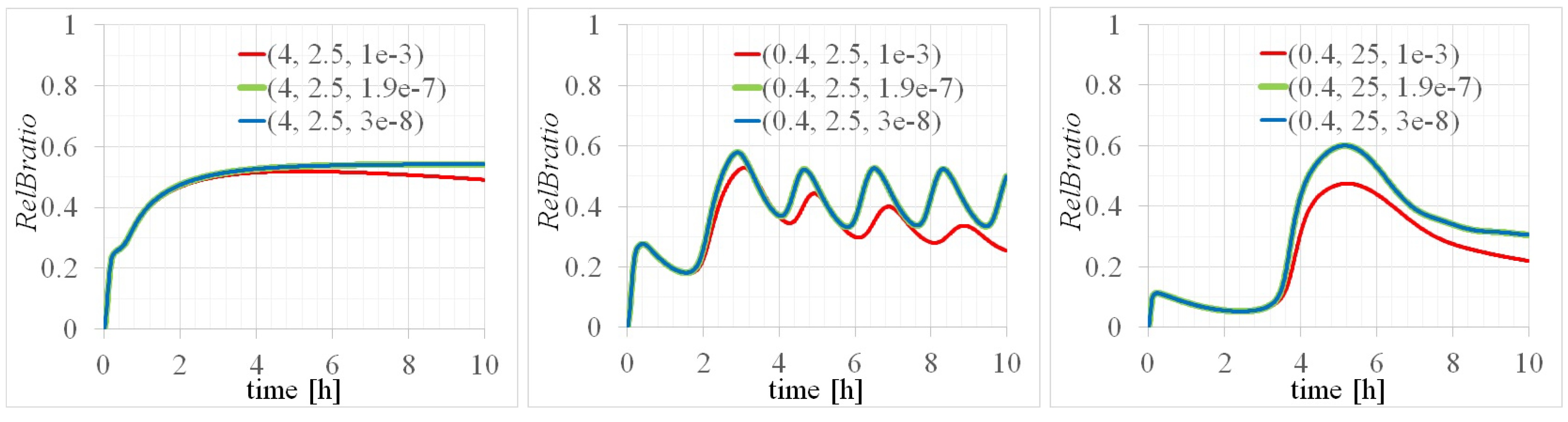
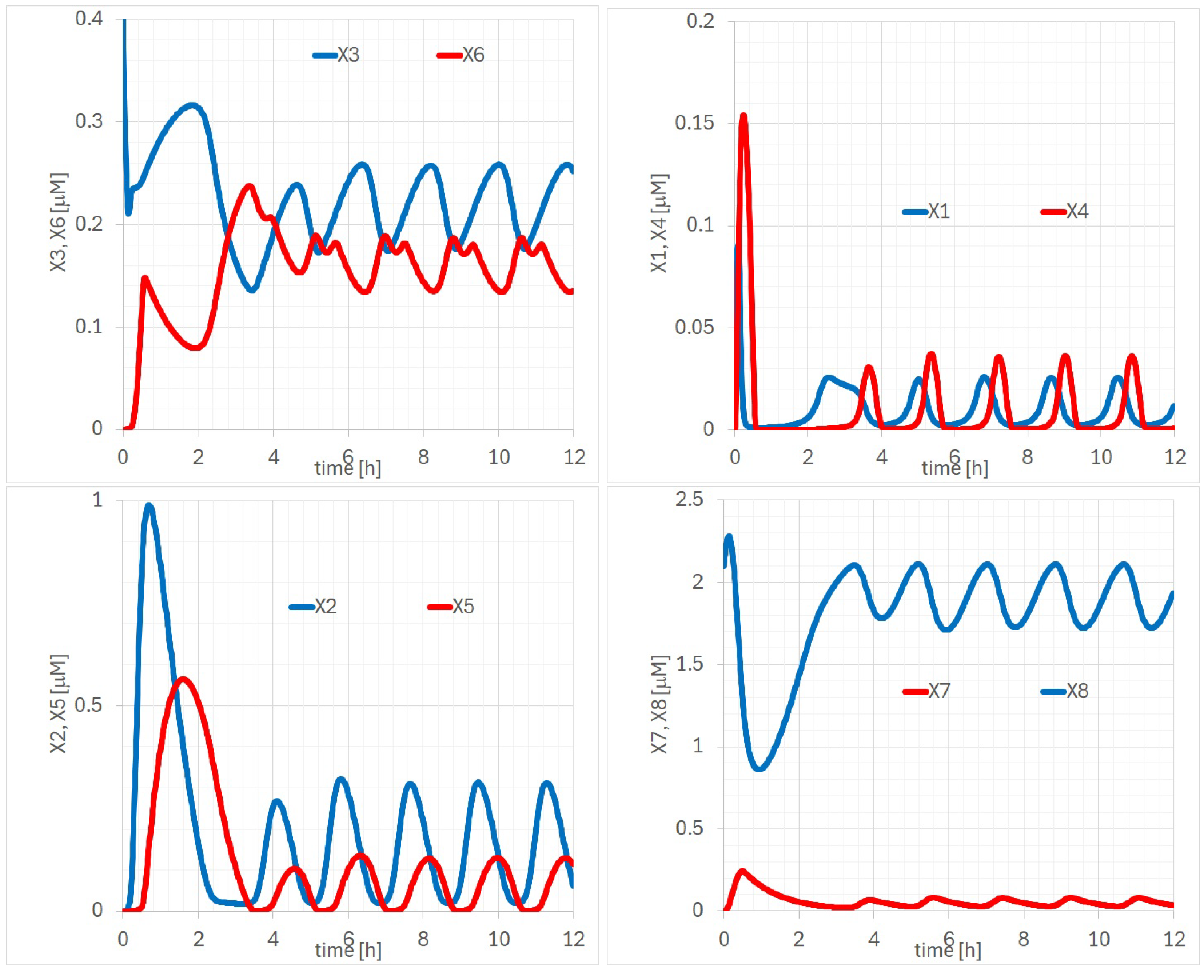
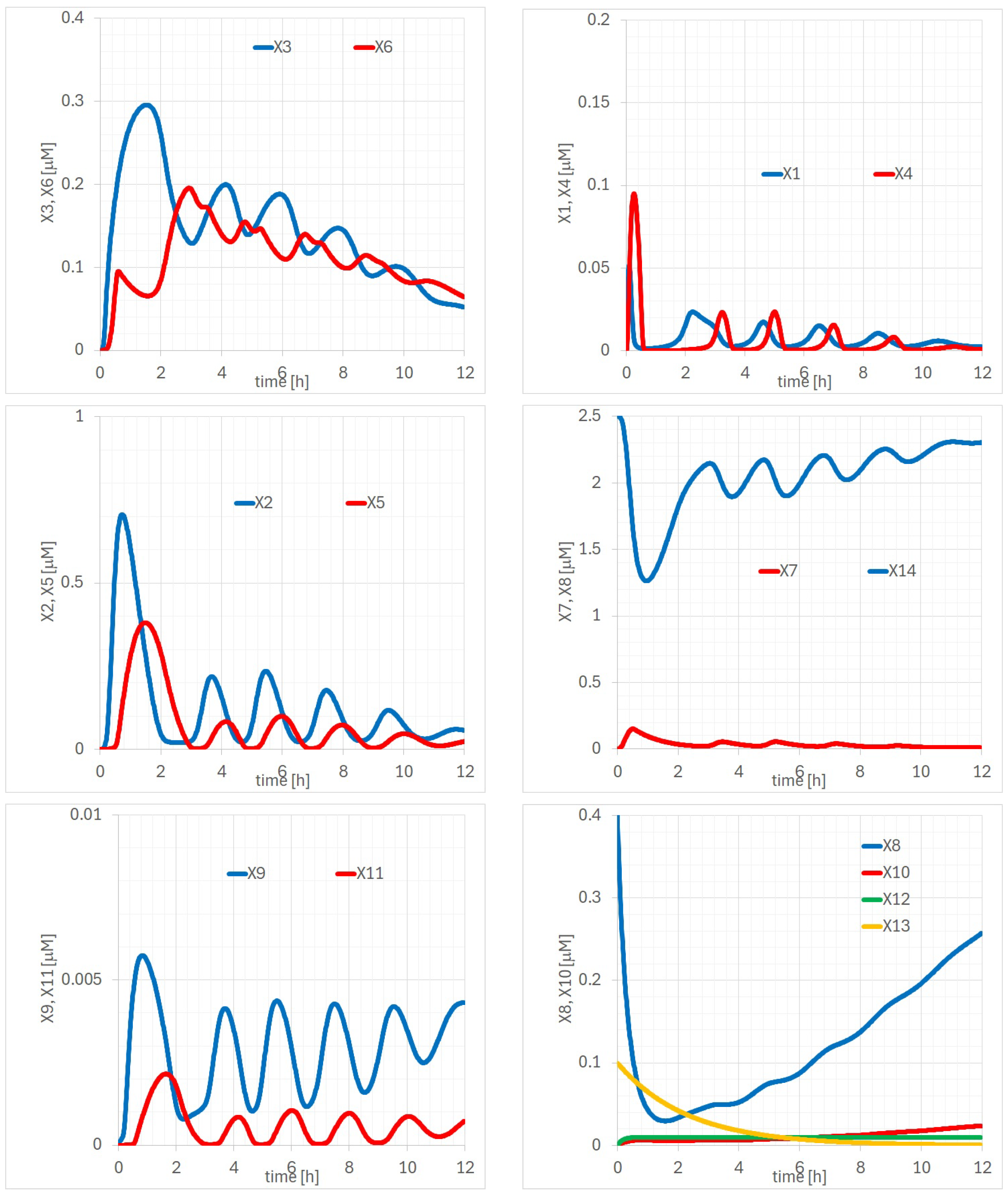
Appendix A. Detailed Analysis of Time Evolutions of RelBratio with the 14 Parameters

To investigate the effects of changes in parameters (1)–(14), we performed calculations of the time evolutions presented in Figure A1 for R e l B r a t i o with parameters of ( t o t a l R e l B , t o t a l I κ B α ) = (left) (4, 2.5), (center) (0.4, 2.5), and (right) (0.4, 25) [ μ M]; the legends 0 of the red lines denote the scenario where all parameters were configured to PAVs, and legends 1, 2, …, 14 indicate configurations where parameters s q , k a , …, d e g 2 were each assigned to EMVs, with all other elements set as PAVs. The differences in the time evolutions for parameters (1) s q , (3) t r a , (4) d e g 1 , (6) s p , (10) t r r 1 , (12) d r m , and (14) d e g 2 are distinctly shown by the thick lines in the upper section of Figure A1, clearly indicating significant deviations from the red medium line marked as (0). However, time evolutions in the lower section of Figure A1 for parameter configurations where any one of (2) k a , (5) k p , (7) u p , (8) s r , (9) u r , (11) d r , or (13) e r was set to its EMV did not exhibit significant deviations from the red medium line marked as (0).
Figure A1. Time evolutions of R e l B r a t i o with parameters of ( t o t a l R e l B , t o t a l I κ B α ) = (left) (4, 2.5), (center) (0.4, 2.5), and (right) (0.4, 25) [ μ M]. The legend 0 of the red line in Figure A1 represents the case where all parameters are set to the PAV, while (1)–(14) indicate cases where one of parameters (1)–(14) is set to the EMV. (Upper) time evolutions with the EMVs of parameters (1) s q , (3) t r a , (4) d e g 1 , (6) s p , (10) t r r 1 , (12) d r m , and (14) d e g 2 ; (lower) time evolutions with the EMVs of parameters (2) k a , (5) k p , (7) u p , (8) s r , (9) u r , (11) d r , and (13) e r .
Mca 29 00062 g0a1

Appendix B. Bifurcation Analysis

For bifurcation analysis, a simplified KO model (Figure 1) was used instead of the full model. Although the time evolution calculated with the KO model differed from that of the full model, it exhibited similar outcomes in terms of saturation, oscillation, and singular events, as depicted in the time evolutions presented in Figure A2.
Figure A2. Time evolutions of R e l B r a t i o for various ( t o t a l R e l B , t o t a l I κ B α ) of the p100KO-M with time ranges of (left) 0–10 and (right) 90–100 h.
Mca 29 00062 g0a2

Appendix B.1. Algorithm for Finding the Steady State

Equilibrium stability analysis is a method used to determine the stability around an equilibrium point via the evaluation of the eigenvalues of a matrix. Ordinary differential Equations (2a), (2b), (2d), (2e), (2f), and (2g) can be represented as a vector using the following equations:
(A1a) d d t X = f ( X ) , (A1b) X = ( X 1 , X 2 , X 4 , X 5 , X 6 , X 7 ) , (A1c) f = ( f 1 , f 2 , f 4 , f 5 , f 6 , f 7 ) , (A1d) f 1 ( X ) = s q X 1 + d e g 1 ( t o t a l R e l B X 1 X 4 X 6 ) k a X 1 X 2 , f 2 ( X ) = ( d 1 + s 1 ) X 2 + u 1 X 5 (A1e) + t r 1 X 7 ( t o t a l I κ B α t o t a l R e l B + X 1 X 2 + X 4 X 5 ) k a X 1 X 2 , (A1f) f 4 ( X ) = s q X 1 k a X 4 X 5 , (A1g) f 5 ( X ) = s 1 X 2 u 1 X 5 k a X 4 X 5 , (A1h) f 6 ( X ) = u a X 6 + k a X 4 X 5 , (A1i) f 7 ( X ) = t r a X 4 d 3 X 7 .
The equilibrium values ( X i * ) can be determined by extending these time evolutions to infinity for X i . The equilibrium point can be determined using the method of steepest decent [27,28] with a sequential bisection method [29].

Appendix B.2. Linearization and Eigenvalue Problems

By performing a Taylor expansion of f ( X ) near X X * , the following expression can be obtained.
f i ( X ) = f i ( X * ) + j = 1 2 , 4 , 5 , 6 , 7 ( X j X j * ) f i ( X ) X j X = X * + o [ ( X j X j * ) ( X k X k * ) ] , i , j , k = 1 , 2 , 4 , 5 , 6 , 7
If X is in the neighborhood of X * , we can approximate the expression by summing the terms up to the first order, ignoring terms of the second order and higher. When Equation (A1) has an equilibrium point, the stability of the fixed point is evaluated using eigenvalues of the Jacobian matrix. The linearized equation is expressed as follows.
(A3a) d d t x i = j = 1 2 , 4 , 5 , 6 , 7 f i ( X ) X j X = X * A i j x j , i = 1 , 2 , 4 , 5 , 6 , 7 ,
for x i = X i X i * ,
(A3b) A 11 = s q d e g 1 k a X 2 * , A 12 = k a X 1 * , A 14 = d e g 1 , A 16 = d e g 1 , A 21 = t r 1 X 7 * k a X 2 * , A 22 = d 1 s 1 t r 1 X 7 * k a X 1 * , A 24 = t r 1 X 7 * , A 25 = u 1 t r 1 X 7 * , (A3c) A 27 = t r 1 ( t o t a l I κ B α t o t a l R e l B + X 1 * X 2 * + X 4 * X 5 * ) , (A3d) A 41 = s q , A 44 = k a X 5 * , A 45 = k a X 4 * , (A3e) A 52 = s 1 , A 54 = k a X 5 * , A 55 = u 1 k a X 4 * , (A3f) A 64 = k a X 5 * , A 65 = k a X 4 * , A 66 = u a , (A3g) A 74 = t r a , A 77 = d 3 ,
where the fixed points ( X * ) are defined as points satisfying f ( X * ) = 0 . The Jacobian matrix ( A i j , i , j = 1 , 2 , 4 , 5 , 6 , 7 , ) in Equations ()–() has eigenvalues of λ . If the maximum of the real parts of the eigenvalues ( max [ ( λ ) ] ) is positive, an oscillation is observed. Consequently, the corresponding imaginary part of the eigenvalue ( ( λ ) ) becomes a value close to the angular oscillation frequency. Solving the eigenvalue problem of the Jacobian can reveal the following three states:
  • If all the eigenvalues of the Jacobian have negative real parts, then the equilibrium point ( X * ) is asymptotically stable.
  • If any eigenvalue of the Jacobian has a positive real part, then X * becomes unstable.
  • When complex eigenvalues appear in the Jacobian, X approaches X * while oscillating.
Figure A3 shows the bifurcation diagrams for t o t a l R e l B and t o t a l I κ B α in p100KO-M, where the orange lines correspond to max [ ( λ ) ] , i.e., the maximum real part of eigenvalues, and the blue lines represent ( λ ) , i.e., the imaginary part of the corresponding eigenvalues.
Figure A3. Bifurcation diagrams for t o t a l R e l B (A) and t o t a l I κ B α (B) in p100KO-M for the calibrated parameters. Dependencies of the t o t a l R e l B (A) and t o t a l I κ B α (B) are fixed at t o t a l I κ B α = 2.5 μ M and t o t a l R e l B = 0.4 μ M, respectively.
Mca 29 00062 g0a3
The numerical analysis of the bifurcation diagrams shown in Figure A3 revealed that the linearized matrix around the equilibrium point had complex eigenvalues with (1) zero ( λ ) in the range of t o t a l R e l B = 1.59–4.00 μ M and (2) nonzero ( λ ) in the range of t o t a l R e l B = 0.40–1.59 μ M with t o t a l I κ B α = 2.5 μ M, corresponding to the (1) saturation and (2) oscillation events, respectively. From the period of temporal evolutions shown in Figure A2, the period of the oscillation events was found to be 1.52, 1.87, 1.87, and 1.40 h for ( t o t a l R e l B , t o t a l I k B a ) = (0.8, 2.5), (0.4, 2.5), (0.4, 5.0), and (0.4, 12.5) [ μ M], respectively. These values were close to the values of 1.77, 3.32, 3.66, and 1.65 h calculated from the eigenvalues in Table A1. In the oscillation events, the periods of temporal evolutions indicated approximate agreement with the periods converted from each angular frequency considered as imaginary parts of the eigenvalues. However, discrepancies in these periods were considered to be caused by errors in the eigenvalue calculations.
Table A1. Equivalent periods calculated from ( λ ) s for each ( t o t a l R e l B , t o t a l I κ B α ).
totalRelB [ μ M]totalIkBa [ μ M] ( λ ) [rad/min]Equivalent Period: 2 π / ( λ ) [h]
0.82.50.05901.77
0.42.50.03163.32
0.45.00.02863.66
0.412.50.06361.65
Figure A4 shows the dependencies of R e l B r a t i o on t o t a l R e l B and t o t a l I κ B α , calculated based on the bifurcation diagrams presented in Figure A3. R e l B r a t i o was found to be 0.546, 0.271, 0.342, 0.412, 0.395, 0.334, and 0.301 for ( t o t a l R e l B , t o t a l I k B a ) = (4, 2.5), (2, 2.5), (0.8, 2.5), (0.4, 2.5), (0.4, 5), (0.4, 12.5), and (0.4, 25) [ μ M], respectively. These values coincided with the equilibrium values of the time evolutions in Figure A2, suggesting the accurate modeling of the system’s behavior under various conditions.
Figure A4. R e l B r a t i o —(left) t o t a l R e l B and (right) t o t a l I κ B α dependencies of p100KO-M for the calibrated parameters. The dependencies of the t o t a l R e l B and t o t a l I κ B α are fixed at t o t a l I κ B α = 2.5 μ M and t o t a l R e l B = 0.4 μ M, respectively.
Mca 29 00062 g0a4
Figure A5 presents the dependencies of the loss function (L = f ( X * ) 2 ) on t o t a l R e l B and t o t a l I κ B α , as derived from the bifurcation diagrams presented in Figure A3. These dependencies indicated two abrupt changes in the loss function—at t o t a l R e l B ≅ 1.3 μ M for t o t a l κ B α = 2.5 μ M and at t o t a l κ B α ≅ 15 μ M for t o t a l R e l B = 0.4 μ M. These points signified state transitions from a stable state with L 10 24 to an unstable state with 10 9 L 10 3 . This indicated that these two points mark transitions from oscillatory events to saturation and singular events, respectively. The temporal evolutions depicted in Figure A2 show the oscillation events at t o t a l κ B α = 2.5 μ M for t o t a l R e l B = 0.8, 0.4 μ M and at t o t a l R e l B = 0.4 μ M for t o t a l κ B α = 5, 12.5 μ M. These points ( t o t a l R e l B , t o t a l κ B α ) were within the range of oscillatory events described in the bifurcation analysis. This demonstrated the model’s reasonable accuracy in capturing the dynamics of the system.
Figure A5. Loss function—(left) t o t a l R e l B and (right) t o t a l I κ B α dependencies of p100KO-M for the calibrated parameters. The dependencies of the t o t a l R e l B and t o t a l I κ B α are fixed at t o t a l I κ B α = 2.5 μ M and t o t a l R e l B = 0.4 μ M, respectively.
Mca 29 00062 g0a5

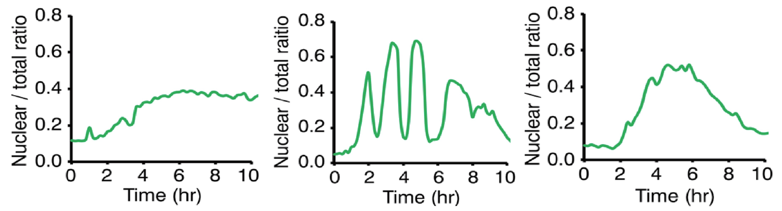
Appendix C. Experimental Methods and Data Details

Figure 3 illustrates the time evolutions of RelB nuclear translocation. The experiment involved the following steps:
  • Cell preparation: MEF (mouse embryonic fibroblast) cells stably expressing RelB-Venus were used. These cells were modified with a retroviral vector in which the nuclear localization signal (NLS) from the nuclear fluorescent protein EYFP-Nuc was fused to the 3’ end of mCherry [20].
  • Antibody treatment: Cells were treated with 0.3 μ g/mL anti-LT β R antibody to induce RelB nuclear translocation. This treatment activates the non-canonical NF- κ B pathway [20].
  • Time-lapse imaging: Cells were observed using time-lapse imaging, and the fluorescence intensity in the nucleus and the entire cell was measured. These data show the nuclear fluorescence intensity of RelB, particularly the time evolution following stimulation with 0.3 μ g/mL anti-LT β R antibody. The experiment observed patterns of RelB nuclear translocation and oscillation after stimulation [20].

Appendix C.1. Empirical Evidence for the Non-Canonical NF-κB Pathway

The oscillation and nuclear translocation of RelB provide crucial evidence for the involvement of the non-canonical NF- κ B pathway. In this pathway, p100 processing generates p52, which translocates to the nucleus, along with RelB. This process is critical for functions such as B-cell maturation, bone metabolism, and lymphoid organ formation [20]. Specifically, this study highlights that the oscillation of RelB is essential for controlling transcriptional activity [20]. These findings provide new insights into how the non-canonical NF- κ B pathway functions in immune responses and cellular responses.

References

  1. Cheong, R.; Hoffmann, A.; Levchenko, A. Understanding NF-κB signaling via mathematical modeling. Mol. Syst. Biol. 2008, 4, 192. [Google Scholar] [CrossRef] [PubMed]
  2. Basak, S.; Behar, M.; Hoffmann, A. Lessons from mathematically modeling the NF-κB pathway. Immunol. Rev. 2012, 246, 221–238. [Google Scholar] [CrossRef] [PubMed]
  3. Shih, V.F.-S.; Tsui, R.; Caldwell, A.; Hoffmann, A. A single NFκB system for both canonical and non-canonical signaling. Cell Res. 2011, 21, 86–102. [Google Scholar] [CrossRef] [PubMed]
  4. Pomerantz, J.-L.; Baltimore, D. Two pathways to NF-κB. Mol. Cell 2002, 10, 693–695. [Google Scholar] [CrossRef]
  5. Oeckinghaus, A.; Ghosh, S. The NF-κB family of transcription factors and its regulation. Cold Spring Harb. Perspect. Biol. 2009, 1, a000034. [Google Scholar] [CrossRef] [PubMed]
  6. Hayden, M.S.; Ghosh, S. Shared principles in NF-κB signaling. Cell 2008, 132, 344–362. [Google Scholar] [CrossRef] [PubMed]
  7. Basak, S.; Shih, V.F.-S.; Hoffmann, A. Generation and activation of multiple dimeric transcription factors within the NF-κB signaling system. Mol. Cell. Biol. 2008, 28, 3139–3150. [Google Scholar] [CrossRef] [PubMed]
  8. Hoffmann, A.; Natoli, G.; Ghosh, S. Transcriptional regulation via the NF-κB signaling module. Oncogene 2006, 25, 6706–6716. [Google Scholar] [CrossRef]
  9. Mitchell, S.; Vargas, J.; Hoffmann, A. Signaling via the NFκB system. WIREs Syst. Biol. Med. 2016, 8, 227–241. [Google Scholar] [CrossRef] [PubMed]
  10. Iwai, K. Diverse ubiquitin signaling in NF-κB activation. Trends Cell Biol. 2012, 22, 355–364. [Google Scholar] [CrossRef] [PubMed]
  11. Vallabhapurapu, S.; Matsuzawa, A.; Zhang, W.; Tseng, P.-H.; Keats, J.J.; Wang, H.; Vignali, D.A.; Bergsagel, P.L.; Karin, M. Nonredundant and complementary functions of TRAF2 and TRAF3 in a ubiquitination cascade that activates NIKdependent alternative NF-κB signaling. Nat. Immunol. 2008, 9, 1364. [Google Scholar] [CrossRef] [PubMed]
  12. Xiao, G.; Harhaj, E.W.; Sun, S.-C. NF-κB-inducing kinase regulates the processing of NF-κB2 p100. Mol. Cell 2001, 7, 401–409. [Google Scholar] [CrossRef] [PubMed]
  13. Nelson, D.E.; Ihekwaba, A.E.C.; Elliott, M.; Johnson, J.R.; Gibney, C.A.; Foreman, B.E.; Nelson, G.; See, V.; Horton, C.A.; Spiller, D.G.; et al. Oscillations in NF-κB Signaling Control the Dynamics of Gene Expression. Science 2004, 306, 704–709. [Google Scholar] [CrossRef] [PubMed]
  14. Ashall, L.; Horton, C.A.; Nelson, D.E.; Paszek, P.; Harper, C.V.; Sillitoe, K.; Ryan, S.; Spiller, D.G.; Unitt, J.F.; Broomhead, D.S.; et al. Pulsatile Stimulation Determines Timing and Specificity of NF-κB–Dependent Transcription. Science 2009, 324, 242–247. [Google Scholar] [CrossRef] [PubMed]
  15. Hatanaka, N.; Seki, T.; Inoue, J.; Tero, A.; Suzuki, T. Critical roles of IκBα and RelA phosphorylation in transitional oscillation in NF-κB signaling module. J. Theor. Biol. 2019, 462, 479–489. [Google Scholar] [CrossRef] [PubMed]
  16. Hoffmann, A.; Leung, T.H.; Baltimore, D. Genetic analysis of NF-κB/Rel transcription factors defines functional specificities. EMBO J. 2003, 22, 5530–5539. [Google Scholar] [CrossRef] [PubMed]
  17. Aggarwal, B.B. Signalling pathways of the TNF superfamily: A double-edged sword. Nat. Rev. Immunol. 2003, 9, 745–756. [Google Scholar] [CrossRef] [PubMed]
  18. Sun, S.-C. Non-canonical NF-κB signaling pathway. Cell Res. 2011, 21, 71–85. [Google Scholar] [CrossRef] [PubMed]
  19. Seki, T.; Yamamoto, M.; Taguchi, Y.; Miyauchi, M.; Akiyama, N.; Yamaguchi, N.; Gohda, J.; Akiyama, T.; Inoue, J. Visualization of RelB expression and activation at the single-cell level during dendritic cell maturation in Relb-Venus knock-in mice. J. Biochem. 2015, 158, 485–495. [Google Scholar]
  20. Seki, T. Analysis of Spatiotemporal Control Mechanism of Transcription Factor NF-κB. Ph.D. Thesis, Tokyo University, Tokyo, Japan, 2015. [Google Scholar]
  21. Lee, D.; Jayaraman, A.; Kwon, J. Identification of cell-to-cell heterogeneity through systems engineering approaches. AIChE J. 2020, 66, e16925. [Google Scholar] [CrossRef]
  22. Lee, D.; Jayaraman, A.; Kwon, J. Development of a hybrid model for a partially known intracellular signaling pathway through correction term estimation and neural network modeling. PLOS Comp. Biol. 2020, 16, e1008472. [Google Scholar] [CrossRef] [PubMed]
  23. Shih, V.F.-S.; Davis-Turak, J.; Macal, M.; Huang, J.Q.; Ponomarenko, J. Control of RelB during dendritic cell activation integrates canonical and noncanonical NF-κB pathways. Nat. Immunol. 2012, 13, 1162–1172. [Google Scholar] [CrossRef] [PubMed]
  24. Banoth, B.; Chatterjee, B.; Vijayaragavan, B.; Prasad, M.V.R.; Roy, P.; Basak, S. Stimulus-selective crosstalk via the NF-κB signaling system reinforces innate immune response to alleviate gut infection. eLife 2015, 4, e05648. [Google Scholar] [CrossRef] [PubMed]
  25. Dobrzanski, P.; Ryseck, R.; Bravo, R. Differential interactions of Rel -NF-κB complexes with IκBα determine pools of constitutive and inducible NF-κB activity. EMBO J. 1994, 13, 4608–4616. [Google Scholar] [CrossRef] [PubMed]
  26. Almaden, V.; Tsui, R.; Liu, Y.C.; Birnbaum, H.; Shokhirev, M.N.; Ngo, K.A.; Davis-Turak, J.C.; Otero, D.; Basak, S.; Rickert, R.C.; et al. A Pathway Switch Directs BAFF Signaling to Distinct NFκB Transcription Factors in Maturing and Proliferating B Cells. Cell Rep. 2014, 9, 2098–2111. [Google Scholar] [CrossRef] [PubMed]
  27. Lewis, J.; Lakshmivarahan, S.; Dhall, S. Dynamic Data Assimilation: A Least Squares Approach; Cambridge University Press: Cambridge, UK, 2006. [Google Scholar]
  28. Meza, J. Steepest Descent; Technical Report in Lawrence Berkeley National Lab; Lawrence Berkeley National Laboratory: Berkeley, CA, USA, 2010. [Google Scholar]
  29. Vanderplaats, G.N. Numerical Optimization Techniques for Engineering Design: With Applications, 3rd ed.; Vanderplaats Research and Development, Inc.: Colorado Springs, CO, USA, 2001. [Google Scholar]
Figure 1. Model diagram and a simulation result of p100KO-M. (A) Model diagram based on experimental data and one assumption. A feedback loop from p50/RelB to I κ B α is required to obtain the self-sustained oscillation of RelB. (B) Simulation result of p100KO-M. The equilibrium points of p100KO-M are unstable, and the self-sustained oscillation of RelB is caused by a stable limit cycle.
Mca 29 00062 g001
Figure 2. NC-FM model diagram. (A) Full pathway models of the NF- κ B non-canonical pathway extended from p100KO-M. (B) Time evolutions of R e l B r a t i o with parameters of ( t o t a l R e l B , t o t a l I κ B α ) = (left) (4, 2.5), (center) (0.4, 2.5), and (right) (0.4, 25) [ μ M]. Three events, namely saturation, oscillation, and single events, were reproduced by sensitivity analysis, changing t o t a l R e l B and t o t a l I κ B α in NC-FM.
Mca 29 00062 g002
Figure 3. Experimental results of time evolutions of RelB nuclear translocation [20], which show three types of dynamics, namely (left) nuclear retention (saturation), (center) oscillation, and (right) single events.
Mca 29 00062 g003
Figure 4. Time evolutions of R e l B r a t i o with values of ( t o t a l R e l B , t o t a l I κ B α ) = (left) (4, 2.5), (center) (0.4, 2.5), and (right) (0.4, 25) [ μ M]. The three legends mean that e r is set to 10 3 , 1.9 × 10 7 , and 3 × 10 8 [ μ M/min].
Mca 29 00062 g004
Figure 5. Time evolutions of R e l B r a t i o with parameters of ( t o t a l R e l B , t o t a l I κ B α ) = (left) (4, 2.5), (center) (0.4, 2.5), and (right) (0.4, 25) [ μ M]. Legend 0 of the red line represents the case where all parameters are set to the PAV, while legends 1, 3, 4, 6, 10, 12, and 14 indicate cases where one of the parameters ( s q , t r a , d e g 1 , s p , t r r 1 , d r m , or d e g 2 ) is set to the EMV.
Mca 29 00062 g005
Figure 6. Time evolutions of X i , i = 1 , 8 of the p100KO model: (upper left) ( X 3 , X 6 ), (right-upper) ( X 1 , X 4 ), (lower left) ( X 2 , X 5 ), and (lower right) ( X 2 , X 5 ) [ μ M].
Mca 29 00062 g006
Figure 7. Time evolutions of X i , i = 1 , 14 of the NC-FM; (left-upper) ( X 3 , X 6 ), (right-upper) ( X 1 , X 4 ), (left-middle) ( X 2 , X 5 ), (right-middle) ( X 7 , X 14 ), (left-lower) ( X 9 , X 11 ), (right-lower) ( X 8 , X 10 , X 12 , X 13 ) [ μ M], respectively.
Mca 29 00062 g007
Table 1. Correspondence table between variables and molecules of non-canonical pathway models.
ValueMolecule p100KO-MNC-FM
X 1 p52/RelBp52/RelB
X 2 I κ B α I κ B α
X 3 I κ B α /p52/RelBI κ B α /p52/RelB
X 4 p52/RelBip52/RelBi
X 5 I κ B α i I κ B α i
X 6 I κ B α /p52/RelBiI κ B α /p52/RelBi
X 7 unknownunknown
X 8 inactive I κ B α p100/RelB
X 9 -p100
X 10 -p100/RelBi
X 11 -p100i
X 12 -p100 mRNA
X 13 -active IKK
X 14 -inactive I κ B α
Table 2. Reactions of RelB and I κ B α in the non-canonical pathway.
PathwayDescription
(i)p50/RelB → p50/RelBiCytoplasmic p50/RelB moves into the nucleus
(ii)I κ B α I κ B α i I κ B α shuttles between the nucleus and cytoplasm
(iii)p50/RelB/I κ B α i → p50/RelB/I κ B α Nuclear p50/RelB exports to the cytoplasm by binding to I κ B α
(iv)p50/RelB/I κ B α → p50/RelBI κ B α of p50/RelB/I κ B α degrades in the cytoplasm
Table 3. Parameters of partially numerically adjusted values (PAVs).
SymbolValueUnitDescription
s q 0.2 *1/minp52/RelB nuclear import
k a 30 *1/ μ M minp52/RelB association
d 1 0.00678 1/minI κ B α degradation
s 1 0.018 1/minI κ B α nuclear import
t r 1 0.2448 1/ μ M minI κ B α activation
u 1 0.012 1/minI κ B α nuclear export
t r a 0.1 * μ M/minp52/RelB-dependent (unknown factor) transcription
d 3 0.0168 1/minI κ B α mRNA degradation
u a 0.012 *1/minI κ B α /p52/RelB nuclear export
d e g 1 0.1 *1/minI κ B α of I κ B α /NF- κ B dissociation
k p 50 *1/ μ M minp52/RelB replacement with p100/RelB
s p 0.001 *1/minp100/RelB nuclear import
u p 0.01 *1/minp100/RelB nuclear export
s r 0.01 *1/minp100 nuclear import
u r 0.01 *1/minp100 nuclear export
t r r 1 0.1 *1/minp100 protein translation
d r 0.1 *1/minp100 degradation
d r m 0.1 *1/minp100 mRNA degradation
e r 0.001 * μ M/minp100 mRNA transcription
d e g 2 0.5 *1/ μ M minp100 processing
d 2 0.0072 1/minIKK degradation
t o t a l R e l B 0.4 * μ MTotal amount of RelB in a cell in the oscillation event
t o t a l I κ B α 2.5 * μ MTotal amount of I κ B α in a cell in the oscillation event
a c t i v e I K K 0.1 * μ MTotal amount of activeIKK in a cell
Nelson et al. [13]. * Data fittings.
Table 4. Summary of PAVs and EMVs, where PAVs are same as in Table 3.
SymbolPAVEMVUnitDescription
s q 0.2 *5.4 1/minp52/RelB nuclear import
k a 30 *51 1/ μ M minp52/RelB association
d 1 0.00678 as left1/minI κ B α degradation
s 1 0.018 as left1/minI κ B α nuclear import
t r 1 0.2448 as left1/ μ M minI κ B α activation
u 1 0.012 as left1/minI κ B α nuclear export
t r a 0.1 *0.01 * μ M/minp52/RelB-dependent (unknown factor) transcription
d 3 0.0168 as left1/minI κ B α mRNA degradation
u a 0.012 *as left1/minI κ B α /p52/RelB nuclear export
d e g 1 0.1 *0.032 1/minI κ B α of I κ B α /NF- κ B dissociation
k p 50 *0.13 1/ μ M minp52/RelB replacement with p100/RelB
s p 0.001 *0.028 1/minp100/RelB nuclear import
u p 0.01 *0.42 1/minp100/RelB nuclear export
s r 0.01 *0.045 1/minp100 nuclear import
u r 0.01 *0.012 1/minp100 nuclear export
t r r 1 0.1 *0.5 #1/minp100 protein translation
d r 0.1 *0.4 #1/minp100 degradation
d r m 0.1 *1.6 × 10 3  #1/minp100 mRNA degradation
e r 0.001 *1.9 × 10 7  # μ M/minp100 mRNA transcription
d e g 2 0.5 *4.2 #1/ μ M minp100 processing
d 2 0.0072 as left1/minIKK degradation
t o t a l R e l B 0.4 *0.08 $ μ MTotal amount of RelB in a cell in the oscillation event
t o t a l I κ B α 2.5 *0.6 * μ MTotal amount of I κ B α in a cell in the oscillation event
a c t i v e I K K 0.1 *as left μ MTotal amount of activeIKK in a cell
Shih et al. [23]. Nelson et al. [13]. * Data fittings. # Banoth et al. [24]. $ Ashall et al. [14].
Disclaimer/Publisher’s Note: The statements, opinions and data contained in all publications are solely those of the individual author(s) and contributor(s) and not of MDPI and/or the editor(s). MDPI and/or the editor(s) disclaim responsibility for any injury to people or property resulting from any ideas, methods, instructions or products referred to in the content.

